Tool orchestration for modeling, verification and analysis of collaborating autonomous machines

(1)

V¨

aster˚

as, Sweden

Thesis for the Degree of Master of Science (60 credits) in Computer

Science with Specialization in Software Engineering

TOOL ORCHESTRATION FOR MODELING,

VERIFICATION AND ANALYSIS OF

COLLABORATING AUTONOMOUS

MACHINES

Pavle Mrvaljevi´c

pmc19001@student.mdh.se

Examiner: Antonio Cicchetti

M¨

alardalen University, V¨

aster˚

as, Sweden

Supervisors: Marjan Sirjani and Anas Fattouh

M¨

alardalen University, V¨

aster˚

as, Sweden

Company supervisor: Stephan Baumgart

Volvo CE, Eskilstuna

(2)

Abstract

System of systems (SoS) is a collective of multiple system units that have a common purpose. In this thesis, the Volvo Electric Site is investigated as an example case study in which safety and performance properties of collaborating autonomous machines are evaluated and analyzed. For-mal methods in software engineering aim to prove the correctness of the system by evaluating its mathematical model. We use an actor-based framework, AdaptiveFlow, for modeling system func-tionalities and timing features. The aim is to link an abstract model evaluation and a simulation of real-world cases that are deployed in the VCE Simulator. In addition, it is necessary to make sure that AdaptiveFlow provides correct-by-design scenarios. The verification is conducted by de-veloping an orchestration method between the AdaptiveFlow framework and the VCE Simulator. A tool named VMap is developed throughout this thesis for automated mapping of the input models of AdaptiveFlow and the VCE Simulator to make the orchestration possible. Furthermore, Adap-tiveFlow is perceived in two different ways, as a design tool, and as an analysis tool. The models created in AdaptiveFlow are directly mapped to the VCE Simulator by using the VMap tool where the VCE Simulator is used as a testbed for checking these models. The outcome of this thesis is re-flected in the establishment of a mapping pattern between AdaptiveFlow inputs and VCE simulator by developing the VMap tool for automatic mapping. It was shown that there is a natural mapping between the AdaptiveFlow models and VCE simulator inputs. By using VMap, we can quickly get to the desired scenarios. Through the development of three different cases, the results show that it is possible to design safe and optimal scenarios by orchestrating the AdaptiveFlow and the VCE Simulator using the VMap tool as well as the correlation between results from AdaptiveFlow and VCE Simulator.

(3)

List of Figures

1 Automated Hauler . . . 2

2 Volvo Electric Site . . . 2

3 AGV system properties . . . 9

4 Research Method . . . 12

5 AdaptiveFlow workflow [1] . . . 14

6 AdaptiveFlow environment [1] . . . 15

7 Tools used with their inputs and outputs . . . 17

8 Conversion from AdaptiveFlow inputs to VCE guideline file . . . 18

9 Scenario developed by following the guideline . . . 19

10 Mapping segment attributes to simulator elements . . . 21

11 Mapping PoI attributes to simulator Edge attributes . . . 22

12 Machine safety zone . . . 23

13 Fleet management scenario - Control System . . . 25

14 Loading site logic . . . 25

15 AdaptiveFlow environment of initial scenario . . . 27

16 Fleet Management: Path index and autonomous hauler speed . . . 32

17 Fleet Management: Traveled distance of each autonomous hauler . . . 32

18 Fleet Management: Operating time in AdaptiveFlow and VCE Simulator . . . 32

19 Volvo Electric Site Schema . . . 33

20 Volvo Electric Site: Model design . . . 34

21 Volvo Electric Site: Transformation from guideline to the Simulator environment . 35 22 Volvo Electric Site: Path index and autonomous hauler speed . . . 36

23 Volvo Electric Site: Traveled distance of each autonomous hauler . . . 36

24 Volvo Electric Site: Operating time in AdaptiveFlow and VCE Simulator . . . 36

25 Counter-example: Model design . . . 37

26 Counter-example: Scenario execution . . . 38

27 Counter-example: Simulator environment . . . 39

28 Counter-example: The path played by each autonomous hauler . . . 40

29 Counter-example: Path index and autonomous hauler speed . . . 40

30 Counter-example: Traveled distance of each autonomous hauler . . . 40

(6)

1. Introduction

Collaborative systems, commonly referred to as system-of-systems (SoS), represent a collective of independent systems that cooperate to achieve a common goal [1]. Each unit of the SoS is task-oriented and these tasks are executed in the collaboration with other units. Taking into account the complexity of the SoS we should use a suitable verification method which would ensure that the system matches the desired design specification. In order to design such systems, the techniques for the analysis should be defined. The most common techniques used are testing, simulation, assertion check, lightweight formal verification, and statistical model checking. Considering the complexity of collaborative systems, designing models for different levels of abstraction would prove helpful. As there are many unpredictable factors in this system it is desirable to build adaptive models that would be able to respond to these obstacles. Due to the fact that modern machines have embedded software, it is possible to create a collaborative system that would automatize the workflow. For this thesis, it is envisioned to conduct modeling and analysis of collaborating autonomous heavy machines for the Volvo construction site in order to check their safety and performance properties. In order for the appropriate model to evolve, it is necessary to consider all the characteristics of the system. The main focus is on the modeling of the fleet control system for the scenario developed for the VCE Simulator. The simulator provides a convenient representation of real-world cases through which the performance and safety would be evaluated.

There are various modeling languages and techniques available with different characteristics and supporting tools. Since the nature of this system is distributed and concurrent we should use appropriate tools for modeling and analysis. The suitable paradigm which would address this is the usage of actor models introduced by Hewitt [2]. This actor model has been later developed as an object-based functional language by Agha [3]. In this case, Rebeca modeling language is used due to the fact that it targets distributed and concurrent systems and its capability to execute assertion checks and deadline misses. Rebeca (Reactive Objects Language) is an open-source actor-based modeling language with a formal foundation that has a purpose to bridge a gap between software engineers and formal method community [4]. It has a syntax similar to Java and it is a platform for developing object-based concurrent systems that are supported by a model checking toolset [1]. Additionally, Rebeca has a feature to model timing constraints by using its real-time extension, Timed Rebeca [5]. Modeling and analyzing this collaborative system is executed with the AdaptiveFlow framework. This framework is based on the Eulerian model and it makes modeling and analyzing track-based flow management systems possible [6]. In order to verify safety and performance properties, the VCE simulator is seen as a testbed.

To conduct this experiment first it is necessary to build TRebeca models with the AdaptiveFlow framework. In this framework, tracks are modeled as actors and moving objects (autonomous machines) as messages [6]. Next, the checking of performance and safety properties needs to be executed. Safety and progress properties include the minimum distance between the machines, relation between the speed of a machine and its distance from others, and deadlock checks. The performance properties comprise the system throughput of several collaborating machines and the least waiting time for a service request to be completed. It is important to adjust mentioned properties with what VCE simulator can provide. The third step is to map specified properties to the VCE simulator and verify if the properties hold. Finally, the mapping between AdaptiveFlow inputs and VCE simulator inputs needs to be automatized.

In this work, we propose a tool orchestration method in which we use both AdaptiveFlow and VCE Simulator as a complete tool stack for verification and evaluation of collaborating autonomous haulers. To retrieve results and to provide a depth of this research, we conducted experiments on three different cases. Each case takes a different approach to tool orchestration to demonstrate the variety of methods of applying these tools.

The main goal is to close the loop in model-driven development in which the usability of Adap-tiveFlow is shown. The 2D model abstraction is lowered to a more realistic representation of the system in order to see whether there is a correlation in results. The mappable attributes/elements are recognized by which the mapping procedure has been developed. The main challenges and limitations have also been represented.

(7)

1.1. Problem Formulation

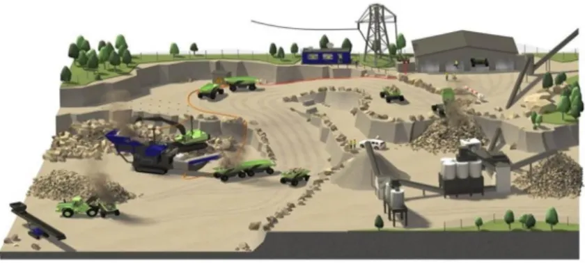
In this project, the case study of the electrified site project by Volvo Construction Equipment is considered. This case is based on collaborating autonomous machines, referred to as automated haulers, shown in Figure 1, which purpose is to perform several tasks such as loading, unloading, charging and material transport by operating in the fleet manner [7]. Autonomous machines have a centralized fleet control server that sends information to the machines in a certain time interval.

Figure 1: Automated Hauler

In this case, AdaptiveFlow is perceived as both, design and analysis tool for collaborative systems which generates TRebeca models. On the other hand, VCE Simulator acts as a testing environment for modeled systems. The scope of this thesis includes several objectives. The first step is to analyze the VCE Simulator by developing a suitable TRebeca model of the quarry site scenario similar to the one on Figure 2 with machine operations and conduct safety and performance checks. For this part, it is necessary to design an adequate environment in which the spots for points of interest (PoIs), as well as available segments of the environment, would be defined. This is done with the AdaptiveFlow framework. Furthermore, the configuration of the whole system should be specified. Based on the TRebeca model generated from defined specifications, it is required to perform a verification of that model. If the verification proves to be successful, the next step is to investigate how to perform a mapping between AdaptiveFlow inputs and VCE simulator. Based on this we will run the simulator and see whether the mapping was successful. The final phase is to discover how to automatize this mapping process.

(8)

1.2. Research Questions

The general question is if AdaptiveFlow framework (the design and analysis methods) is effective for model-based development of fleet management systems. This framework operate at an abstract level and to examine its effectiveness we need to see if the analysis results are valid during the simulation when we add more concrete and detailed features. This question can be broken down into the following research questions.

• RQ1: How usable is the design model of AdaptiveFlow for model-based devel-opment of fleet management systems?

The difference in the level of abstraction in the two tools introduces limitations and challenges. To examine the usability we need to check how challenging it is to map TRebeca models to more concrete models in the VCE simulator. Considering the implementation within the VCE Simulator and the nature of AdaptiveFlow, it is necessary to come up with an answer to what the limitations are when it comes to mapping. To answer this question, on one hand, we must take into account the complexity of the environment in the VCE Simulator, which is actually a depiction of the real system in 3D. On the other hand, the system in AdaptiveFlow is represented as a 2D abstraction. We have to find a common ground between the two in order to carry out appropriate mapping. Taking this into account, we can concretize the main question into following sub-questions:

– What is the mapping pattern between AdaptiveFlow inputs and VCE Simulator inputs? – What are the major challenges and limitations in building this automated mapping? • RQ2: How much the safety and performance properties verified by AdaptiveFlow

are valid for cooperative construction machines in the VCE Simulator?

Since the AdaptiveFlow framework provides, with the design of TRebeca models, their ver-ification and performance evaluation, it is necessary to find a way to analyze these prop-erties inside the VCE Simulator. To answer this question, it is also necessary to perform an implementation within the VCE simulator that matches the inputs and logic defined in AdaptiveFlow. This question can be divided into sub-questions below.

– Are the design analysis results of AdaptiveFlow precise enough to be relied on and to be used for model-based development?

– How effective and precise can the results of analysis performed by AdaptiveFlow be?

1.3. Research Contributions

The contributions of the thesis that are the result of solving the problems described in Section 1.1. are listed below:

• Patterns for mapping inputs from AdaptiveFlow to VCE Simulator

In order to develop a mapping procedure, we extract mappable elements from the Adaptive-Flow inputs to VCE Simulator. These elements were identified through the reverse engineer-ing process in Section 6.1. The main problem is to find out how to transform a concept of the 2D environment of AdaptiveFlow to a complex 3D simulation scenario.

• The VMap tool developed for automating the mapping procedure

One of the aims of this thesis is not only to derive an algorithm that could be implemented for the mapping procedure but to also provide a proof of concept by developing a suitable tool. The major applicative contribution of this thesis work is the VMap tool that represents a link between an abstract representation of a collaborative system from AdaptiveFlow and a simulation that provides a representation of real-world cases. This tool could be viewed as a piece of the puzzle for the verification of collaborative systems in which multiple tools and frameworks are used. It uses AdaptiveFlow inputs as well as complementary information from the VCE Simulator input file (dynamic.content) to generate a 2D representation of VCE elements, such as vertices and edges, and a dynamic.content example file.

(9)

• Methods for evaluating collaborative system features through model verification and simulation

In this thesis, we have also dealt with the verification and evaluation of systems of the autonomous machines. This is done through orchestration of the AdaptiveFlow and the VCE Simulator. More explicitly, it is conducted by extracting the safety and performance results from the TRebeca models as well as from the simulation. The main problem is to find performance properties that can be measured in AdaptiveFlow as well as in the Simulator. The comparison of identified performance results is made on the basis of which the conclusions are drawn.

(10)

2. Background

To be able to understand the research contributions of this work, in this section a few crucial areas have been described. In this thesis, we have touched on topics such as actor-based modeling, system-of-systems, Automated Guided Vehicles (AGVs), formal verification and the tools which are used in order to realize this research. Rebeca modeling language will be explained in depth. In addition to that, we will go through the tools necessary to perform a model verification.

2.1. Model-Driven Development

Model-Driven Development (MDD), also referred to as Model-Driven Engineering (MDE), is a field in software engineering which has an aim to an abstract software system, simplify the development process and lower the cost of the implementation. The model in MDD is a representation of the system, including its structure and functionalities. Due to its simplicity, it is a good link in communication between engineers and clients. Thomas et al. [8] have derived the goals of MDD and some of them are listed below.

• Increase of development speed - This is achieved due to the automation of generating code

from defined models. Through one or more steps of transformation, this automation is

achieved.

• Enhancement of software quality - Through previously mentioned steps of transformation and usage of formal languages, the software quality will be enhanced since the modules from the software architecture will reappear in the implementation.

• Higher level of reusability - As properties such as system architecture, modeling language and transformation have been specified, they could be used as a foundation for other similar projects which increases the level of reusability.

• Manageability of complexity through abstraction - Often, there is an increase in system complexity, so it is necessary to simplify the representation of the system, which MDD does through abstracting system components and structure.

In this work, MDD was performed as we have created models of the concurrent, distributed system of autonomous machines by using the Rebeca modeling language which has been described in the upcoming sections.

2.2. Formal Methods

In software engineering, formal methods represent a set of techniques for development, verification and analysis of software systems. These techniques allow a more reliable design of complex systems by introducing a more mathematically-oriented approach to software development. Due to the discontinuous nature of software systems, minor changes could cause huge and unpredictable errors which highlight the difference in software engineering from other engineering disciplines [9]. This is why formal methods are essential for developing a robust and correctly designed system. When developing autonomous systems, such as the one covered in this thesis, the specification is arguably the biggest bottleneck in performing the verification and validation [10].

Even though formal methods do not guarantee the development of systems that are prone to errors, they do help in developing a greater understanding of the system, by pointing out the inconsistencies in system design. These flaws are of great importance due to the consequences that they could cause [11]. In our case, we are modeling a system that manages autonomous machines. In this field, suitable formal methods are imperative since they would decrease the cost of development of these systems to a great extent.

Formal methods can be categorized in several different ways. In [12] formal methods have been differentiated as lightweight vs. heavyweight and the application of formal methodologies has been defined horizontal and vertical. By the lightweight formal methods we refer to partial specification and do not require high expertise, which is in contrast to the heavyweight formal methods. The horizontal application of formal methods implies a formally designed software, whereas the vertical application is pointed to a correct-by-construction approach.

(11)

2.2.1. Formal specification

In systems development, formal specification is a set of techniques used for a better understanding and safer construction of systems based on mathematical representation [13]. These techniques are used to lower the cost of system construction and to prevent faults that would be more difficult and expensive to correct in further stages of development. In formal verification, multiple aspects of the system are covered. It can be used for multiple purposes such as better grasp of the system functionalities, analysis of properties of interest and directing the development process [13].

2.2.2. Formal Verification

Formal verification is a method used for proving the system correctness by verifying specific prop-erties of the system or by examining its alignment to the formal specifications. It is performed on the mathematical model of the system that is an abstract representation. Timed automata, finite state machine, Petri nets, vector addition systems are just some of the examples of these mathematical models [14]. The approach used in this thesis is model checking. Generally, this approach is applied to finite models. As in Rebeca, model checking goes through the whole state space of the system and explores all of its states and transitions.

The model checking is performed by verification of properties defined as temporal logic. The most common types of properties are linear temporal logic (LTL), Property Specification Language (PSL) and computational tree logic (CTL). LTL represents time as a sequence of states which expand infinitely to the future [14]. To keep the explanation simple, we will make LTL formulations as following. If G represents all future states, F stands for some future state and p is some property of a system, this can be noted as shown in Equations 1 and 2.

G(p) (1)

F (p) (2)

If we want to define that whenever property p is true globally in the system, the property q will be finally true, we could formulate it as in Equation 3 if we use notation as in [14].

G(p → F q) (3)

In this thesis, we will use Rebeca model checking tools for the verification of models generated from AdaptiveFlow.

2.3. Actor model

For the purpose of explaining the Rebeca modeling language and the AdaptiveFlow framework, it is crucial to comprehend the concept of actor-based modeling and the most important features of this paradigm. Actor-based modeling represents a higher abstraction level of concurrent com-putation in which actors are presented as universal primitive [2]. In these models, main units are actors that communicate with other actors through asynchronous message transmission. The states and behaviors of actors are encapsulated and they have ability to create new actors, change behavior and redirect communication link through an exchange of actor identities [15]. This model was invented by Carl Hewitt [2], afterward developed as a concurrent object-based language [3] and finally formalized by Agha et al. [16].

2.4. Rebeca Modeling Language

Reactive Objects Language (Rebeca) [15,17] represents an actor-based modeling language which

is used for modeling concurrent and distributed systems, with formal verification support. The main characteristics of the Rebeca model are similar to the actor model, considering that it has asynchronous message passing between reactive objects referred to as rebecs. Rebecs have an unbounded buffer, labeled as a message queue, which contains all of the messages related to it. The computation in Rebeca is event-driven and the rebecs are taking the messages (events) from

(12)

the top of the queue [17]. Execution of functions is performed atomically which means that they are not interleaved with other functions [17].

The structure of the Rebeca Model is shown on Listing 1. When defining reactive class, we need to declare queue size, even though that does not match to principles of actor modeling since queue size in that paradigm is unbounded. Another two declarations which are defined are knownrebecs and statevars. Knownrebecs represent other reactive objects which communicate with declared rebec. The statevars can be perceived as variables that represent the current state of the rebec. Message servers, labeled as msgsrv, are methods used to handle incoming messages from other rebecs. Finally, there are methods that are executed locally inside the message server and method of the same rebec.

r e a c t i v e c l a s s Rebec1 ( 2 ) { k n o w n r e b e c s Rebec2 d ; s t a t e v a r s {} /∗ t h e c o n s t r u c t o r ∗/ Rebec1 ( ) { s e l f . msg1 ( ) ; } /∗ H a n d l i n g m e s s a g e 1∗/ msgsrv msg1 ( ) { d . a s k F o r S e r v i c e ( ) ; } /∗ H a n d l i n g m e s s a g e 2∗/ msgsrv msg2 ( ) { . . . . } }

Listing 1: Class definition in Rebeca

2.4.1. Timed Rebeca

There is an extension of Rebeca which has a feature of defining timing constraints. This extension is called Timed Rebeca and it is used within the AdaptiveFlow framework. The features addressed with this extension are computation time, message delivery time, message expiration and periods of occurrences of events [5]. Each rebec has a local time by which new statements are being handled, but also there is a global time used for rebec synchronization. Modeling with Timed Rebeca still includes non-preemptive (atomic) execution of methods, but it also includes modeling of passing time [5]. New primitives which are included in this extension are delay, deadline, deadline and now. The delay keyword represents a time for the method execution, whereas deadlines could be put on messages which means that messages will not be valid after the expiration of the deadline. Local time of the rebec can be retrieved with the statement now and the after statement assigns that the message cannot be taken from the message bag before determining time [5].

2.4.2. Rebeca model checking tools

In this section, we are going to take a brief overview of the tools used for the verification of Rebeca models. Two tools that are mainly used are Rebeca Model Checker (RMC) and Afra IDE. Rebeca Model Checker (RMC)

Throughout this project, we will use RMC as a tool for performing a direct model verification. This tool consists of the Modere tool which is used for the linear temporal logic (LTL) model checking. It uses an automata-theoretic method which means that system and its negation are defined with a Buchi automation [18]. The result of these two automata will be empty if the system satisfies the specification. RMC generates C++ classes that represent automata for the system and the

(13)

negation of its specification [18]. These files and the engine of Modere must be compiled to deliver the executable file which performs model checking of the Rebeca model and produces a state space file.

Afra

Afra is an IDE used for property specification, model-checking and counter-example visualization of Rebeca models [18]. The user interface of this IDE consists of the project browser, and model and property editor. In Afra, for performing a model verification, we need to specify two files, model and property file. In the model file, we develop a Rebeca model whose properties need to be satisfied. In the property file, we specify LTL or CTL properties which are later used for model verification. Afra is developed as a symbiosis between Sytra, Modere and Symon including the Rebeca and SystemC modeling environments [18].

The workflow of Afra is segregated into several steps. First, Afra receives SystemC models and LTL or CTL properties. The model received is translated to Rebeca by using Sytra tool. After that, the Rebeca toolset for model verification is used to verify models and their properties. Additionally, Afra has a feature of displaying a counter-example if the system does not satisfy specified properties.

2.5. Volvo Electric Site

This section provides brief information about Volvo Electric Site since this is the case study covered in this thesis. The goal of the electrified quarry site is improving the efficiency, safety as well as environmental benefits by decreasing the carbon emission to a great extent [19]. The goal of the research is to electrify every process in construction sites, from machine movement to crushing and excavating. The benefits of this research are significant which is proven through testing of this system. The results report over 98% of the decrease in carbon emission, 70% lower energy cost and 40% lower operational cost [19]. In this thesis, we delve into the formal verification of the electrified quarry site by merging the Rebeca actor-based modeling language that addresses concurrent distributed systems and Volvo simulators which provide an accurate representation of real-world cases of electrified quarry sites.

2.6. Automated Guided Vehicles - Distributed Systems

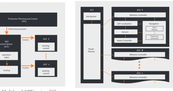
Automated Guided Vehicles (AGVs) represent autonomous machines whose purpose is to perform tasks, most likely transportation. The implementation of AGVs in the industry varies from hos-pitals (e.g. transportation of the laundry) to harbors [20]. AGVs are equipped with sensors and actuators and in most cases, they operate in a fleet manner. The general representation of the AGV system consists of coordinated autonomous guided vehicles. The main modules if this sys-tem is presented in Figure 3a and they are production planning and control (PPC) module, AGV control system (ACS) and the AGVs [20]. Communication between these modules is considered a part of the internal system. In Figure 3b detailed representation of AGV system is presented. ACS is in charge of assigning routes to each AGV and it plans optimal routes for AGVs. AGVs have behaviour controller (BC) which is making binary decisions and selects role-plays. BC is in direct communication with ACS and it sends success/failure messages.

(14)

Production Planning and Control (PPC) AGV AGV Control System (ACS) AGV n tracking control tracking control tracks internal processes tracks operation oders routing

(a) Modules of AGV system [20]

ACS Job planner Route- Planner Behavior Controller Behavior Controller Behavior Controller Self-Localization Navigation Path-Planner Trajectory-Generator Motor Controller Sensors AGV AGV n AGV

(b) AGV system overview [20]

Figure 3: AGV system properties

3. Related Work

To put this work into a broader context, compare it to current research and to expand an un-derstanding of a problem, we need to explore papers which are relevant to the topics covered in this thesis. Researching topics such as system-of-systems, AGVs, actor-based modeling and for-mal verification was conducted by searching through scientific databases such as IEEE Xplore and Scopus. Additionally, on the Publications section of the Rebeca website, there are several works closely related to the topic.

Direct correlation with works which include the Volvo Electric Site case study are [1], [6] and [7]. In [1] and [6], the AdaptiveFlow framework was explained in-depth and some examples for Electric Site case were provided. These papers show the applicability of the AdaptiveFlow through the example of this case. As the main difference from these papers, for this thesis, it is necessary to make a model of a suitable environment for the VCE Simulator scenario and in addition to that, we need to perform the mapping procedure from AdaptiveFlow to VCE Simulator. Jafari et al. [7] have performed formal modeling, using Timed Rebeca, and verification of fleet control system of autonomous haulers. The model proposed in this work uses a different perspective for modeling. More particularly, the machines on the site are perceived as actors, whereas in this project we are using the AdaptiveFlow principle of defining roads as actors and machines as messages sent between actors.

Modeling of self-adaptive systems has been introduced by Bagheri et al. [21]. In this paper, the focus was on Track-Based Traffic Control Systems (TTCS) with centralized control in which traffic flows through pre-specified sub-tracks. They have introduced a coordinated actor model which can be used to design self-adaptive TTCSs. Additionally, authors have proposed several mappings from different TTCSs to the coordinated actor model. However, this paper does not provide model checking solutions.

This work targets distributed systems and it is necessary to find relevant papers that are based on modeling and inspection of such systems. Distributed and asynchronous system modeling and analysis were done by Jafari et al. [22]. Due to the non-deterministic nature of these systems,

authors have used Probabilistic Timed Rebeca (PTRebeca) to perform modeling. They have

provided SOS rules for PTrebeca, presented a new toolset that generates Markov Automation from PTRebeca models in the form of the input language of the Interactive Markov Chain Analyzer (IMCA) [22]. Khamespanah et al. [23] conduct modeling of real-time Wireless Sensor and Actuator Network. They provide a very accurate view of WSAN application through actor modeling. In this work, authors have also used Timed Rebeca and Afra model checking tool.

Since this work deals with the case of collaborating AGVs, a few works on this topic have been extracted. Saddem et al. [24] targets path-finding algorithms in a 2D grid environment. They

(15)

have conducted their model-checking by using UPAAL Timed Automata. A similar problem was covered in [25], where authors inspect the automated planning of optimal paths for multiple robots. They have used weighted transition systems and Linear Temporal Logic (LTL) formula for the goal specifications. In this project, we have to adapt simulator scenarios and the behavior of machines in order to adequately perform the mapping. Authors in [20] have explored the main challenges when it comes to the distribution of knowledge and autonomy of AGVs. This work will provide a better understanding of the AGV system architecture. Transport assignments and collisions in AGV systems have been examined and verified by Weyns et al. [26]. The software architecture has been evaluated and through running the simulation, the test results were obtained. The authors have developed decentralized control architecture by applying Multiagent System (MAS).

In [27] mapping Robot Operating System (ROS) to Rebeca properties has been conducted. Furthermore, this work also examines the Volvo Electric Site case. The contribution of this work is the development of a mapping algorithm between ROS and Rebeca, therefore it proves possible verification of real robotic applications with Rebeca modeling language. The work is highly relevant since it has a similar purpose to this thesis and it is also based on the mapping procedure in which Rebeca is included. Differences reflect in that this thesis focuses on another way of mapping, from Timed Rebeca model to VCE Simulator and different perspectives have been chosen when it comes to modeling. In [27] actors were machines on the site, whereas in this work, due to the nature of the AdaptiveFlow, the roads are perceived as actors that exchange machines as messages.

Webster et. al. [28] introduce a case study of robotic assistants and their formal verification. The experimentation was done through verifying four sample properties of models that were trans-lated from Brahams into the input PROMELA modeling language. The case in this thesis covers the translation of system specifications defined in AdaptiveFlow to both, Rebeca models used for model checking and the Volvo Simulator inputs used for simulating the model. An additional difference is that our focus is on a collaborative system of multiple autonomous machines. In [29] there is a correlation with our project such that authors cover construction machines and their au-tomatization properties. The verification is performed with UPAAL. However, the main difference is that the subject of their research is an autonomous wheel loader and formal verification of its internal properties, whereas in our work the wheel loader is abstracted and is perceived as a part of a collaborative system. Zita et. al. [30] apply the formal verification to a specific module of autonomous vehicles. The lane change module was covered which is a part of the control system inside autonomous vehicles. Our work examines a track-based control system that directs machine movement in the quarry site.

(16)

4. Method

The goal of this thesis is to develop a technique for orchestration of several tools in order to evaluate and analyze collaborative systems of heavy machines. As a reference for choosing a suitable

method(s), H˚akansson [31] has provided a convenient overview of research methods generally used

in any kind of research that helped us in identifying the most suitable ones for this project. The initial point of this research is a hypothesis which states that AdaptiveFlow is useful for the model-driven development of the fleet management systems. Hence, our focus will be on quantitative research methods. This hypothesis will be measured through three cases whose experiments will be run on the Volvo Simulators and through model verification and evaluation. Through these experiments, the logs from the simulator will be used to extract the performance properties of the system. The models will also provide safety and performance information about the system by analyzing the state-space file generated from the model verification.

Data is collected through the model, as well as the simulation experiments. Besides, we have gone through three case studies in which tools have been used differently and have compared results from model checking and simulations for all three of them. Data collected has been analyzed by using statistical methods.

To ensure that this project is replicable and reliable we have provided detailed information about each case and how it was implemented. Each method and methodology has been shown through their applications in multiple activities during this project. Results gathered have been discussed and conclusions have been outlined.

4.1. Performed activities

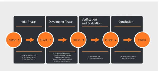
To answer previously mentioned research questions, defining an appropriate method for conducting this project is imperative. We have split the workflow into four phases which are shown in Figure 4, where each phase is validated.

The first phase of the project is focused on the understanding of the case which is being covered therefore, the background study was conducted. In this phase, it is necessary to understand what problems ought to be solved and how would it be done. In addition to that, the next step is the literature review in which relevant findings and contributions have been extracted.

The second phase consists of model design, mapping, and automatization of the mapping procedure. The first step is to analyze VCE Simulator and its properties. The next step is to generate the Timed Rebeca model, using the model generator from the AdaptiveFlow, by providing 3 input XML files (environment, configuration, and topology). These files are be modified based on what could be derived from the VCE Simulator. The environment.xml file has to be modified based on the terrain of the scenario in the VCE simulator. To assign points of interest (PoIs), such as parking station, charging station, and loading/unloading points, topology.xml file is specified. To define the configuration of the whole system we have to provide configuration.xml file. After that, it is necessary to identify mappable properties between AdaptiveFlow and VCE simulator. Lastly, the mapping procedure is developed and automatized.

The third phase is based on safety verification and performance evaluation. This is done by examining both, models as well as scenario representation of it in the VCE Simulator. Finally, in the fourth phase, the result analysis is performed by comparing results from model verification and the simulation, and finally, the conclusions are derived.

(17)

Initial Phase Developing Phase Verification_{and Evaluation} Conclusion

PHASE PHASE PHASE PHASE FINISH

1. Analysing VCE Simulator 2. Developing TRebeca Models

3. Mapping properties from AdaptiveFlow to VCE Simulator

4. Mapping automatization 1. Understanding the case

2. Background study

3. Literature Review 2. Performance evaluation

1. Analysis of given results 2. Drawing conclusions

Figure 4: Research Method

5. Mapping AdaptiveFlow Models to VCE Simulator Inputs

This section provides a description of each tool used for the verification and evaluation of the collaborative systems, as well as information on how the mapping was performed. First, we have

to go through the AdaptiveFlow framework. Each input file is described in detail because it

is necessary to understand all elements and their attributes. The workflow of AdaptiveFlow is provided to make a connection between defined input files, that provide system specifications, and model generating verification, and performance evaluation. Following that, the outline of the VCE Simulator is given. Mainly, the dynamic.content input file used for the definition of elements is explained to show a connection between this file and AdaptiveFlow’s environment, topology, and configuration files.

During this thesis, we have developed the VMap tool for automatic mapping. It can be seen as just another part of the orchestration which is used for faster development of desired simulation scenarios derived from AdaptiveFlow specifications. Its development, role, as well as the mapping pattern, is thoroughly described in this section.

5.1. AdaptiveFlow framework

AdaptiveFlow [1, 6] is an actor-based Eulerian framework which is used for a track-based flow

management system. Usually, when we think of actors in track-based systems, such as traffic systems, we would think of vehicles as actors. By making a parallel with fluid mechanics, this perception would be categorized as the Lagrangian view. In the AdaptiveFlow framework, we use the Eulerian view where the roads would be considered as actors and vehicles as messages sent between the actors. To explain the architecture of the AdaptiveFlow, first, it is necessary to explain in detail three files that are used for the system specification, as it is done did below.

5.1.1. AdaptiveFlow input files

The environment file

The environment.xml file is used for defining the base layer of the system, represented as a matrix, in which movement of the vehicles takes place [6]. The layer is split into segments that communicate with each other. Each segment is surrounded by neighboring segments and each neighboring segment is labeled based on the location relative to the current one (i.e. NE-northeast, SW-southwest, E-east, etc.). Segments also have unique identifiers, a capacity that usually assigns the number of vehicles that can be on the segment at the time and free speed which sets the allowed

(18)

speed for each segment in m/s. Coordinates of the segments are also defined. The example of the environment.xml file is presented below.

Listing 2: Example of the environment.xml file

The topology file

The topology.xml is used for assigning the locations of the points of interest (PoIs). PoIs contain unique identifiers, x and y coordinates, type of the point, and operating time. The PoIs can be perceived as key spots on which tasks are executed. An example of a topology file is shown below.

Listing 3: Example of the topology.xml file

The configuration file

To specify the system configuration the configuration.xml file (Listing 4) should be defined. It includes information such as the number of machines, resending periods for requests, safe distance between machines, policy for bypassing obstacles, fuel reserve of each machine, and the maximal number of allowed attempts to send a request to the unavailable segment before rerouting. The example part of the configuration.xml file for the system features is presented below.

(19)

The remaining part of the configuration file is adding machines and their properties. Each machine has tasks that are assigned as a set of IDs of PoIs. The attributes of the machines are unique identifiers, machine type, leaving time from parking station, fuel capacity, fuel consumption, speed, CO2 emission, capacity, and unloading time, as it is shown on Listing 5.

Listing 5: Example of the machine specifications

5.1.2. AdaptiveFlow workflow

AdaptiveFlow workflow is split into three phases. The initial phase is the pre-processing phase in which TRebeca models are generated by processing three input files (environment, configuration, and topology) with a Python script that represents the model generator. The next phase consists of formal verification of the generated model by generating the state space [1]. The verification is performed with model checking tools such as Afra or Rebeca Model Checker (RMC) [1]. These tools convert Rebeca models to C++ files which are afterward compiled to an executable file [1]. This file implements the model checking algorithm and it returns results. As mentioned before, model checking tools also generate state space of models used for the final, post-processing phase. In this phase, state-space goes through the Python script that analyses each state. The representation of the whole workflow is presented in Figure 5. Each phase of the workflow is described in-depth in the following sections.

environment.xml

topology.xml Python

script

OUTPUT

model.rebeca RMC statespace.xml Python

script

fuel consumptions material delivered operating time

emissions Pre-processing: model generation Model run and state-space generation Post-processing: state-space analysis

Figure 5: AdaptiveFlow workflow [1]

Phase 1: Pre-processing phase

In the AdaptiveFlow framework 3 input files are used for the system specification and those are environment.xml, topology.xml and configuration.xml.

After defining the elements of three input files, the next step is to run the model generator script which will derive the TRebeca model based on those input files. The representation of the model

(20)

could be designed as a matrix with PoIs. This representation is an abstraction of the scenario which excludes details of the system. The example of scenario depiction is shown below.

5 LUP 4 LUP 3 LUP 2 LUP CS1 0 PS 0 1 2 3 4 5 6 7 8 9 0 1 2 3 4 5 6 7 8 9

Figure 6: AdaptiveFlow environment [1]

Phase 2: Model run and state-space generating

In this phase, by using a model checking tool (either Afra or RMC) the model analysis is executed by generating C++ files from the input files. Compiling C++ files results in generating an executable

file. The execution of this file performs a model checking algorithm on the input model and

based on the results, the state space file is generated. Aside from checking regular properties such as deadlock-freedom and safety, AdaptiveFlow also verifies properties like fuel consumption of machines, correct machine movement, absence of machine collision with obstacles, and no-starvation property[6]. The generated state space file is used in the upcoming phase for extracting the performance properties.

Phase 3: Post-processing phase

The last phase of the AdaptiveFlow workflow consists of the evaluation of the performance prop-erties of the system through analysis of resulting, state space, file from the previous phase. The state-space file is analyzed with a Python script that extracts the evaluation of performance

prop-erties. The performance evaluation includes total CO2 emissions of machines, the amount of

consumed fuel, moved material, and operating time of the collaborative system.

5.1.3. Novel features of AdaptiveFlow

Throughout this thesis, AdaptiveFlow has been improved and upgraded in alignment with con-ducted project. New features that are implemented are proven as helpful when it comes to the mapping because these changes helped in developing more realistic cases.

With the new features of AdaptiveFlow, this framework now supports unidirectional routes, and users can specify directions between segments in the environment file. This means that even though segments are adjacent they are not necessarily linked. In Listing 6, specification of direction attribute of the segment element is presented.

(21)

Listing 6: Segment’s ”direction” attribute

An additional feature that was implemented is policy 4 and the routes element in the topology file. Since machines have tasks specified as a set of PoI IDs, the policy 4 specifies that the machines should follow the path between PoIs that is explicitly specified in routes element. The route element has attributes origin, destination and path. It is a sequence of segments that the vehicles must follow for reaching a PoI (destination) from the current PoI (origin). The values of origin and destination correspond to the ID of the PoI itself. The example of the routes element is shown in Listing 7. <t o p o l o g y> <POIs> . . . </POIs> <r o u t e s> <r o u t e o r i g i n=” 0 ” d e s t i n a t i o n=” 2 ” path=” s e g 8 7 , . . . , s e g 6 8 ” /> . . . . <r o u t e o r i g i n=” 0 ” d e s t i n a t i o n=” 3 ” path=” s e g 8 7 , s e g 7 8 , . . . , s e g 3 7 , s e g 2 8 ” /> </r o u t e s> </t o p o l o g y>

Listing 7: Defined routes in toplogy file

5.2. VCE Simulator

Volvo Simulators provide a real-life imitation of processes in Volvo construction sites. The features range from simulating the process of the individual machine to building up authentic scenarios [32]. VCE Simulator also provides data analysis of the scenarios in which users can evaluate the performance and efficiency of defined simulation models. In this case, we focus on the scenario building feature of the Volvo Simulators in which we build scenarios that are a convenient repre-sentation of the models. The simulation is used as an adjunct to the TRebeca models for system design, verification and evaluation.

For the scenario buildup, Volvo Simulators use a dynamic.content file as an input in which each object inside the simulation scenario is defined as an element in Extensible Markup Language (XML) format. In this file, we define elements such as edges, vertices, loading material, machines, etc. Our goal is to generate dynamic.content file according to the specification inside AdaptiveFlow inputs. The following section describes a tool developed to bridge a gap between the level of abstraction of AdaptiveFlow and VCE Simulator.

5.3. VMap: the conversion tool description

In this section, AdaptiveFlow is perceived as a design tool. Section 6.1. shows the case that has been examined in order to perform the analysis of VCE Simulator and AdaptiveFlow. De-scribed steps were necessary to derive mappable elements and based on that the tool for mapping automatization has been developed. The mapping automatization has been developed to bridge a gap between AdaptiveFlow specifications and VCE simulations and to complete model-driven development loop.

VMap is a tool developed in order to perform the mapping automatization from the Adaptive-Flow inputs (environment, configuration and topology) to the dynamic.content file that consists of static features for the simulator. These static features are an XML representation of elements inside the simulator scenarios such as vertices, edges, path points, automated haulers, loading machines, etc. What AdaptiveFlow provides us is a convenient method for design, analysis and verification of collaborative systems. The VMap tool has been developed with a goal to make a transition from an abstraction such as a TRebeca model to a concrete simulation of real-world scenarios. In addition to that, it is necessary to verify whether this transformation from TRebeca models to simulation provides correct-by-design scenarios. To conduct this transition in a valid way and to a full extent, it was essential to implement a logic that is a core of the AdaptiveFlow

(22)

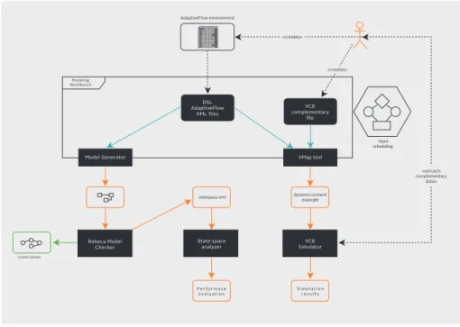
inside a Simulator. To illustrate all of the tools involved in orchestration process, including all of the inputs and outputs, we have designed a diagram shown in Figure 7. In upcoming sections, each part of the workflow is be thoroughly described.

AdaptiveFlow environment Input scheduling statespace.xml P e r f o r m a c e e v a l u a t i o n S i m u l a t i o n r e s u l t s dynamic.content example Modeling Workbench Counter Example 2LUP 3LUP 4LUP 5LUP 0PS 1CS <extracts complementary data> <creates> <creates> DSL AdaptiveFlow XML ﬁles VCE complementary ﬁle Rebeca Model Checker State space

analyzer SimulatorVCE VMap tool Model Generator

Figure 7: Tools used with their inputs and outputs

5.3.1. Development phases of modeling and conversion

Phase 1

The first phase consists of designing a suitable representation of the system. This includes designing the environment of the system, defining properties of machines and setting up the location of each PoI. When all of this has been set up, the next step is divided into two subbranches. The first branch includes defining AdaptiveFlow input files based on the desired requirements. Specified files will be used as inputs for two tools: Model Generator, which is a part of the AdaptiveFlow, and VMap. The second branch of the initial phase represents an extraction of complementary files for previously mentioned input files. The complementary file is extracted from dynamic.content file of scenarios inside the simulator and it differs based on the scenario. The contents of this file are all elements in the simulation which cannot be mapped directly from the AdaptiveFlow, such as camera elements, a base asset of the scenario, etc. Furthermore, the environment in VCE Simulator is represented in 3D, whereas in AdaptiveFlow we have a 2D representation of the environment. Since our goal here is to perform mapping and its automatization from an abstract 2D TRebeca model to a 3D environment in the simulator it would not be adequate to choose scenarios with the inconsistent and steep environment, therefore the scenarios with the relatively flat surface have been segregated.

Phase 2

The second phase is also split into two different sections. The first section, consists of the model generating, verification and evaluation, whereas the second section consists of the mapping from the defined environment to the VCE Simulator. The first section uses AdaptiveFlow input files for the model generation and goes through the whole process of AdaptiveFlow workflow. A first section is executed before the second one because it is necessary to first verify and evaluate the generated TRebeca model and then map model inputs to the Simulator.

(23)

The second section consists of a mapping procedure from AdaptiveFlow inputs to the VCE Simulator. In second part, AdaptiveFlow input files with the VCE complementary file, extracted in a previous phase, are used for generating two outputs. The first output file is an image that is a visual representation of a 2D environment that should be designed inside the Simulator. The second file represents a dynamic.content file example that shows how the input file in the Simulator is supposed to look like. It is used to define a suitable simulation scenario for the TRebeca model. Phase 3

In the final phase, the comparison of the results from two sections of Phase 2 is conducted. De-pending on the TRebeca model verification result, that result will be compared to the outcome in the simulator scenario. If the model checking results in dissatisfaction of checked properties, then that counter example will be mapped to the simulator to verify whether that scenario also fails there. Otherwise, if the model satisfies checked properties then the performance evaluation will be conducted and its results will be compared to the simulation results of the mapped model.

5.3.2. Description of files generated by the tool

The VMap tool is developed in Python programming language. It generates two output files that are dynamic.content example file and a guideline image which is an abstracted illustration of the desired Simulator scenario represented in 2D. Generated two files are then used to develop a suitable simulation scenario. At the current stage of development, the dynamic.content example file is used as a proof of concept. This is the case because there are several attributes in the certain XML representation of objects that could not be assigned externally.

VCE Guideline

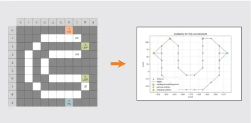
Referring back to the previous explanation, the guideline image, generated with the script, is a representation of the AdaptiveFlow specifications in VCE Simulator fashion. This image can be used as an instruction for developing an adequate simulation scenario by converting AdaptiveFlow segments into edges and vertices defined in the script. In addition to that, information from the topology file is extracted to place each PoI to a vertex which is in that PoI location. In shown image, each PoI is labeled relative to its type. The coordinate plane of represented image is calculated based on a scenario. The starting and ending coordinates are extracted from the simulation scene and after that, the coordinate plane is split into a 10x10 grid to equalize it with the AdaptiveFlow segmented environment. After that calculation, each vertex is put on the midpoint of every available segment and every vertex has a directed edge towards those vertices to which that segment is directed to. Identified connections stand for edges in the simulation terms. In Figure 8, for the illustration purpose, we show the transformation from the AdaptiveFlow environment of scenario described in previous sections to the 2D Simulator representation.

(24)

The dynamic.content example

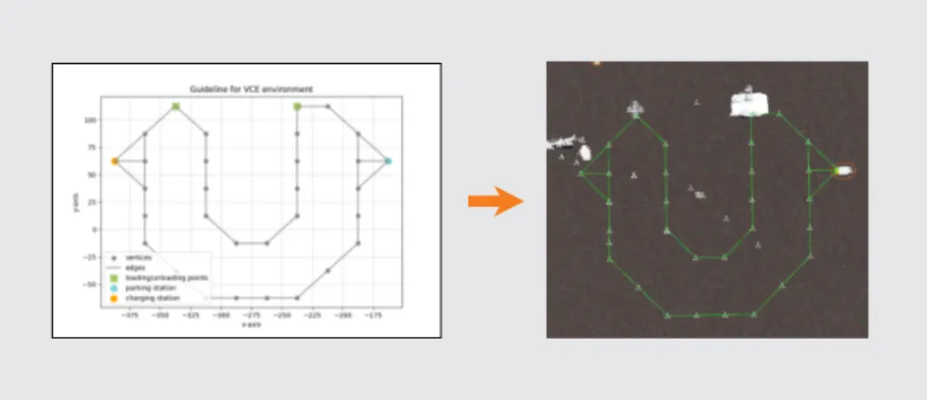
The VCE Simulator uses a dynamic.content file for each scenario which is an Extensible Markup Language (XML) representation of every element, its attributes and their communication. Based on the information from this file every element is properly set up inside the scenario. The other file that is generated with the VMap tool is dynamic.content example file. It used as a proof of concept which tells us that the AdapiveFlow input files could be mapped directly and automatically with the VMap tool. The only obstacle/limitation in running the dynamic.content file, generated by the tool, directly inside the simulator is the generating of persistentID for each new element created. The VCE Simulator has a specific method for generating this attribute which could not have been accessed. Despite that, the VMap tool can be used with the Rebeca tool stack and VCE Simulator in a combination to perform formal verification of collaborative systems, moreover, it can be observed as a link between the two. For now, this file in a combination with an image file, generated by the VMap tool, is used as instruction files to develop a suitable simulation scenario based on the AdaptiveFlow specifications by using VCE Simulator’s Scene Editor. Figure 9 shows an example of how the elements can be generated directly inside the simulator just by strictly following the outputs of the VMap tool.

Figure 9: Scenario developed by following the guideline

5.4. Conversion of elements from AdaptiveFlow to VCE Simulator

This section gives an in-depth description of elements that were identified as mappable from Adap-tiveFlow to VCE Simulator. The conceptual, as well as applicative description of the mapping pattern, was presented to better grasp how the mapping pattern has been defined and to provide a better understanding of how the VMap tool for mapping automatization, described in section 5.3. has been developed.

The main elements that have been mapped from AdaptiveFlow to the Volvo Simulator are segments and PoIs. The attributes of elements such as speed, capacity, length, type, etc. have been mapped to the Edge element of the input file for the Simulator. Newly developed route element from AdaptiveFlow has been mapped to the AhMission in the Simulator’s file in which we define machine paths (missions). As for the machines, AdaptiveFlow provides more specific information than the Simulator. Attributes such as leavingTime, unloadTime and speed are related to the same attributes of the Simulator’s Edge element. However, other information could not be used in the Simulator’s input file, since attributes like fuelConsumption or emission have not yet been implemented. The system element in AdaptiveFlow specification represents a very convenient way of specifying system properties of fleet management, but only safe distance, number of vehicles and policy could be mapped to the VCE Simulator. As for the policies, policies for rerouting and bypassing obstacles are yet to be implemented in the simulation.

(25)

5.4.1. AdaptiveFlow environment

As previously noted, the environment in the AdaptiveFlow is split into segments that communi-cate with each other, by sending machines as messages. Defined segments represent tracks through which machines travel. Each segment is represented as an actor that includes additional attributes such as allowed speed, segment length, capacity, etc. To derive the mapping pattern, the track rep-resentation inside VCE Simulator needs to be identified. The track reprep-resentation in the simulator consists of multiple components that have been described below.

• Vertices – This element is identified in the initial scenario, but it is not considered as essential for a mapping.

• Edges – The edges are elements which consist of path points and a script that represents logic for the edge control. There are also dynamic properties such as poiType, speed and capacity that were subsequently implemented and defined in examined cases based on attributes of the AdaptiveFlow segments.

• EdgeControl – This component represents a script in which edge is being controlled by certain attributes. This script has been implemented in Section 6.1. of reverse engineering and it is based on the logic of AdaptiveFlow in which all edges are controlled.

• PathPoints - All edges consist of path points that machines are following when they are moving through edges.

Segments from the AdaptiveFlow have been mapped to the several elements described above.

All of the segments can be transformed into path points and edges. In the defined mapping

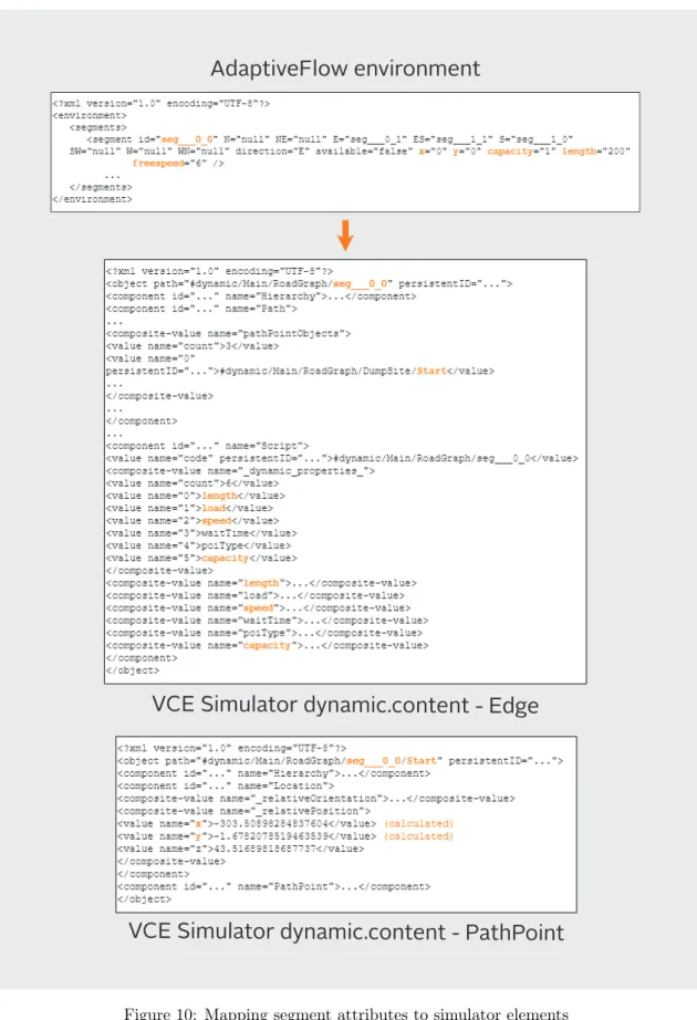
pattern, in the middle point of each segment, the path point is put. Adjacent segments, which have defined paths between them by assigned directions in AdaptiveFlow, are connected with edges. For example, if there are segments A and B and if the direction in environment.xml file is defined as from A to B, by using this mapping pattern, the result would be 2 PathPoints in the middle of both segments and one Edge that represents the connection between these two points. It is important to note that in the mapping procedure, the starting point of the edge is located at the center of that segment and the ending point is located in the middle of the adjacent segment to which the current one is connected to. The new representation could be also defined as a graph. For this case, the environment in AdaptiveFlow is illustrated as a graph G, vertices are PathPoints defined as Pi = (Xi, Yi) by which Edge lengths is derived as a cost matrix E = (eij). The Edge

element length eij is Euclidean distance between PathPoints which is formulated as in Equation

4.

eij =

q

(Xi− Xj)2+ (Yi− Yj)2 (4)

Segement attributes, such as capacity and allowed speed are defined in the Edge component and are controlled in the EdgeControl script.

(26)

AdaptiveFlow environment

VCE Simulator dynamic.content - PathPoint

VCE Simulator dynamic.content - Edge

(27)

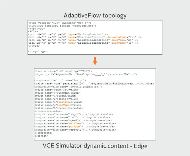
5.4.2. AdaptiveFlow topology

Since current implementation inside the simulator did not have defined edge types by which it could be determined whether one edge is loading track, unloading track or parking track, we had to make that implementation to develop a convenient mapping pattern. In the AdaptiveFlow, a topology file contains information about PoIs. The current state of the implementation sup-ports the most essential PoIs which are Parking Station, Charging Station and Loading/Unloading point. Additionally, the information about the x and y coordinate of that PoI in the segmented environment is also defined. Based on that, we can see to which segment that PoI belongs to.

Taking this into consideration, the PoI information was perceived just like additional informa-tion to specific segments. New attributes depend on the PoI type, so for the Loading/Unloading point there is an additional loadTime attribute and for the Charging Station there is a charging-Time. In the simulator’s dynamic.content file added attributes were merged to an Edge object. Newly defined attributes are poiType and waitTime. In the Figure below we can see how mentioned attributes are converted.

AdaptiveFlow topology

VCE Simulator dynamic.content - Edge

Figure 11: Mapping PoI attributes to simulator Edge attributes

5.4.3. AdaptiveFlow configuration

A final module that is mapped from the AdaptiveFlow is the system configuration. The configu-ration is divided into two parts: system and machines. In the system specification, the elements that were recognized as mappable are the number of vehicles and safe distance between machines. The number of machines is not explicitly specified inside the dynamic.content file but we can define as many machines as we need. The safe distance between machines is specified in meters and this property is mapped to the GraphicalField component inside the machine element in the

(28)

dynamic.content file. It represents the range around the machine which could be considered as a safe zone. If the obstacle appears inside the zone the machine will automatically stop.

Obstacle Autonomous hauler

GraphicalField (safety zone) EllipseOutline

Figure 12: Machine safety zone

The second part is the machine specification. For attributes such as fuelCapacity, fuelConsump-tion, emmision and capacity we do not have equivalent attributes implemented inside machine objects in the VCE Simulator. Regardless, the machine attributes in AdaptiveFlow such as leav-ingTime and unloadTime is attached to the edge object in dynamic.content file. The final mapped machine property is machine tasks. This property is connected to the routes from the topology file in AdaptiveFlow in which PoIs are also defined. Machine tasks are specified as a set of PoI identifiers and inside the routes element we set up paths between PoIs. Those paths represent a set of segments through which machines go in order to reach their destination. The combination of machine tasks and routes results in the mapping to the simulator’s AhMission object inside the machine. The AhMission is a set of edges that defines a full path that the machine has to follow for the purpose of executing its tasks. In Table 1 a mapping pattern of each element and their attribute is presented.

Tool orchestration for modeling, verification and analysis of collaborating autonomous machines

V¨

aster˚

as, Sweden

Thesis for the Degree of Master of Science (60 credits) in Computer

Science with Specialization in Software Engineering

TOOL ORCHESTRATION FOR MODELING,

VERIFICATION AND ANALYSIS OF

COLLABORATING AUTONOMOUS

MACHINES

Pavle Mrvaljevi´c

pmc19001@student.mdh.se

Examiner: Antonio Cicchetti

M¨

alardalen University, V¨

aster˚

as, Sweden

Supervisors: Marjan Sirjani and Anas Fattouh

M¨

alardalen University, V¨

aster˚

as, Sweden

Company supervisor: Stephan Baumgart

Volvo CE, Eskilstuna

Table of Contents

List of Figures

1.

Introduction

1.1.

Problem Formulation

1.2.

Research Questions

1.3.

Research Contributions

2.

Background

2.1.

Model-Driven Development

2.2.

Formal Methods

2.3.

Actor model

2.4.

Rebeca Modeling Language

2.5.

Volvo Electric Site

2.6.

Automated Guided Vehicles - Distributed Systems

3.

Related Work

4.

Method

4.1.

Performed activities

5.

Mapping AdaptiveFlow Models to VCE Simulator Inputs

5.1.

AdaptiveFlow framework

5.2.

VCE Simulator

5.3.

VMap: the conversion tool description

5.4.

Conversion of elements from AdaptiveFlow to VCE Simulator

AdaptiveFlow environment

VCE Simulator dynamic.content - PathPoint

VCE Simulator dynamic.content - Edge

AdaptiveFlow topology

VCE Simulator dynamic.content - Edge