Investigating the performance of matrix factorization techniques applied on purchase data for recommendation purposes

(1)

Investigating the performance of

matrix factorization techniques

applied on purchase data for

recommendation purposes

Master Thesis project

Author:

John Holl¨

ander

Supervisor:

Prof. Bengt J Nilsson

(2)

Contact information

Author:

John Holl¨ander

E-mail: johnchollander@gmail.com

Supervisor:

Bengt J Nilsson E-mail: bengt.nilsson.ts@mah.se

Examinor:

Edward Blurock E-mail: edward.blurock@mah.se

(3)

Abstract

Automated systems for producing product recommendations to users is a relatively new area within the field of machine learning. Matrix factor-ization techniques have been studied to a large extent on data consisting of explicit feedback such as ratings, but to a lesser extent on implicit feed-back data consisting of for example purchases. The aim of this study is to investigate how well matrix factorization techniques perform compared to other techniques when used for producing recommendations based on purchase data. We conducted experiments on data from an online book-store as well as an online fashion book-store, by running algorithms processing the data and using evaluation metrics to compare the results.

We present results proving that for many types of implicit feedback data, matrix factorization techniques are inferior to various neighborhood-and association rules techniques for producing product recommendations. We also present a variant of a user-based neighborhood recommender sys-tem algorithm (UserNN), which in all tests we ran outperformed both the matrix factorization algorithms and the k-nearest neighbors algorithm re-garding both accuracy and speed. Depending on what dataset was used, the UserNN achieved a precision approximately 2-22 percentage points higher than those of the matrix factorization algorithms, and 2 percent-age points higher than the k-nearest neighbors algorithm. The UserNN also outperformed the other algorithms regarding speed, with time con-sumptions 3.5-5 less than those of the k-nearest neighbors algorithm, and several orders of magnitude less than those of the matrix factorization algorithms.

(4)

Popular science summary

As a shop owner, how does one figure out what products other people prefer or need? How do you decide what present to buy for your friend, or perhaps recom-mend a customer if you are a sales person? For the last decades, these questions have not solely been pondered upon by sales people, advertising agencies, and present buyers. Nowadays, there are computer scientists studying techniques for how computers can find out and recommend the products most likely to suit the customers needs and desires. Especially when we shop online, the data from our clicks and purchases are stored and available for processing. Just as humans, computers can be taught to find patterns in how we make our decisions while shopping.

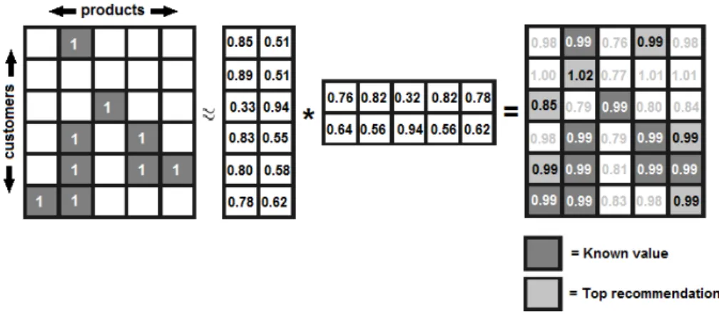
There are several techniques for finding these patterns. Some involve com-paring the customers’ clicks and purchases and basing recommendations on what similar customers bought. Other techniques look upon what items are often clicked on or purchased by the same customers, and recommend products connected to those the customer has already shown an interest in. There is also the technique called matrix factorization, which is a more general mathe-matical approach for finding the patterns. This technique has been popular for predicting movie ratings, but has not been studied as much for making recom-mendations based on purchase data. As the name reveals, matrix factorization involves representing the data as a matrix, with the rows representing products and the columns representing customers. On every occasion a customer has bought an item, the number 1 is filled in the index of that customer and item.

Figure 1: Producing recommendations using matrix factorization.

(5)

recommendations. The left one of two smaller matrices in the middle repre-sents latent user interests and the right one reprerepre-sents latent product interests. Multiplying each row in the left matrix with each column in the right matrix results in recommendation-values for all products to all customers. The higher a recommendation-value is, the stronger is the indication that the product is a good recommendation for the corresponding customer.

Some might ask, why would this method work? The answer is that the pro-cedure captures the pattern of the rows and columns from the original matrix and use the pattern to fill in the missing values. However, there are a lot of different factors to adjust in making the results as accurate as possible. The accuracy can also vary depending on how much data the matrix contains.

In this study, we have performed experiments regarding how well matrix factorization works for recommending products when processing data consisting of purchases. We compared the results produced by matrix factorization to those produced by other techniques. What we found out was that on the purchase data we used in our experiments, various other techniques produced more accurate recommendations than matrix factorization.

One of the techniques which outperformed the Matrix factorization tech-niques was the user-based neighborhood model. In a user-based neighborhood model, the recommendations to a customer are based on purchases made by other customers with a similar purchase history.

The other technique which outperformed the matrix factorization techniques was the association rules model. In this technique, one looks at how strong the connection is between products. If two products are often purchased by the same customers they have a strong connection. The recommendations to a cus-tomer are products with strong connections to the ones the cuscus-tomer already purchased.

We performed the experiments on data from two online stores namely a book store and a fashion store. The top performing technique regarding the bookstore data was a variant of a user-based neighborhood model which we developed. It performed approximately 9-22 percentage points more accurate recommendations than the two matrix factorization techniques we tested. On the data from the fashion store, the association rules model was the best per-former producing recommendations approximately 2-4 percentage points more accurate than those of the matrix factorization techniques.

(6)

Acknowledgements

I hereby express my gratitude towards the many people who have participated in the completion of this project.

I wish to thank PhD student and co researcher Dimitris Paraschakis for his participation and ample contribution throughout the whole research process.

I offer my gratitude towards my supervisor Prof. Bengt J Nilsson and Dr Natalie Schluter for their very valuable sharing of knowledge in the field as well as advice regarding the research and writing of this thesis.

My thanks also go towards Dr Annabella Loconsole and Dr Edward Blurock for their advice and feedback on the thesis work.

This project would not have been possible without the cooperation of the people at Apptus technologies. My gratitude goes towards Mikael Hammar and Jonathan Wulcan for the help in and sharing of knowledge, Bj¨orn Brod´en for helping me optimize the speed performance of the UserNN algorithm as well as giving me an insight in how Apptus recommender systems work.

Last but not the least I wish to thank my family for their very valuable support throughout my studies.

(7)

List of Figures

1 Producing recommendations using matrix factorization. . . iii 2 Approximation of R. R ≈ P × QT _{= ˆ}_{R. . . .} ₁₆

3 Overfitting represented by a polynomial function. The function passes through each data point yet represents the data pattern very badly due to the extreme values. . . 18 4 Underfitting represented by a polynomial function. The patterns

of the data are not represented accurately as the function misses the data points to a large extent. . . 18 5 A regularized polynomial function. It captures the pattern of the

data by passing through each data point without containing any extreme values. . . 19 6 A polynomial function representing the results of using dimension

reduction. The function represents the data pattern better than the one containing more factors as demonstrated in figure 3. MF recommender algorithms use dimension reduction in conjunction with regularization in order to minimize under- and overfitting. . 20 7 Mean Average Precision. . . 22 8 Original dataset format (the numbers are fictional). . . 33 9 Converted dataset format (the numbers are fictional). . . 34 10 Splitting the original dataset and evaluating the

recommenda-tions. The green dot represents a recommendation that corre-sponds to an actual purchase in the test set. . . 36 11 Golden section search. . . 39

(10)

List of Tables

1 The datasets. . . 33 2 Dataset01; training - and test set figures. . . 37 3 Dataset02; training - and test set figures. . . 37 4 Parameter values gained from the GSS optimization. Note; the

WRMF needs less iterations than the BPRMF since it updates one of the matrices P and QT at a time hence solves the approx-imation optimization quadraticly. . . 41 5 The results of all algorithms run on dataset01. . . 42 6 The results of all algorithms run on dataset02. . . 42 7 Processing time consumptions. In a colored version of this report,

the overall best results are colored blue, and the best performing MF algorithm’s results are colored red. . . 43

(11)

Notation

Abbrevations

ALS Alternating Least Squares.

AveP Average Precision.

BPRMF Bayesian Personalized Ranking Matrix Factorization.

CF Collaborative filtering.

MAP Mean Average Precision.

MF Matrix factorization.

MMMF Maximum Margin Matrix Factorization.

prec@n Precision at the n top recommendations.

recall@n Recall at the n top recommendations.

SGD Stochastic gradient descent.

WRMF Weighted Regularized Matrix Factorization.

(12)

Variables

L(u) List of recommendations to the user u.

T(u) List of items observed by the user u.

R, R A Matrix R. Q A Matrix Q. P A Matrix P . U A Matrix U . V A Matrix V . Σ A Matrix Σ. ˆ R An approximation of matrix R.

k The k-rank value.

ui The i-th user.

ii The i-th item.

ri The i-th row of a matrix R.

rj The j-th columns of a matrix R.

rij The element at row i and column j in a matrix R.

(13)

1 Introduction/background

With the pervasity of e-commerce systems, which are generally not burdened by typical commercial physical constraints, today’s consumers face a vast variety of choices among products to choose from. In the process of finding the products most suited to their needs and desires, it is virtually impossible to examine more than a fraction of everything offered on the market. Small businesses ideally strive to present products that hold a high probability of fulfilling the consumers needs and desires in order to not only increase sales but also enhance consumer satisfaction. To this end, recommender systems have been developed with the purpose of predicting which products hold a high probability of matching the consumers individual tastes, needs or requests.

There are numerous techniques used in recommender systems; they can how-ever be divided into two main categories, namely collaborative and content-based filtering. Content-content-based filtering techniques take item-content into ac-count as they build models based on item-features in combination with user interest[1, 2]. Collaborative filtering (CF) is defined as methods that produce recommendations based on patterns extracted from already existing user ratings or user actions (for example purchases) [2]. CF is also divided into two cate-gories which are user-based and item-based CF, both of which we have tested in the experimental process. Apart from these two categories, there is also a more general and mathematical approach called Matrix factorization(MF). This research will focus on using MF techniques on purchase data containing unrated products.

We have carried out the research process in cooperation with Apptus Tech-nologies1, a company that provides recommendation systems to customers in the e-commerce trade. Apptus Technologies have to date not implemented MF techniques in the recommender systems they develop. The datasets used in this study consist of purchase data from two of Apptus customers, one online book-store and one online fashion book-store. They are very sparse and consist of almost binary data. This differs from the data used in other studies described in this thesis, which is why our study is of value both Apptus Technologies and the computer science world in general.

(14)

1.1 Research contribution

Regarding rating predictions, collaborative filtering has been studied to a large extent[3]. On the other hand, datasets that consist of purchase data instead of ratings deserve further research. This in order to enhance knowledge about how recommender systems can be used and developed to provide satisfying recommendations despite the absence of ratings. Pradel et al.[3] focuses on datasets from one branch and one company namely Boˆite `a Outils (BAO), which is a home improvement retailer. The fact that their data comes from physical stores as opposed to online stores implies a significant difference, as it results in a different shopping behavior. The data used in the Pradel study is also relatively dense having a sparsity of 94.3 %, as opposed to the data we used, having sparsity levels of 99.9985 % resp. 99.9361 %. Apart from the these differences between the datasets, the difference between the types of products they consist of is also an important factor.

Another study that has researched recommendations based on data in ab-sence of ratings is that of Aiolli[4], in which the tests are performed on the million songs dataset. The sparsity of the million songs dataset is 99.99 % hence very high as in the datasets we use. However, the data differs from that used in our study as a user’s song listening history reveals more about user preference than product purchase history does.

Our study also aims at filling a gap for Apptus Technologies. The main contribution of our research is about applying known techniques on new sets of data. We have also contributed by presenting a variant of a user-based neighbor-hood recommender system algorithm. We have used it as one of the baselines, comparing its performance to those of the matrix factorization algorithms.

As our hypothesis in section 1.3 states, we predicted a negative result since a general mathematical approach such as matrix factorization is more dependant on the density of the data than various other approaches. In addition, the data we use is implicit and would to a large extent consist of 0’s and 1’s even if we had not converted it to binary. The challenges these characteristics pose sub-stantiates our hypothesis. This because Matrix factorization seems less suitable for implicit feedback data unless modifications have been made[4, 5]. Data that is close to, or completely binary, leaves less room for modification as it is harder to interpret in an explicit manner.

(15)

1.2 Research question

From the research gap identified we have derived the following research question: With what level of performance can collaborative filtering using matrix factor-ization techniques produce product recommendations based on various purchase data?

1.3 Hypothesis

From our estimates regarding the outcome of this research as described in the introduction, we have extracted the following hypothesis: Matrix factorization techniques can not produce satisfactory results as compared to other CF algo-rithms when used for producing product recommendations based on purchase data.

1.4 Goals

The following goals are the primary ones for our research.

• To find out the level of performance at which collaborative filtering us-ing matrix factorization techniques can produce product recommendations based on various purchase data.

• To find out which matrix factorization technique has the best performance for producing product recommendations based on various purchase data.

(16)

2 Preliminaries

2.1 Collaborative filtering

As mentioned in the introduction, CF is defined as methods that produce rec-ommendations based on patterns extracted from already existing user ratings or user actions (for example purchases)[2]. The benefit of using CF techniques in recommender systems is that it enables personalized recommendations as it learns the patterns from historic data. Another benefit of CF is that it is domain-independent, as it doesn’t take content into account.

A drawback of CF techniques is that they suffer from the cold start problem. The cold start problem occurs when little or no historic data in which to find patterns is available.

2.2 Implicit feedback

The type of data in the datasets that recommendation systems run on is di-vided into two categories namely implicit and explicit feedback. A feedback is referred to as implicit when it consists of indirect feedback for example a pur-chase or a viewed movie. Explicit feedback refers to when customers provide direct feedback in terms of ratings. A factor that exists in both explicit and implicit feedback is noise. In datasets used by recommender systems, noise can be viewed upon as misleading values that may affect the prediction accuracy negatively. The noise factor in implicit datasets is explained further down in this section. The datasets we use in our research consist of purchase data and thereof implicit data. Due to the unique characteristics of implicit feedback data, one cannot directly use the algorithms designed for running on explicit feedback data[5]. The study by Hu et al.[5] provides a comprehensive explana-tion of these characteristics. A shortened version of their explanaexplana-tion is provided below.

• No negative feedback. By observing the users’ behavior, we can infer which items they probably like and thus chose to consume. However, it is hard to reliably infer which items a user did not like.

• Implicit feedback is inherently noisy. An item may have been purchased as a gift, or perhaps the user was disappointed with the product. These circumstances can mislead a recommender system into incorrectly inter-preting a value in the dataset as an indicator that a user likes a product. That interpretation may be a falsity.

• The numerical values of implicit feedback indicate confidence, unlike the values in explicit feedback which indicate preference. The value

(17)

indicat-ing confidence in implicit feedback represents the frequency of actions for example how many times a customer bought a product. A high numeric value might not necessarily represent how much the customer likes the product, on the other hand a product only bought once might be the customers favorite product.

• Evaluation of implicit feedback recommender systems requires appropriate measures. Unlike with models running on user rated items, with models based on implicit feedback we have to take into account availability of the item, competition for the item with other items, and repeat feedback.

2.3 Fundamentals of Matrix factorization

The use of MF in recommender systems is a widely researched area. The basic principle of MF is that by decomposing a matrix R into two(in most cases) matrices one gains one matrix P containing user- features and one matrix QT

containing item-features. These features are also known as latent factors. The objective of MF - techniques when used in collaborative filtering is to obtain a matrix ˆR from the product of QT _{and P . An approximation of R is reached}

once it to a certain level resembles matrix R regarding the known values, but also contains approximations of the missing values. These approximations are the rating predictions when using explicit feedback data. When using implicit feedback as we do in our research, the missing value approximations are the basis for the recommendations.

Figure 2: Approximation of R. R ≈ P × QT = ˆR.

There are several different MF techniques often implemented with modifica-tions or optimizamodifica-tions. MF techniques have proven to be superior for producing product recommendations, compared to classic nearest-neighbor techniques[6], at least when running on datasets consisting of explicit feedback. They do how-ever have the drawbacks of being time-consuming to compute and less favorable

(18)

to run on implicit feedback datasets unless modifications have been made[4, 5]. This due to the fact that implicit feedback data lack information about the users’ interest in the product, as opposed to explicit feedback data which con-sists of ratings.

The SGD and ALS techniques described in section 2.5.1 and 2.5.2 are widely used in MF recommender system algorithms. They are also the basis of the state of the art MF algorithms which performed best in our tests. For the reasons mentioned above we have chosen to describe them in this thesis.

2.4 Data approximation

When used in the field of recommender systems, matrix factorization techniques are all about data approximation. This section explains some fundamental prob-lems concerning data approximation from the perspective of matrix factorization techniques.

2.4.1 Overfitting

When adjusting matrices P and QT _{in order to approximate matrix R, merely}

considering how well ˆR and R match regarding the known values is in most cases insufficient. As the process attempts to match the known values, the unknown values stray to extremes not representing a usable approximation of R. In the field of MF, this is denoted as overfitting. Overfitting can be suppressed by taking different measures such as regularization and dimension reduction, described in section 2.4.3 and 2.4.4.

(19)

Figure 3: Overfitting represented by a polynomial function. The function passes through each data point yet represents the data pattern very badly due to the extreme values.

2.4.2 Underfitting

An approximation is denoted as underfitted if the patterns of data is not pre-served to a satisfactory extent. In other words, underfitting is when the approx-imations level of accuracy is insufficient.

Figure 4: Underfitting represented by a polynomial function. The patterns of the data are not represented accurately as the function misses the data points to a large extent.

(20)

2.4.3 Regularization

The concept of regularization is to decrease the influence of the latent factor vectors in a way that prevents overfitting. In MF algorithms, the level of regu-larization is controlled by a constant λ which if given the correct value prevents overfitting yet avoids underfitting.

Figure 5: A regularized polynomial function. It captures the pattern of the data by passing through each data point without containing any extreme values.

2.4.4 Dimension reduction

Dimension reduction implies reducing the number of factors in the two matrices gained from decomposing the original matrix. A variable K denotes the number of dimensions which to keep. As the prediction performance of a recommender system using MF techniques is reliant on the K-value, it is crucial to choose an optimal value for it. The objective is to find a K-value that is large enough to preserve the patterns of the matrix yet small enough to avoid overfitting[7]. An optimal K-value can be found by testing different values in an experimental approach[7].

(21)

Figure 6: A polynomial function representing the results of using dimension reduction. The function represents the data pattern better than the one con-taining more factors as demonstrated in figure 3. MF recommender algorithms use dimension reduction in conjunction with regularization in order to minimize under- and overfitting.

There are different approaches regarding how to determine the optimal number of factors. One approach is to use Singular value decomposition, as described in [7]. In our study, we determined the optimal number of factors using the Golden section search optimization process described in section 5.3.

2.5 Matrix factorization techniques

2.5.1 Stochastic gradient descent(SGD)

The fundamental approach for Stochastic gradient descent is to achieve ˆR by iteratively update the values in P and QT_{, calculating their product ˆ}_{R and}

comparing it to R. The difference(error) between R and the product of P and QT is denoted e, and is calculated for all rij, by comparing all rij to the product

of its corresponding vectors pikin P , and qkjin QT. The update of pikand qkj,

taking e into account, is performed in every iteration by the following update formulas retrieved from [8]:

p

0_ik

= p

ik

+ η · (e

ij

· q

kj

− λ · p

ik

)

(22)

The variable η is the learning rate, which is a predetermined constant affect-ing the magnitude of the update steps. The other variable λ is the regularization constant explained in section 2.4.3.

This iterative update process continues until ˆR ≈ R regarding the known values.

2.5.2 Alternating Least Squares(ALS)

ALS is similar to SGD with the exception that instead of updating the values in both P and QT on every iteration, the values in P are fixed when solving QT and vice versa. In other words, there is an alternation between updating the user factors and item factors. This allows for an optimal solving as it makes the optimization problem quadratic[2]. In other words, the function of a quadratic optimization problem has only one maximum or minimum hence no other local maximums or minimums to be misinterpreted as optimal.

2.6 Evaluation metrics

2.6.1 Precision and recall

Two commonly used metrics in evaluating recommender systems are precision and recall. Precision can range from 0 to 1. Given a list of recommended items, precision denotes the proportion of them to be considered true recommendations as they were actually bought by the users. For example if the precision is 0,09, it means that 9% of the recommended items in a list L(u) correspond with the purchased items T (u). Accordingly, the higher the values of precision and recall are, the better the performance.

Recall can just as precision range between 0 and 1. Given all purchases T (u), recall denotes the proportion of them that are listed among the recommended items L(u). If the recall value is 0,09, it means 9% of the items purchased are also listed among the recommendations.

The equations of precision and recall retrieved from Kantor et al.[2] are listed below.

Precision(L) =

_{|U |}1

P

u∈U

|L(u) ∩ T (u)|/|L(u)|

Recall(L) =

_{|U |}1

P

u∈U

|L(u) ∩ T (u)|/|T (u)|

Since precision and recall are both very important as well as usually used in conjunction, there is a metric involving both of them called F1. F1 takes both precision and recall into account and weighs the conjunction of them towards

(23)

whichever of their values is the lowest.

F1 = 2 ·

precision · recall

precision + recall

2.6.2 Mean Average Precision

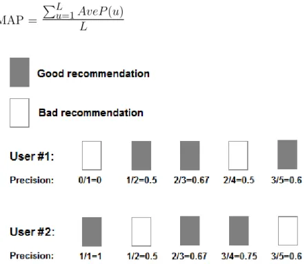
P. Kantor et al. also states that given a list of recommendations L(u) for a user, precision and recall does not distinguish the difference in relevance of these recommendations, which make them all look equally interesting to the user. We therefore used an additional metric called Mean Average Precision (MAP), which takes the ordering of the relevant items in the list of recommen-dations into account as well. In order to calculate the MAP one must first calculate the Average Precision (AveP). The MAP is the average of the average precisions of all the users’ recommendations as illustrated in figure 7.

MAP =

P

L

u=1

AveP (u)

L

(24)

3 Literature review

The literature revised in this section concerns the main two types of datasets on which recommender systems run. The type of datasets most related to our research are implicit feedback ones about which related studies are revised in subsection 3.1. As the most extensive research in the field of recommender systems concern explicit feedback, a few studies regarding such are also worth revising as is done in section 3.2.

3.1 Recommendations based on implicit feedback datasets

A study closely related to ours is that of Pradel et al[3], in which different collab-orative filtering techniques are tested on purchase data provided by La Boˆite `a Outils (BAO), a retail chain that sells products for home improvement. Matrix factorization among other collaborative filtering techniques are tested regard-ing accuracy in recommendregard-ing products to customers. Regardregard-ing the non-MF techniques, they apply item-based ones exclusively and concludes that bigram association rules obtained the best performances in their study. This in con-trast to results on rating data where neighborhood and matrix factorization are among the best performing methods[6]. They also state that different contex-tual factors such as purchase recency may have at least the same importance as the choice of algorithm. Importantly the study by B. Pradel et al concludes that recommender systems can be developed on purchase rather than rating data.

Aiolli[4] researches a recommendation-system for very large scale binary datasets. The dataset they run it on is called the Million Song Dataset. The study by F. Aiolli is similar to ours in the sense that the dataset they run the recommendation system on consists of implicit feedback. The dataset is very sparse as the fraction of non-zero entries (a.k.a. density) is only 0.01%. The algorithms implemented in the study of F.Aiolli resembles the known neighbor-based technique used for explicit feedback data. They mention several reasons for not using MF techniques despite the fact that as they state, it is considered a state of the art among CF techniques[4]. One of the reasons is that running MF calculations on large datasets is very time-consuming. Another reason they mention is that MF is typically modeled as a regression problem and therefore not suitable for implicit feedback tasks unless some modifications to the original technique are implemented[4, 5]. The main result of the study by F. Aiolli they state is a technique which applies well on very large implicit feedback datasets. Both item-based and user-based techniques are used. In the circumstances re-garding their choice of algorithms and datasets, user-based techniques produce the most accurate recommendations.

(25)

In another study by Hu et al.[5] they model a TV show recommender engine. The dataset consists of implicit feedback from the viewers of the TV shows. Since MF techniques have proven to achieve great results they construct a model which adjusts the MF approach in two ways.

1. They formalize the conception of confidence which the user-item pairs variables measure. Since the values are not ratings with predefined scor-ing, they need to model the confidence values as scoring principles because of the confidence levels varying nature. They also use techniques similar to MF techniques for the purpose of finding latent factors representing user preferences. The actions described above have the purpose of ad-dressing the problems connected to the characteristics of implicit feedback described in section 2.2.

2. The authors describe how they model an algorithm that in linear run-ning time addresses all possible user-item combinations by utilizing the algebraic structure of the variables. They motivate this stating that a different strategy is required for implicit feedback problems to integrate the confidence levels and to surmount the dense cost function.

Conclusively Hu et al. identify unique properties of implicit feedback datasets and present a model which is especially tailored for implicit feedback recom-menders. The algorithm modeled in this study is used successfully within a recommender system for television shows.

Hidasi and Tikk[9] present a recommender system model for implicit feed-back datasets. They base it on the MF technique Alternating least squares (ALS) but add the following modifications to the fundamental principle:

1. Taking context into account as an initialization stage before training the MF algorithm. The context data they use is seasonality, as time stamps are available in almost every dataset.

2. Introducing a novel algorithm called Simfactor. The Simfactor algorithm compresses the description of the items while preserving the relations be-tween the original similarities as much as possible. This is done by approx-imating the similarities between entities efficiently using feature vectors. The purpose of the Simfactor algorithm is to perform the dimension re-duction in a way that preserve the system of similarities in a time-efficient procedure.

(26)

The datasets used in the study are the MovieLens 10M and a grocery dataset. The MovieLens 10M is modified in order to resemble an implicit dataset. The authors conclude that the SimFactor algorithm preserves the original similari-ties and their relations better than other MF methods. They also find that the greatest improvement can be achieved by the use of context information.

Xin and Steck[10] presents a model for producing recommendations of TV-shows using Matrix factorization techniques. They use the information about the time a user spent watching a show in order to gather explicit feedback from implicit feedback data. If a user spent little time watching a show they interpret it as negative feedback. Their evaluation using a hit-rate metric show that this approach improves the results significantly compared to a standard approach interpreting implicit feedback in a binary manner. This kind of semi-explicit information does not exist in the datasets we use in our research as they exclusively consist of product purchase data.

3.2 Recommendations based on explicit feedback datasets

On the topic of recommender systems, the Netflix Prize competition[1] is worth considerable attention since it has proven that MF techniques are superior for producing product recommendations, compared to classic nearest-neighbor tech-niques [6]. The datasets used in the research connected to the Netflix price competition consists of users, items and ratings, where the users are viewers and the items are movies. The actual data is the ratings that some movies has received by the viewers.

Another study is one by Koren[11], in which the topic concerns the potential change in preference customers have over time. He presents a model that distills the long term trends from noisy patterns by separating transitory factors from abiding ones. The dataset used underlies the Netflix Prize contest and contains movie-ratings.

A study by Weimer et al.[12] introduce extensions to the Maximum Margin Matrix Factorization (MMMF) in order to improve results regarding predictions of movie-ratings. The authors conclude that the extensions presented show significantly improved results.

(27)

3.3 Recommendations based on implicit and explicit

feed-back combined

Liu et al.[13] addresses the idea that implicit and explicit feedback data can be combined in order to gain advantages from both. They discuss how explicit feedback is more precise due to the user preference information, and how implicit feedback provides more data as it only has to consist of user actions for example purchases. The authors describe it as a quality-quantity tradeoff, in which explicit feedback provides the quality whereas implicit feedback provides the quantity. As no known existing datasets contain both explicit and implicit information[13], they create implicit feedback from explicit ones by regarding rated objects as having the value 1 in a binary dataset. In order to aggregate the two types of feedback, they model on one matrix for each type of feedback. Due to the different numeric scoring scales of implicit and explicit feedback they normalize the scoring to a scale ranging from 0 to 1. This so that the two matrices can result in a common approximation of the original matrix. They state that the results of the study show that implicit and explicit feedback datasets can be combined to improve recommendation quality.

3.4 Summary

Among the studies experimenting on implicit feedback, the one most related to ours is [3]. The research in [4], [5] and [10] is performed on data involving either TV-shows, movies or songs, which is a rather different kind of data from ours. In [9], experiments are performed on a dataset from an online grocery store. However, in the study of [9], they aim at improving matrix factorization techniques instead of comparing them to other techniques, which is the aim in our research. To this end, they also use metrics that to a large extent differ from those we have used.

Conclusively, the related research differs from ours to an extent large enough to justify the aim of our study.

(28)

4 Recommender algorithms evaluated in this study

4.1 State of the art Matrix factorization algorithms

The state of the art MF algorithms described in this chapter are based on the SGD and ALS techniques described in section 2.5.1 and 2.5.2. Both the BPRMF and the WRMF algorithms were intended for implicit feedback datasets which is why they were apparent choices for our experiments. Apart from BPRMF and WRMF, we also tested WeightedBPRMF and SoftMarginRankingMF retrieving worse results which is why we have chosen not to present them.

4.1.1 BPRMF

The BPRMF algorithm, developed by Rendle et al.[14], is based on SGD but uses a different approach for handling the missing values. It is constructed for implicit feedback datasets which by definition does not contain negative feedback. The BPRMF algorithm trains on pairs of items ij, in which the observed items are interpreted as preferred over the unobserved items. The pairs consisting of two unobserved items are the pairs for which to predict rank.

The BPRMF algorithm has seven parameters which are listed below.

• num iter: Number of iterations.

• num factors: Number of factors, denoted dimensions in section 2.4.4. • learn rate: The learning rate for the for the factor update formula. • Reg u: Regularization factor for u.

• Reg i: Regularization factor for i. • Reg j: Regularization factor for j.

• BiasReg: Regularization factor for the item bias.

The MyMediaLite library provides an implementation of the BPRMF that utilizes multi core processors thus improving the speed performance consider-ably. We used the multi core version in our tests.

4.1.2 WRMF

The WRMF algorithm, developed by Hu et al.[5] is based on ALS and modeled for processing implicit feedback. It interprets the number of times an item is observed by a user as a measure for the user preference, and uses regularization to prevent overfitting. The WRMF algorithm has the four parameters listed below.

(29)

• num iter: Number of iterations.

• num factors: Number of factors, denoted dimensions in section 2.4.4. • regularization: Regularization.

• alpha: A factor for how the number of times an item is observed should represent user preference.

4.2 Baseline algorithms

In order to make a valid assessment of the MF algorithms, we ran tests using a range of different types of baselines. The Random and mostPopular algorithms are provided by the MyMediaLite Recommender System Library.

• Random: Produces random recommendations.

• mostPopular: Recommends the most popular items. It must be noted that unlike more advanced top list algorithms, it does not take any time factors into account. This must be considered having a negative effect on the performance as it ignores whether the items are popular at present, or former best sellers that have gradually declined in popularity.

4.2.1 UserKnn

The UserKnn is a user-based implementation of the k-nearest neighbors algo-rithm. It is a version we borrowed from an open source recommender system library called Mahout2, and implemented in the MyMedialite library. The rea-son we did not use the MyMediaLite version of the UserKnn was that running it on the bigger dataset exceeded the memory limit. The UserKnn uses the following variables:

• A: The user u’s observed items. • B: The neighbor ni’s observed items.

• K: The set number of neighbors from which observed items will candidate as recommendations.

The stepwise procedure of the UserKnn is as follows:

1. Compare all users to each other by their observed items and store the similarity scores for all user-user pairs in a correlation matrix. The com-parisons between the user-pairs are based on their common items A ∩ B, and all items they observed A ∪ B.

(30)

2. Find the K nearest neighbors from which observed items will candidate as recommendations.

3. Score each item unobserved by user u, by summing the similarity scores of all of u’s neighbors who observed that item. The top recommendations will be the items holding the highest score.

The userKnn has the following parameters:

• K: The variable described above.

• Q: A factor that affects the amount of impact that the user-user similarity score has on the scoring of candidate recommendations.

• BinaryCorrelationType: The similarity measure to use for calculating similarity scores.

The BinaryCorrelationType we used was LogLikelyHood, as the Mahout doc-umentation mentions it as the usual highest performer for binary datasets. It produces a similarity score representing the probability that two users similarity regarding observed items is not coincidental. Further reading about LogLikely-Hood can be found in [15].

4.2.2 Our algorithm(UserNN)

The UserNN is a variant of a user-based neighborhood algorithm. We developed it as a side project and decided to use it as a baseline as it performed very well. Like regular user-based neighborhood algorithms, it recommends items based on what similar users to u have observed. Unlike the UserKnn, the UserNN treats all user pairs having at least one common observed item as neighbors. The UserNN uses the following variables:

• A: The user u’s observed items. • B: The neighbor ni’s observed items.

The UserNN produces the recommendations to each user at a time using the following stepwise procedure:

1. Compare the current user u to the current neighbor ni based on their

common items A ∩ B and n0_is items not shared by u namely B − A, using a similarity measure S:

2. Add the Similarity score retained by S to each item B − A.

(31)

Step 1-3 iterates until all neighbors with items in common with u have been processed. This results in a set of candidate item recommendations C, con-taining final sums of scores for each item not observed by u but by one of u0s neighbors. The items holding the highest scores are the top recommendations to u. We used the following similarity measure as it produced the best results among the ones we tested:

SimilarityScore =

(A∩B)

s

(B−A)

d

The exponents s and d are factors, controlled by the following two parameters of the algorithm:

• similarityFactor: Affects the amount of impact that the number of com-mon items

A ∩ B

has on the similarity score.

• dissimilarityFactor: Affects the amount of impact that nis’ unique

items

B − A

has on the similarity score.

The UserNN has the following advantages over the UserKnn:

• Accuracy, coverage. Since all pairs of users having observed at least one common item are considered neighbors, the set of candidate items to recommend is not constrained to derive from only the nearest neigh-bors. Items observed by distant neighbors with a low similarity score may still hold a high popularity which increases their potential to be good rec-ommendations. The system of summing the scores for each item adds a popularity factor to the scoring system.

• Performance, usability. Each user is processed one at a time which prevents having to store all user-user similarity scores. This decreases the memory usage and increases both the speed performance and usability in online environments.

4.2.3 Association rules

We also implemented an association rules algorithm based on the one described in [3]. It is an item-based model in which we used rules. The bigram-rules consider which pairs k,l of items have been observed in the same sessions namely k⇒l or l⇒k. The association strength measures we use are confidence and support. The Association rules algorithm uses the following variables:

• A: Sessions in which k has been observed. • B: Sessions in which l is observed.

(32)

• E: Total number of events.

Confidence and support are calculated in the following way:

confidence =

(A∩B)

A

support =

(A∩B)

E

The association rules algorithm carries through it’s procedure using the follow-ing steps:

1. Calculate the asymmetric association strength between all items by using confidence and support. All the association strength values are stored in a correlation matrix.

2. Produce item recommendations for all users. The top recommendations are the items sharing the highest association score with any of the user’s previously observed items.

We calculated the association strength by multiplying the confidence and sup-port. The asymmetry derives from the fact that when calculating the confidence, A does not necessarily contain the same value for k⇒l as for l⇒k.

(33)

5 Research methodology

The main research method of this study is experiment as it has been carried out in a controlled environment. We have performed experiments in which the independent variable is the purchase data from datasets provided by Apptus Technologies. The dependent variables are the recommendations produced by the algorithms we have tested. This research is quantitative as the results we gathered have been evaluated numerically. In the experiments we have tested multiple algorithms, both ones using MF techniques as well as others in order to enable comparisons of how they perform regarding accuracy and speed. In order to make the algorithms run on the data provided to us we converted the datasets to a different format. Once we could run the algorithms on the datasets, we used metrics for evaluating the performance.

To aid us in our experiments we have used the MyMediaLite Recommender System Library3_{. MyMediaLite is an open source library used by Universities}

world wide. It has provided us with amongst others a selection of recommender algorithms as well as evaluation metrics. The MyMediaLite library enables set-ting a lot of properties (such as split-ratio and evaluation metrics explained in section 5.1.2 and 2.6) before running a test. The results of each evaluation met-ric set are presented once a test has run. Regarding the split-ratio however, we made our own splits for reasons explained in section 5.1.2.

Before running the experiments producing the final results, we had to convert the datasets as described in 5.1.1 and find out how to optimize the parameters. In order to optimize the parameters, we implemented an optimization method explained in section 5.3. Once we had finished the work described above, we could run the algorithms retrieving final results.

5.1 The datasets

We have performed our experiments on two datasets consisting of purchase data from two different companies selling products online. The companies are cus-tomers of Apptus Technologies and have declared they wish keep their names classified. For this reason we refer to the datasets as dataset01 and dataset02. Table 1 contains information about the two datasets.

(34)

Dataset 01 02 Product genre books fashion Nr of users 505146 26091 Nr of items 213222 4706 Nr of purchases 1639463 78449 Sparsity 99.9985 99.9361

Table 1: The datasets.

5.1.1 Modifying the datasets

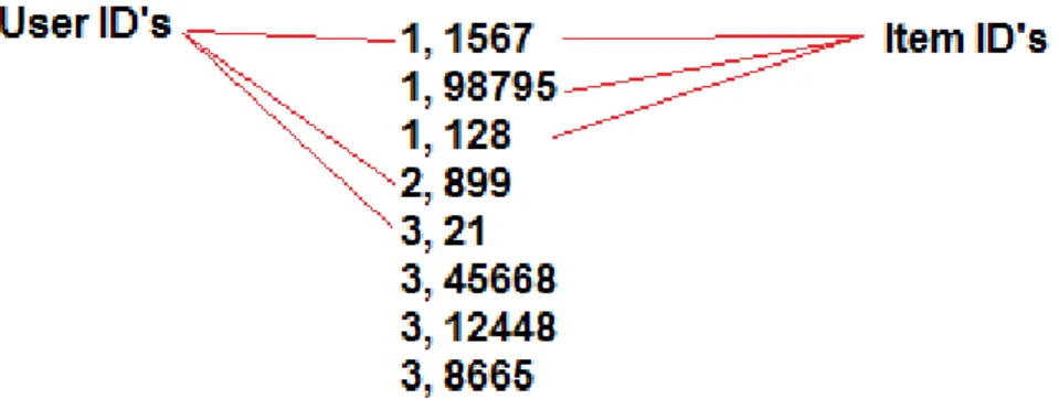
The purchase data we ran our tests on is stored in text files and has the format described in figure 8. In order to enable MyMediaLite to process the data we had to convert them to another format illustrated in figure 9.

(35)

Figure 9: Converted dataset format (the numbers are fictional).

Appart from the converting the format, we also modified the datasets as listed below:

1. Conversion to binary:

The reason for converting the datasets to binary was to evade having to interpret the event of one user having purchased the same item several times. Another approach would have been to calibrate the scoring as was done by Aiolli[4]. In Aiolli’s study the items consist of songs. The number of times a user has listened to a song gives a credible representation for how much the user likes it thus enabling a scoring system resembling ratings. In that aspect, our data differs from that of F. Aiolli’s since several purchases of the same book or fashion item is less probable to represent the user preference than in the case of songs. For example, it is unlikely that the number times a user buy a book is proportional to how much the user likes the book. Calibrating the scoring would also be ineffective in our experiments, as the datasets we used are very close to binary even in their original state.

2. Removal of all users having made less than 2 purchases:

We decided to remove all users having made less than 2 purchases since collaborative filtering requires a certain amount of data in order to produce relevant recommendations. Cold start users can be assumed to benefit more from being shown the top selling items, rather than being shown recommendations based on an inadequate amount of data.

3. Removal of all users having made more than 1000 purchases: We also removed all users having made more than 1000 purchases. Pur-chase records as high as that may distort the results and also indicate

(36)

the user is a company rather than an individual hence not likely to make purchases based on personal preferences.

The modifications to the datasets listed above, as well as splitting them into a training set and a test set resulted in the datasets presented in table 2 and 3 in section 5.1.2.

5.1.2 Splitting the dataset into a training set and a test set

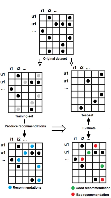
All evaluations we have undertaken have been done offline. The way we have done this is by splitting the datasets into two sets namely a training set and a test set. The training set is the one the algorithms use for learning the patterns of the data in order to produce recommendations. The test set is used for comparing the produced recommendations with the actual purchases originally stored in the test set. There are different ways to split the dataset as well as different split-ratios. A split-ratio of 0,5 means the dataset is split into a training set consisting of 50% and a test set consisting of 50% of the original dataset. Given a split-ratio of 0,5, the MyMediaLite library performs the splitting by randomly removing 50% of the purchases from the original dataset and storing them in the test set, keeping a training set consisting of the remaining 50%. Figure 10 provides an illustration of the training and test-phase.

(37)

Figure 10: Splitting the original dataset and evaluating the recommendations. The green dot represents a recommendation that corresponds to an actual pur-chase in the test set.

(38)

The split-ratio we used was 0.5 as it produced the best results. We did not use the split-ratio property provided by MyMediaLite as it due to its random selection would create different training- and test sets for every test. This would make the results less comparable as the results would also vary to some extent. Instead we used fixed splits thus producing training- and test sets once and use these sets for every test.

For the test set, we kept only users having bought at least 10 items. The reason for not testing on all users were to speed up the evaluation yet still gain results equally comparable among the algorithms. This as well as other measures we took, explained in section 5.1.1 resulted in the datasets presented in table 2 and 3.

Dataset01

Training set Test set Product genre books books Nr of users 304393 19318 Nr of items 175857 70098 Nr of purchases 1219123 203710 Sparsity 99.99772 99.98496

Table 2: Dataset01; training - and test set figures.

Dataset02

Training set Test set Product genre fashion fashion Nr of users 16690 875 Nr of items 4522 2140 Nr of purchases 63086 5962 Sparsity 99.91641 99.6816

Table 3: Dataset02; training - and test set figures.

5.2 Evaluation plan

The evaluation of the results gained from the test we run in our research consist of using the metrics explained in section 2.6 to compare the results of the al-gorithms. In order to produce the values of the evaluation metrics the datasets are split as explained in section 5.1.2.

5.3 Optimizing the parameters

Depending on which algorithm is to be used, there are with some exceptions different parameters to set. The parameters vary depending on which algorithm is used and affect the results in a varying extent. The method we used for

(39)

parameter optimization is golden section search. The golden section search optimization is initiated by setting the following preconditions:

• A lower bound a for the parameter. • A higher bound b for the parameter.

• A value c defines the maximum final gap allowed between the lower pa-rameter value X1, and the higher papa-rameter value X2. The median of X1 one and X2 is the approximation of the optimal value.

The values of the bounds define a range in which the optimal value Xopt for

f (X) is expected to be found, where the function f is the recommender al-gorithm. The optimization process carries through by iteratively moving the bounds towards each other until X1 and X2 has moved close enough to the optimal value as demonstrated in figure 11.

(40)

Figure 11: Golden section search.

In every iteration, new values for X1 and X2 are calculated using the inverse of the golden ratio r as in step 1:

r = −1 + √

5

(41)

Step 1:

X11= b1− r ∗ (b1− a1) (2)

X21= a1+ r ∗ (b1− a1) (3)

Step 2:

In this step, the recommender algorithm f is run using X11 and X21 and the

results returned by f (X11) and f (X21) are compared. We used the F1 metric

explained in 2.6 as it takes both precision and recall into account. Depending on whether f (X11) or f (X21) returns the best results, a new bound a2 or b2 is

set accordingly:

f (X11) < f (X21) => a2= X11∨ f (X11) > f (X21) => b2= X12 (4)

The iterations, consisting of step 1 and 2 continues until |X1n− X2n| < c. At

this final stage, the optimal value for X is set accordingly:

Xopt=

X1n+ X2n

2 (5)

5.3.1 Multi-parameter golden section search

We also had to implement a system for optimizing several parameters. Optimiz-ing them one at a time would most likely not produce the optimal results as the parameters are dependent of each other. In the approach we used, optimizing for example three parameters would carry through accordingly:

1. Run GSS iteration #1 for parameter #1.

5. ...

(42)

Dataset01 Dataset02 BPRMF num iter num factors learn rate bias reg Reg u Reg i Reg j 929 25 0.07663 0 0.0025 0.0025 0.00025 980 68 0.07558 0 0.009098 0.001818 0.003544 WRMF num iter num factors regularization alpha 6 79 0.09002 66.80527 39 39 0.02440 24.3 UserNN similarityFactor dissimilarityFactor 4.00205 0.64105 1.24344 0.46751 UserKnn K Q BinaryCorrelationType 24 7,63971 logLikelyhood 84 4,37712 logLikelihood

Table 4: Parameter values gained from the GSS optimization. Note; the WRMF needs less iterations than the BPRMF since it updates one of the matrices P and QT at a time hence solves the approximation optimization quadraticly.

When observing the optimization process, we noticed that the final param-eter values in some cases did not converge to the optimal values. For some of the algorithms, there were results gained during the optimization process that were better than those gained using the parameters that were supposed to be optimal. A plausible reason for that is that for some parameters p, the f(p)=result function may not be unimodal hence holding more than one maxi-mum. We approached this problem by storing parameters rendering the highest result in every iteration. Should any result during the optimization be higher than that produced using the final parameters, we used the stored parameter values in the final tests. This explains why some of the optimal parameters for the BPRMF optimized on dataset01 kept the default values for parameter Reg u, Reg i, Reg j and bias reg. It must also be mentioned that during the optimization process, we evaluated the recommendations on half of the users from the test set. This in order to decrease the time consumption.

(43)

6 Results

Dataset01

prec@5 recall@5 F1@5 MAP Random 0.00004 0.00002 0.000027 0.00011 Most popular 0.02097 0.01363 0.01652 0.01429 Association rules 0.214 0.15233 0.17797 0.17213 UserNN 0.24675 0.17905 0.20752 0.20058 UserKnn 0,22517 0,16314 0.18920 0,17376 BPRMF 0.0249 0.01426 0.01813 0.0238 WRMF 0.13135 0.09447 0.10990 0.10384

Table 5: The results of all algorithms run on dataset01.

Dataset02

prec@5 recall@5 F1@5 MAP Random 0.00274 0.00197 0.002292 0.00356 Most popular 0.05646 0.04299 0.04881 0.0562 Association rules 0.14537 0.11113 0.12596 0.11362 UserNN 0,14011 0,10806 0.12202 0,11118 UserKnn 0,1248 0,09628 0.10870 0,0915 BPRMF 0.1088 0.08364 0.09457 0.08973 WRMF 0.1232 0.09612 0.10799 0.09821

Table 6: The results of all algorithms run on dataset02.

Tables 5 and 6 present the final results for all the algorithms. In a colored version of this report, the overall best results are colored blue, and the best performing MF algorithm’s results are colored red. Regarding the most popular items algorithm, one must take into account there is no time factor involved as explained in section 4.2. Had the time factor been taken into account, better results would have been expected. The time factor however, plays a big role in all collaborative filtering techniques, although not as significantly as in techniques basing recommendations on top selling items.

For the larger and sparser dataset01, the Association rules and UserNN algorithms performed considerably better than the MF ones, while the difference is much less significant in the smaller and denser dataset02.

(44)

Processing times in hh:mm:ss

Dataset01

Process phase training Prediction and testing total

Most popular 00:00:00 00:23:47 00:23:47 Random 00:00:00 00:27:58 00:27:58 Association rules 00:00:46 00:39:11 00:39:57 UserNN 00:09:34 00:05:00 00:14:34 UserKnn 00:16:05 00:33:12 00:49:17 BPRMF 00:08:14 00:40:45 00:48:59 WRMF 00:35:20 00:27:03 01:02:23 Dataset02 Most popular 00:00:00 00:00:01 00:00:01 Random 00:00:00 00:00:01 00:00:01 Association rules 00:00:01 00:00:02 00:00:03 UserNN 00:00:02 00:00:00 00:00:02 UserKnn 00:00:05 00:00:05 00:00:10 BPRMF 00:00:51 00:00:01 00:00:52 WRMF 00:01:36 00:00:01 00:01:37

Table 7: Processing time consumptions. In a colored version of this report, the overall best results are colored blue, and the best performing MF algorithm’s results are colored red.

As a recommender system’s time consumption is important at least when used online, we also present the time each algorithm needed for training. All tests were run on the same computer. The algorithms vary in the way they distribute the processing to the training- and prediction phase. For example, the UserNN scores all items already in the training phase, hence the low time consumption in the prediction- and testing phase. The difference in size between dataset01 and 02 is considerable, accordingly is the difference in processing time consumptions. The number of purchases is 19 times larger for dataset01 than for dataset02. However, presented as matrices with all empty slots included, the difference in the number of slots is greater than 700 times. These differences in size affect the time consumptions to a large extent.

(45)

7 Discussion

The performance of all the algorithms we tested varies to a large extent depend-ing on which dataset they were tested on. A probable cause of the variation is the difference in sparsity. Even though the differences might not look particu-larly significant at first glance, they must be considered so as for example the training set of dataset02 has almost 37 times as much data in relation to its size than that of dataset01.

In our research, the MF-techniques produced worse results regarding both accuracy and speed on both datasets and for all the metrics we used. The signif-icant differences regard dataset01, where the personalized non-MF algorithms clearly outperformed the MF ones. A plausible reason as to why the personal-ized non-MF algorithms performed better on the larger dataset01 may be that they are not disadvantaged by sparsity itself. As long as there are patterns to learn from, they ignore what in a matrix is known as missing values. The MF algorithms however, need to handle all the missing values. The higher the per-centage of missing values, the more diluted is the data to process. The fact that the MF-techniques performed worse than the other techniques also substantiate our expectations regarding MF-techniques applied on binary or almost binary datasets. Since the datasets we use are almost binary we could not normal-ize the data in order to make it interpretable as explicit. It is probable that MF-techniques are less accurate used on binary data as its numerical values are less nuanced than those of non-binary data. Since MF-techniques depend upon data approximation, they benefit from processing values within a certain range, for example 1-10, which characterizes explicit data which is by definition non-binary. In data approximation, any values outside the range are counteracted as they could not represent the data patterns.

For implicit data and especially binary such, values outside the range of 0-1 is generally not a problem as they indicate a strong or weak confidence of user preference. For this reason it appears association rules and nearest neighbor models are superior for the almost binary datasets we used as these techniques are not constrained to approximate within a certain range.

Among the MF techniques, the best results were produced by the WRMF al-gorithm. The fact that the BPRMF performed considerably worse on dataset01 than dataset02 may be due to the higher sparsity of the former. Since the BPRMF trains on pairs of items, the very large number of items in dataset01 in combination with a high level of sparsity is a probable cause for the poor performance on dataset01. The more items the dataset contains, the less valid

(46)

is the assumption that observed items are preferred over non-observed ones. Since a very large part of the items are unobserved, the data pattern obtained by the pairwise comparison between observed and non-observed items has less significance.

It is also plausible that ALS used by the WRMF is more suitable than SGD used by the BPRMF, when processing very sparse datasets. As explained in section 2.5.2, ALS solves one of the two matrices P and QT at a time, which converges to an unimodal optimization function. Given a matrix has more pos-sible approximation solutions the sparser it is, a multimodal optimization is more likely to converge to a non-optimal solution.

It must also be taken into account that non-MF techniques such as neighbor-hood and association rules can easily be adapted to incremental environments with preserved accuracy performance. This is due to the fact that they can pro-cess one user at a time only taking the data relevant for that particular user into account. There are however techniques for incremental updates also for MF-algorithms. These techniques involve retraining only certain vectors instead of the whole data, thus compromising the accuracy performance. A study of such a technique has been made by Rendle and Schmidt-Thieme[18].

Another important factor at least in online environments is a recommender algorithm’s dependency on parameters. Numerous parameters, strongly influ-encing the results complicate the use in a changing environment as their optimal values may vary along with the data.

(47)

8 Conclusions

We have shown that for various implicit feedback datasets consisting of purchase data, Matrix factorization techniques are inferior to user-based neighborhood techniques and association rules techniques both regarding accuracy and speed. This answers our research question and substantiates our hypothesis, as the results of the Matrix factorization techniques have ranged from being marginally worse to considerably worse than those produced by the other techniques.

We have also presented the UserNN, a variant of a user-based neighborhood algorithm, which have proven to outperform the Matrix factorization algorithms and the UserKnn on the datasets we used, both regarding accuracy and speed. Our results differ from those of [3] in that for the data we experimented on, the choice of algorithm proved to be of substantial importance. The user-based neighborhood algorithm we presented has also proven to produce results com-peting with those of the Association rules model, the top performing algorithm in [3].

8.1 Limitatins of our research

As mentioned in section 6, we have not taken the time factor into account in our research. This implies that the older purchases have gotten the same influence as newer ones. More importantly, we have also to a large extent trained on purchases newer than those we have tried to predict. Another concept we have not researched is user click data, as we only used purchase data in our tests.

As mentioned in section 5.3, we optimized the parameters on partly the same test set as the one we used in the final tests. Another approach would have been to use completely different sets for optimization and final tests. This would have assured the parameters were not optimized for a particular test set. However, given that we during the optimization only evaluated on half the users in the test set, and that we optimized the parameters of all the algorithms using the same procedure, we considered it an appropriate approach for this study.

Regarding the evaluation, due to time constraints we did not use cross vali-dation videlicet we did not run separate tests on parts of the datasets in order to obtain an averaged result. For the same reason we did not use several ran-dom splits in order to run multiple tests on every dataset. However, during the experimental process we unofficially ran multiple test using different splits obtaining results similar to those presented.

(48)

8.2 Future work

Future work will involve researching what we left out in this research namely the the time factor and user click data. As our offline experiments now have shown which techniques perform best on the purchase data provided, the next step is to perform experiments on incremental data involving more factors such as the ones mentioned above. Generally, by studying work related to ours, we have drawn the conclusion that recommender systems running on implicit feedback data in online environments is an area to be further studied in the future.

(49)

References

[1] Congratulations!. (n.d.). Netflix Prize: Home. Retrieved February 14, 2014, from http://www.netflixprize.com

[2] Kantor, P. B., Rokach, L., Ricci, F., and Shapira, B. (2011). Recommender systems handbook. Springer.

[3] Pradel, B., Sean, S., Delporte, J., Gu´erif, S., Rouveirol, C., Usunier, N., ... and Dufau-Joel, F. (2011, August). A case study in a recommender system based on purchase data. In Proceedings of the 17th ACM SIGKDD international conference on Knowledge discovery and data mining (pp. 377-385). ACM.

[4] Aiolli, F. (2013, October). Efficient top-n recommendation for very large scale binary rated datasets. In Proceedings of the 7th ACM conference on Recommender systems (pp. 273-280). ACM.

[5] Hu, Y., Koren, Y., and Volinsky, C. (2008, December). Collaborative filter-ing for implicit feedback datasets. In Data Minfilter-ing, 2008. ICDM’08. Eighth IEEE International Conference on (pp. 263-272). IEEE.

[6] Koren, Y., Bell, R., and Volinsky, C. (2009). Matrix factorization tech-niques for recommender systems. Computer, 42(8), 30-37.

[7] Sarwar, B., Karypis, G., Konstan, J., and Riedl, J. (2000). Application of dimensionality reduction in recommender system-a case study (No. TR-00-043). Minnesota Univ Minneapolis Dept of Computer Science.

[8] Takács, G., Pilászy, I., Németh, B., and Tikk, D. (2008, October). Matrix factorization and neighbor based algorithms for the netflix prize problem. In Proceedings of the 2008 ACM conference on Recommender systems (pp. 267-274). ACM.

[9] Hidasi, B., and Tikk, D. (2012, February). Enhancing matrix factorization through initialization for implicit feedback databases. In Proceedings of the 2nd Workshop on Context-awareness in Retrieval and Recommendation (pp. 2-9). ACM.

[10] Xin, Y., and Steck, H. (2011, October). Multi-value probabilistic matrix factorization for IP-TV recommendations. In Proceedings of the fifth ACM conference on Recommender systems (pp. 221-228). ACM.

[11] Koren, Y. (2010). Collaborative filtering with temporal dynamics. Commu-nications of the ACM, 53(4), 89-97.

Investigating the performance of matrix factorization techniques applied on purchase data for recommendation purposes