Cost-benefit analysis of cycle to work scheme

Master´s thesis • 30 credits

Agricultural/Environmental Economics and Management - Master's Program Degree project/SLU, Department of Economics, 1194 • ISSN 1401-4084

Uppsala, Sweden 2019

Cost-Benefit Analysis of Cycle to Work Scheme

- Implemented in Jönköping Municipality, 2016

Swedish University of Agricultural Sciences Faculty of Natural Resources and Agricultural Sciences Department of Economics

Cost-Benefit Analysis of Cycle to Work Scheme - Implemented in Jönköping Municipality, 2016

Sandra Gradin

Supervisor: Prof. Katarina Elofsson, Swedish University of Agricultural Sciences, Department of Economics; Environmental and Natural Resource Economics

Examiner: Prof. Rob Hart, Department of Economics; Environmental and Natural Resource Economics

Credits: 30 hec Level: A2E

Course title: Master Thesis in Economics Course code: EX0811

Programme/Education: Agricultural/Environmental Economics and Management - Environmental Economics and Management

Faculty: Faculty of Natural Resources and Agricultural Sciences Course coordinating department: Department of Economics Place of publication: Uppsala

Year of publication: 2019

Name of Series: Degree project/SLU, Department of Economics No: 1194

ISSN 1401-4084

Online publication: http://stud.epsilon.slu.se

Swedish University of Agricultural Sciences Faculty of Natural Resources and Agricultural Sciences Department of Economics

iii

Abstract

In a response to negative externalities such as GHG emission, health costs, infrastructural costs, noise and air pollution etc. caused by motorised transportation international

organizations and governments have started promoting shifts towards active transportation such as walking and cycling. This study use a CBA-framework to evaluate a cycle to work- scheme implemented in Jönköping municipality in 2016. The scheme allowed all

municipality employees to lease bicycles or e-bikes for a three year period and pay for them through a salary sacrificing arrangements, after the three year were over the participants could either buy the vehicle at market value or return it free of charge. Eleven parameters were included in the CBA, the internalisation through taxation/fees of some of the effect for some parameters were taken into consideration as well as the shorter Swedish bicycle season (31 weeks on average). The result indicate a benefit-cost ratio of 6.21:1, meaning that C2W scheme is a cost efficient method of increasing AT usage.

vi Acknowledgements

Thanks to everyone who helped in completion of this thesis, employees at Jönköping Municipality who helped supply me with information. And a special thanks to Rikard.

vii Abbreviations

AT- Active transport GHG - Greenhouse gas

GWP- Global warming potential LCA - Life cycle analysis

MCF/MCPF - Marginal costs of public funds MEB - Marginal excess burden of taxes MET- Metabolic equivalent of task NCD - Non communicative disease NVV - Naturvårdsverket

PA - Physical activity

VSL - Value of statistical life VTTS - Value of travel time saved WHO - World health organization

viii

Table of content

1.1 Aim and delimitations ... 3

1.2 Structure ... 3

2. Background ... 4

3. Literature Review ... 7

4. Method ... 10

4.1 CBA: Introduction and Outline ... 10

4.2 CBA: Criticism and Limitations ... 11

5. Case Study Description ... 14

5.1 Background ... 14

5.2 C2W Scheme ... 14

5.3 Counterfactual ... 16

5.4 Data collection ... 18

5.4.1 Survey mode ... 19

6. Costs and Benefits - Effects and Cost Calculations ... 21

6.1 Health ... 22

6.1.1 Physical activity ... 22

6.1.2 Noise pollution ... 24

6.1.3 Local and Regional Air Pollution ... 26

6.1.4 Accidents... 30

6.2 Travel time ... 33

6.3 Parking ... 34

6.4 Vehicle Purchase and Operation ... 36

6.5 Climate change ... 38 6.4.1 Pricing CO2 emission ... 43 6.6 Implementation Costs ... 44 6.7 Absenteeism ... 44 6.8 Infrastructure ... 45 6.9 Discount rate ... 46 6.10 Internalisation ... 47 7. Result ... 49

7.1 Cost and Benefits - Applied to the Case Study ... 49

ix

7.1.3 Travel Time ... 52

7.1.4 Parking ... 53

7.1.5 Vehicle Purchase and Operation ... 53

7.1.6 Climate Change ... 54 7.1.7 Implementation Costs ... 54 7.1.8 Absenteeism ... 54 7.1.9 Infrastructure ... 55 8. Sensitivty analysis 56 9. Discussion... 60 10. Conclusion ... 64

Appendix A: Summary of Studies Included ... 65

Appendix B: Bicycles ... 68

Appendix C: Parameters excluded ... 69

Appendix D: HEAT ... 70

Appendix E: Survey sheet ... 71

Appendix F: Internalisation of cost from vehicles that run on ethanol fuel 72

x List of figures

Figure 1: Economic sectors and their CO2 emission.

Figure 2: Daily total distance cycled in Sweden each day, 1995-2014. Figure 3: Automobiles in Sweden, 1923-2014.

Figure 4: BCR of included studies.

Figure 5: The percentage of users for varying transportation modes during the weekday and weekend in 2009 and 2014.

Figure 6: The average amount of passing passengers in nine bicycle measuring points in Jönköping city during the time period 2012-2017.

Figure 7: C2W participants answers to the question “were you planning on purchasing a bicycle/e-bike independently of the C2W scheme?”.

Figure 8: The age dispersion of the participants in the C2W scheme. Figure 9 : Map of Sweden with five ventilation zones. circle. Figure 10: Emission from automobiles during their entire

Figure 11: NPV for each year within the time frame, using varying discount rates.

List of tables

Table 1: Summary of the survey given to the participants in the C2W scheme.

Table 2: All parameters included in the CBA, the methodology to quantify them and what data was used.

Table 3: Summary of marginal cost/benefit from increased PA for all transportation modes.

Table 4: Summary of all marginal costs due to noise pollution. Table 5. The ventilation zones and belonging ventilation factor. Table 6: The values of the local effects of air pollution.

Table 7: The values of the regional effect of air pollution emission. Table 8: Summary of marginal costs for local and regional air pollution.

Table 9: Emission factors for nitrogen oxide (NOx), non-methane volatile organic compounds (NMVOC), sulphur dioxide (SO2) and particles from road/tire friction (PMm) for automobiles.

Table 10: Emission factors for nitrogen oxide (NOx), volatile organic compounds (NMVOC), non-methane sulphur dioxide (SO2) particles from road/tire friction (PMm) for a bus which runs on biofuel.

Table 11: Summary of marginal cost for accidents for all transportation modes. Table 12: Summary of marginal travel time costs.

Table 13: Summary of marginal parking cost.

Table 14: Purchase and operating costs for all transportation modes. Table 15: The marginal cost for climate change for all transportation modes.

Table 16: Summary of marginal infrastructural costs for all transportation modes. For automobiles and buses the price during warmer conditions is first followed by the price in winter conditions.

Table 17: Summary of all cost and benefits estimated in this study

Table 18: Summary of all yearly costs for noise pollution, all transportation modes.

Table 19: Summary of all yearly costs for local and regional air pollution, all transportation modes. Table 20: Summary of yearly cost and benefits due to change in accidents.

Table 21: Summary of all yearly costs due to change in travel time Table 22: Summary of yearly parking costs for all transportation modes.

Table 23: Summary of all the costs and benefits from change in vehicle purchase and operation. Table 24: Summary of cost for climate change (emission of CO2-eq) for all transportation modes

Table 25: Summary of infrastructural cost for all transportation modes.

Table 26: All cost and benefit estimates for one bicycle season using three different discount rates: 1%, 3.5% and 6%.

Table 27: Benefit from PA with different discount rates and with different internalisations degrees due to substitution (0, 0.25 and 0.5).

Table 28: NPV with varying discount rates and different internalisation degrees due to substitution (0, 0.25, 0.5). Table 29: The costs, benefits and NVP for only with internalisation and seasonal usage (31 weeks)

1

1. Introduction

The accelerating pace at which the planet is heating has become an ever-increasing global threat (NASA, 2016). Scientists attribute the worrisome development to the increasing emission of greenhouse gases (GHG). Due to anthropological activity producing an excess of GHG, primarily during the last decade, the atmospheric concentration of carbon dioxide, methane and nitrous oxide are unprecedented in the last 800,000 years (IPCC, 2014). The impact on people and ecosystems are immense; changes in hydrological systems which affect water resources negatively in terms of both quantity and quality, reductions in crop yields, ocean acidification and extreme weather including; droughts, floods, hurricanes and wildfires are some of the effects that are to some extent already taking place but without a change in GHG emissions are expected to worsen (IPCC, 2014). A continuation of GHG emissions at similar rate will have a severe and irreversible effect on the way we live our lives today as well as the ability for future generations to live theirs. To avoid worsening climate effects and capping the global average increase in temperature at 2 degrees, the International Panel on Climate Change (IPCC) advises a decrease in GHG emissions with 40-70% by 2050.

Figure 1: The world's economic sectors; electricity and heat production, agriculture, forestry and other land use (AFOLU), buildings, transport, industry and other; and their respective percentage of CO2 emission. (IPCC, 2014)

The world's economic activity that is responsible for almost all CO2 emission can be divided into six primary sectors seen in figure 1 above. Despite some sectors emitting more than others a change is needed in all to accomplish the ambitious goals of a CO2 concentration not higher than 450-500 ppm, at which it is likely that the temperature does not rise more than 2 degrees above pre-industrial levels. One sector not expected to meet the demand of change is the transport sector. Instead, due to the growing numbers of passenger and freight transportation the emissions of GHGs is estimated to increase by 50% by 2030 and more than 80% by 2050 despite the potential of GHG decrease in the sector being deemed as high (IEA, 2009; IPCC, 2014). Many influential organizations, the World Bank, UN, WHO and the EU have recognized

25%

24% 6,40%

14% 21%

9,60% _{Electricity and heat production}

AFOLU Buildings Transport Industry

2

the importance of emission decrease in the transport sector and promote various methods of decrease emission and, to the extent possible, create a modal shift from motorised transportation, towards more sustainable active transport (AT) such as cycling and walking (Dill et al 2009; Cavill et al 2006; WHO, 2002; European commission, 2018).

In Sweden, the transport industry (primarily passenger vehicles) produced one third of all GHG emissions, but unlike globally, the emission are slowly decreasing (NVV, 2017). The decrease is not due to a reduction in numbers of automobiles or average mileage driven, which both have increased but rather substitution for more fuel-efficient vehicles. Nonetheless, to be in line with the set environmental goals the transition is not fast enough and the Swedish government much like other organizations maintains that a decrease in passenger cars as well as freight transportation is necessary. This ambition is included in the government's environmental plan, where the importance of decreased motorised transportation is highlighted in 4 out of 16 environmental goals (Miljömål, 2018).

AT had been suggested as part of the solution to the increasing GHG emissions from the transportation sector, but it has also been previewed as part of the solution to the problems that the increasingly sedentary modern lifestyle cause. The recommended amount of weekly moderately intense aerobic physical activity is 150 min, but in 2016, 28% of the world population (1.4 billion) were below this and estimated to be “at risk of developing or exacerbating diseases linked to inactivity” (WHO, 2010; Guthold et al, 2018). In Sweden the numbers are slightly more encouraging but still 21.5% of all men and 24.7% of all women do not move sufficiently enough to avoid negative health effects (Guthold et al, 2018). Physical inactivity is now one of the leading causes behind an increase of a variety of non-transferable diseases (NCDs) such as cardiovascular diseases, diabetes, colon cancer, high blood pressure, osteoporosis, lipid disorders, depression and anxiety (WHO 2002; Hallal et al, 2012; Thorp et al, 2011). The cost for the increase in NCD is not only in human suffering but the social cost for medical assistance is considerable. A large study including 142 countries conservatively estimated that in 2013 the worldwide health care system cost for physical inactivity was $53.8 billion as well as related deaths contributed to $13.7 billion in productivity losses and 13.4 billion disability adjusted life years (DALY) (Ding et al, 2016).

Increased AT has been proposed as part of the solution to the negative externalities caused in part by motorised transportation. But in addition to having impacts on the climate and activity levels motorised transportation cause additional externalities for which the first hand consumer does not bare full cost. Externalities such as congestion, noise and other environmental unfriendly pollutants, space consumption, accident costs and road wear. As a result increased AT is recommended from the absolute top political organs down to local municipality levels. The measures to encourage AT and discourage motoring comes in many forms with varying results, but since the governmental resources are limited the cost needs to be carefully measured against the benefits.

3 1.1 Aim and delimitations

In an attempt to address the negative externalities caused by passenger transportation Swedish governmental agencies at all levels have started to implement measures to increase active transportation modes. One example of this is the cycle to work-scheme (C2W) implemented by Jönköping municipality in 2016. The scheme allows municipality employees to lease bicycles or e-bikes for a three year period and pay for them through a salary sacrificing arrangement. After the three years the participants can either buy the vehicle at the current market price or return it. This study aims to calculate all private as well as social costs and benefits of the implementation in an attempt to determine if it is economically justified. There is a lack of such evaluations, internationally but particularly within a Swedish context, given winter conditions and internalisation of externalities through taxation. It also, unlike any other study found, includes e-bikes (electric bicycles) which have been popular for a long period of time in other parts of the world but are a rather new transportation mode in Sweden and therefore somewhat lacks evaluation.

The study is limited to a smaller sized city, Swedish seasonal cycling conditions and Swedish tax policy. It is also limited to a 12 year long period (2016-2024) based on the life expectancy of a bicycle. Since the evaluation is medias res, meaning that the evaluation takes place before completion of the implementation, the full effect is not calculated. The result presented here is only a part of the total outcome from the complete implementation, and should be treated as such.

1.2 Structure

The thesis consists of ten sections in total; section two is meant to give the reader a deeper background of the history of transportation vehicles, travel behaviour and political approach. In section three an overview of the previous literature on this is presented. In section four the CBA framework is presented and criticism and limitations with the framework is discussed. Section five is where the reader will gain information about the case study in question, as well as the counterfactual and data collection. In section six, the parameters included in the CBA are presented; how they are measured and to some extent the limitations of these measuring methods. The parameters from section six are then applied to the case study in section seven, where the costs and benefits from the implementation are presented. Section eight and nine tests and discusses the findings from previous section and lastly the findings are concluded in section ten.

4

2. Background

Historically, the bicycle have had a longer time to make an impact on human life than the automobile. When the first blueprint for the bicycle originated is still a matter of discussion but the first documented bicycle then known as a “draisine” was constructed by Baron Karl von Drais in 1817 (Herlihy, 2006). Since then it has had many different names and designs, but it was not until 1885 when the first “safety bicycle” was produced the bicycle became a commercial hit. The vehicle was cheap, light weight, safe and offered extended opportunities of mobility. Only a few years later it was the most popular mode of transportation in Europe and America (Herlihy, 2006). The bicycle remained its popularity in Europe during the first part of the 20th century whilst in America the automobile made its debut and flooded the market (Herlihy, 2006). In Sweden bicycling remained popular until the 1950s when the automobile took over, but after 20 years of low demand, in the 1970s the bicycle return to the public eye and bicycling started increasing again (Miljöbarometer, 2018). During the last 20 years bicycling in Sweden had decreased but this trend has stagnated the last couple of years and its popularity remain rather constant. (Trafikanalys, 2015; Regeringskansliet, 2017)

Figure 2: Total distance cycled in Sweden each day (1000 km), 1995-2014 (Trafikanalys, 2015)

The e-bike has an equally long history in theory but since the design demands more advanced technology it was for a long time limited by the heavy electrically driven wheels and low range battery and not until the invention of lighter batteries in the 1990s it became a commercially sold item (Electricbikereport, 2016). In Sweden e-bikes had a slow start and it was not until 2015 that sales grew to significant size, and by 2018, 12% of the total market of bicycles was e-bikes and 38% of all Swedish individuals could see themselves purchasing one (Svensk cykling, 2018). In modern times however, neither the bicycle or the e-bike can compare to the impact of the automobile; in 2015 there were almost a billion automobiles in operation

5

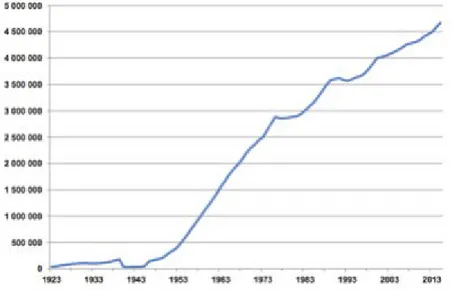
worldwide (Statista, 2018). In Sweden the number of automobiles have steadily increased since 1943 and in 2017 there were 4.8 million automobiles in total (SCB, 2018).

Figure 3: automobiles in Sweden (1923-2014) (SCB, 2018)

The field of travel behavior offer several economical, psychological and sociological suggestions as to what the driving forces behind choice of transportation mode are. On a macroeconomic scale the rate of increase in driving shows correlation with GDP growth as well as a decrease with economic recessions and increased fuel prices, indicating that economics is highly influential on our travelling habits (ACEA, 2018). In addition there is extensive research suggesting various psychological reasons for our travel choices, such as; pre-existing attitudes, “perceived barriers to behavior”, habits or affective motives (Anable, 2004). There is also evidence that we have an irrational bias towards automobiles and that they exhibit “travel mode stickiness” meaning that once an individual has chosen automobiles as a first choice they are inclined to change this decision (Innocenti et al, 2013). The underlying individual factors for choice of transportation mode are many, but there are also other practical reasons why someone would choose one transportation mode over another such as large variation in altitude, the possibility of combining transportation modes, well-functioning and maintained cycling infrastructure.

Historically, most of the political focus when encouraging shifts in transportation modes has been on just harder measures such as infrastructural improvements, prohibitions or economic tools. This can still be seen when reviewing the national Swedish cycling strategy as well as Jönköpings municipalities bicycle plans in which the majority of focus and funding are on harder measures (Regeringskansliet, 2017; Jönköping kommun 2016/2017). This focus is not wrong per say since, as mentioned, good and safe infrastructure is important when individuals decide on transportation mode and the majority of literature that examine these kinds of harder measures generally indicate cost efficiency. However, these measures may not on their own be

6

effective enough to promote travel mode shifts and some may be problematic to implement due to public opinion or political infeasibility (Bamberg et al, 2011). This has paved the way for an increase in soft transportation measures (mobility management), meaning “techniques of information dissemination and persuasion to influence car users to voluntarily switch to sustainable travel modes” (Bamberg, 2011). Most research indicates that soft measures complement harder ones and they have grown in popularity, especially at municipality level (Dill et al, 2010; Epom, 2018).

7

3. Literature Review

There is a substantial amount of literature evaluating policies aimed to increase AT, the majority is focused on infrastructural changes but there are those who evaluate other actual or theoretical changes in transportation modes. However there is not much literature that evaluates C2W schemes specifically and only three studies were found. Clarke et al (2014) have written the only CBA of a C2W scheme in which they investigate the C2W scheme implemented in Scotland. They consider an extensive amount of parameters including the forgone tax cost for the government, but they do not include travel time which generally is one of the bigger cost parameters for cyclist. The results are in line with similar research on bicycle investments with a benefit-cost ratio (BCR) of 3.51 and 2.55 (depending on varying definitions of the forgone tax for the government).

The second evaluation of a C2W scheme done by Green et al (2016) is not a CBA but there is comparisons of the health cost and benefits from increased physical activity (PA). They look at the increased amount of PA for 13,000 scheme users in England and Wales and concluded that 65% of these users rapport a 30 min daily increase of PA. They then (conservatively) estimate that if only 5% of the 180,000 total users would increase their PA by 30 min daily the social benefit from reduced absenteeism and increased health levels would be £72 million yearly, and the BCR would be 2.

They then go on and assume if these results are moderately applied to the total amount of users; meaning if only 5% of the 180,000 total users would increase their PA by 30 min daily the social benefit from reduced absence and increased health would be £72 million yearly, and the BCR would be 2. They do not question any possible substitution between AT and other PA. The last evaluation of a C2W scheme is by Caulfield & Leahy (2011) who looked at the users of the Irish tax relief scheme introduced in 2009 which is similar to C2W scheme in Jönköping. They conclude that 95% were satisfied with the scheme (73% very satisfied), that the individuals who did not own a bicycle prior were encouraged to do so because of the scheme and that this could result in a “substantial modal shift toward cycling” (Caulfield & Leachy, 2011).

In addition to these evaluations of C2W schemes there are two other categories of literature that are relevant to this thesis. Firstly there is literature not concerned with C2W schemes specifically but rather evaluations of infrastructural changes or other (sometimes hypothetical) implementations. These studies were still considered relevant due to data/methodological similarities (an overview of all studies included can be seen in appendix A). The inclusion of studies was primary based on similar definitions and inclusion of parameters (the difficulty with this will be discussed later) as well as the presence of a BCR (seen in figure 4) for comparability purposes. Secondly, since the means of transportation many times is a public good and handled at least to some extent by the government there is a vast amount of “grey literature” produced by governmental agencies, that is not published nor peer reviewed. They

8

seldom conduct their own empirical research but rather gather expert opinion and recent evidence within the field to form recommendations and frameworks for national transport evaluation. In this thesis the primary sources of literature in this category is the Swedish Transportation Agency (Trafikverket) which has a framework for evaluating implemented transportation policies within the Swedish context (Trafikverket, 2018; Trafikanalys, 2017). Their recommendations will be loosely followed in section 6.

Figure 4: BCR of included studies.

The majority of studies evaluating infrastructural changes use a CBA framework (or similar method) which has become the most common and powerful tool to evaluate planning and policy efforts (Li & Ardeshir, 2014). There is close to a consensus about investments in AT being a cost efficient alternative, meaning that the BCR>1 (see figure 4). The only noticeable exception to this, is the study by Foltýnová & Kohlová (2002) in which the BCR was -0.97. This was one of two studies that considered demand for the bicycle investment (PWC also included a demand forecast), and in which only 0.2% of the city’s residents used bicycles which could be the reason for the negative BCR. Even though a clear majority of all studies indicate similar results, there is great variation on how these conclusions are reached. The EU recognized this problem and in 2005 they started a project called HEATCO (developing harmonized European approaches for transport costing and project assessment) which after overseeing existing “national transport infrastructure project assessment” concluded that despite most nations having national guidelines they “differed widely in terms of their methodology, level of detail and indicators” along with “differences in assumptions between

countries in terms of the economic valuation of impacts” (IER, 2006). The project, which was

finished in 2006, set out to create “harmonized guidelines for project assessment and transport

-10 0 10 20 30 40 50 60 70 AE CO M (2010) Ba uf el dt e l a t ( 2017) (S 1) Ba uf el dt e t a l ( 2017) (S 2) Bu is ( 2000) (S 1) Bu is ( 2000) (S 2) Bu is ( 2000) (S 3) Bu is ( 2000) (S 4) Bö rje ss on & E lia ss on (2012) Ch ap m an e t a l ( 2018) Cl ar ke e t a l ( 2014) (S 1) Cl ar ke e t a l ( 2014) (S 2) Co pe e t a l ( 2010) * De pt o f tr an sp ort at io n ( 20 07 )… De pt o f tr an sp ort at io n ( 20 07 )… De pt o f tr an sp ort at io n ( 20 07 )… Li & F ag hr i ( 2014) Fo ltýn ov á & Ko hl ov á ( 2002) Gr ee n e t a l ( 20 16 ) Go ts ch i ( 2011) (S 1) Go ts ch i ( 2011) (S 2) Go ts ch i ( 2011) (3) M ac m ill ia n ( 2014) (S 1) M ac m ill ia n ( 2014) (S 2) M ac m ill ia n ( 2014) (S 3) M ac m ill ia n ( 2014) (S 4) PW C ( 2009) Sæl en sm in de (2004) (S 1) Sæl en sm in de (2004) (S 2) Sæl en sm in de (2004) (S 3) SQ W (2007) (S 1) SQ W (2007) (S 2) SQ W (2007) (S 3) SQ W (2007) (S 4)

9

costing at EU level”, but despite this many independent researchers do not apply to the framework, thus the problem with comparability remain.

The problem does not only exist with the definition or estimation, but also, with the somewhat arbitrary decision making- process in the inclusion/exclusion of parameters. This is exemplified in appendix A where there is no identical combination of parameters in any of the included studies. These issues are not helped by the (in many studies) lack of transparency regarding the thought process behind the parameters both included and excluded. Due to these methodological differences comparisons between studies needs to be made with great caution.

10

4. Method

4.1 CBA: Introduction and Outline

The CBA framework entails assessing, calculation and comparing all benefits and costs of a policy in an attempt to make a well informed decision about whether to implement a policy or not. The aim is to identify the most cost efficient alternative and the framework has become a widely used tool in planning and policy making, especially within transportation planning (Mingxin & Faghri, 2014). Whether a project should be implemented or not is primarily based on the cost-benefit ratio (BCR) meaning, the ratio of the benefits from a policy relative to its costs. The idea is simple: if the BCR is larger than 1 the policy should, on economic grounds at least, be implemented since it would increase the social welfare, and if it is smaller than 1 it should not be implemented since the resources could be used more efficiently elsewhere (Gordon, 2017). The objective with a CBA is to include costs/benefits that affect the entire society rather than just the individual and it is therefore sometimes also referred to as a social cost and benefit-analysis. There are different time perspectives that can be adopted within a CBA-framework, the analysis can either be (1) ex-ante; before the implementation of a policy or (2) post-ante after the implementation of a policy. These are the most commonly used time-frames, but there is also a third time frame alternative;(3) medias res, meaning the evaluation takes place at the same time as an ongoing policy (Boardman et al, 1994). The steps in all time variant versions of the CBA are similar, but there can be some variation as too what the steps entail or in which order to perform them. According to (Hanley & Spash, 1993) the essential steps are:

(1) Defining the project. What is the project and what is its counterfactual to be compared with? The counterfactual can be some other policy with the same purpose or it can be the most common, status-quo, meaning that no other policy is implemented. Other questions are what reallocation of resources is being proposed and who have standings in either the project or in the counterfactual?

(2) Identifying impacts which are economically relevant. Environmental impacts count if 1) they change the wellbeing of one individual and/or 2) change the level or quality of output of some positively valued commodity.

(3) Physically quantification of relevant impacts. Determining the physical quantities of the effects of the implementation within the time-frame.

(4) Calculating a monetary valuation of relevant impacts. To be able to measure and compare things they must be quantified in the same units; dollars (or some other currency). This is not to say that money is all that matters but for there to be comparison some attributed value has to be concluded and despite its complicated nature, price does carry valuable information (Hanley and Spash, 1993). The CBA analysts must then do three things to address this 1)

11

predict prices of value flows extending into the future 2) correct market prices where necessary 3) calculate prices (relative values in common units) where none exists. Point 1) entails a necessity of calculating using real values, since nominal values does not give an accurate representation of values in real time. Point 2) and 3) entails adjusting and calculating alternative market prices to estimate what is known as a shadow price. This is often done with unconventional pricing methods, which will be discussed in section 4.2.

(5) Discounting costs and benefit flows. When values for the costs and benefits have been determined it is necessary to express them in present value (PV). Meaning that since humans have a time preference, ten dollars are worth more for us today when it is spendable than in one year from today, and therefore future costs or benefit need to be discounted to PV. The need for this is either due to human impatience to consume or the possibility to invest today and yield greater economic winnings in the future. To accurately calculate future costs and benefits in present value a present value-formula is used:

(1) (C) = future value, i = interest rate, n= time period (most often years)

(6) Net present value test (NPV). The determinant of whether an implementation or a policy is social beneficial is whether the sum of the discounted benefits is greater the sum of the discounted costs.

4.2 CBA: Criticism and Limitations

The straightforwardness and intelligibility of CBA is undoubtedly one of its strengths, in practice however, the situation is more complicated and this strength can become a weakness. The criticism of CBA’s can be divided into two major groups: criticism of the framework and theoretical ground on which it is based and criticism of the practical usage of it. Framework and theoretical ground

The need to monetize parameters, primarily softer parameters, have been ongoing subject of criticism. There are moral dilemmas that stem from giving monetary value to the parameters in a CBA. Firstly some question whether it is at all right to do so with living things such as the environment or even human beings and secondly, how do we value future generations wellbeing or intergenerational fairness (what discount factor should be used?). (Ackerman & Heinzerling 2002, Frank 2007). Gerrard exemplifies the problematic nature of this by stating

12

“if a human life is considered to be worth $8 million, and a ten percent discount rate is chosen, then the present value of saving a life one hundred years from now is only $581. Neither I nor anyone else use this kind of argument” (Gerrard, 1998).

Furthermore the CBA framework rests upon a utilitarian theory (or other similar consequentialist ethical theory) and critics mean that this in itself comes with a ethical dilemma; sometimes the alternative that maximizes the utility is not necessarily the best one for all (Frank, 2007). This criticism entails that the CBA is inherently unjust and that this causes a distributional problem, for example since it gives equal weight to a project for the rich as well as a project for the poor it does not take proper account of the effects of policies, concerning the distribution of burdens and benefits in society (Copp, 1987). Copp also argues that by measuring benefits and costs only in dollars there is implicitly greater significance given to the welfare of the richer members of society. Lastly one other concern with the framework has been raised primarily due to new findings in the field of behavioral economics and addresses that CBA’s are performed assuming an individual application of rational choice theory, but some argue that human decision-making is in itself a social, and not only an individual process (Parks & Gowdy, 2013).

Practical usage

Like mentioned previously, since many frequently used parameters in CBAs lack market value other methods to estimate shadow prices have to be used. These methods primarily consists of surveying methods and drawing inference from market behavior; both methods are associated with some difficulty and uncertainty. The problems with surveys are that they often consists of contingent valuation (CV) which can be problematic for a number of reasons. Firstly the monetary value of the outcome asked to be appraised often exceeds the individual's total wealth, secondly the answers to CV surveys are often very sensitive to how the questions are formulated and thirdly there are problems with loss aversion; meaning that individuals are much more likely to “prevent a harmful effect than to undo a harmful effect that has already occurred” (Frank, 2007). Another way of expressing this is that there are differences between the willingness-to-pay (WTP) and the willingness-to-accept (WTA) that are problematic when interpreting the result of a CV survey.

Making estimates from market behavior using hedonic pricing methods (or indirect economic pricing) is also affiliated with high levels of uncertainty due to incomplete information, immobility and other imperfections (Frank, 2007). Varying hedonic pricing methods are applied in the housing and labor market as well as the market for environmental services. Different parameters are faced with varying estimation problems and the concerns regarding monetary evaluation of parameters (ecological and others) are summarized as follows: (1) does not capture ecological sustainability and distributional fairness (2) possible value incommensurability (impossible to find a monetary value) (3) prices are a result of historical context and reflect historical and existing power structures (4) marginal values should not be

13

confused with total values (5) marginal values should only be used when ecosystems are fairly intact and functioning normally (6) tends to leave policy makers without responsibility (Røpke S, 2005; Howarth & Farber 2002; Parks & Gowdy, 2012; Limburg et at 2002).

One last concern, which has been discussed previously is the human decision making process when including or excluding parameters. As can be seen in appendix A in this thesis and in many other reviews on the topic there is great variation on what parameters are included, which obviously has an effect on the outcome. Some justify the exclusion of some parameters due to the uncertainty mentioned above, while others argue that the same parameters contribute enough information to be worth including. Either way the decision is somewhat arbitrary, possible making the outcome such as well, this will be discussed further in section 9.

14

5. Case Study Description

5.1 Background

Jönköping municipality has a long history of softer transportation measures such as bicycling courses for newly arrived female immigrant, free courses in bicycle mechanics and variety of information campaigns aimed at informing about the benefits with AT (Jönköping kommun, 2017; Temp, 2008). In 2016 they reformulated the 10 year old bicycle-program and highlighted the importance of safe and efficient bicycle investments as a way to increase AT. It underlines that all more environmentally friendly transportation such as bicycle, walking and public transportation should be prioritised over motorised transportation (an opinion also shared by 58% of the residents) (Jönköping kommun, 2017).

When Trafikanalys reviewed how much resources were assigned to bicycle measures in all counties, Jönköping county was the only county that had not separated the resources assigned for bicycles from the resources assigned to public transportation, the total amount for both is 120 million (Trafikanalys, 2014). The budgeted amount on municipality level is 17 million annually, but in 2016 the spending exceeded this which was taken from the budget planned for 2017. For 2018 the budget was increased to 21 million. This spending are accompanied by ambitious goals; the municipality aims to increase cycling during weekdays by 25% between 2014 and 2019. And since the majority of all trips are made with automobiles, ⅓ of all journeys in the municipality are shorter than 3 km and ½ shorter than 5 km the goal is to replace shorter automobiles journeys with bicycle or e-bikes (Jönköping kommun, 2017).

5.2 C2W Scheme

The C2W scheme was implemented in Jönköping municipality in May of 2016 and is planned to continue till spring 2019; with several occasions (at least 2 each year) for municipality employees to lease vehicles. One demand from the municipality was that it should be (or close to) cost neutral and therefore the implementation was carried out via the company Ecochange which has provided both private and governmental/municipal employees with a variation of employee benefits. The scheme gave everyone the almost 10,000 employees at the municipality the opportunity to lease bicycle/e-bikes (maximum 2 vehicles per person) over a 3 year period and when the time period expired they were offered to either buy their vehicle at current market price or return it to Ecochange. During the time frame of this thesis, three leasing opportunities passed, in which a total of 2346 vehicles were leased, by 2012 individuals. Out of which 954 were bicycles and 1392 e-bikes, this means that some individuals leased more than one vehicle, either for themselves or for someone else. According to employees at Ecochange, 90% of all participants purchased their vehicle at the end of the leasing period. There were several different bicycles and e-bikes available, ranging from tricycles and foldable e-bikes to city and race bicycles (an overview of the models can be seen in appendix B). The payment was

15

processed by a gross wage deduction with the total price for the individual leasing was dependent on two things; 1) price of vehicle chosen 2) the individual's marginal tax. In Sweden there is an increase in marginal tax depending on income level, if an individual earns more than $49,880 each year the margin income increases from 33% to 56%

The municipality handled the initial marketing and information about the scheme to the employees. The communication was done via their intranet and through email, meaning that the administrative costs were very low. The local media also covered the initiative in several news outlets which probably contributed to the high participation amongst the employees (around 20%). The municipality did not do any of the practical work, moving or distributing the vehicles, the entire rental service itself was carried out by Ecochange. Location

The location of the C2W scheme is the city of Jönköping which is located in the middle part of Sweden (see figure 6). The city is the 10th largest city in Sweden and inhabit 137,481 people (Jönköping kommun, 2018). The city is located next to Sweden's second largest lake (Vättern) which cause large differences in altitude, primarily when entering/exiting the central area of the city.

Project time

The time limit of this project is 12 years, this time limit is based on the life expectancy of a bicycle. Obviously the lifespan of a vehicle is dependent on many things, how it is operated, maintenance, original quality etc. Trafikverket use the age estimate 10-16 years depending on the type of bicycle (Trafikverket, 2018). The life expectancy of the battery on e-bikes is shorter, but can be replaced. It should be noted that this thesis does not evaluate the entire implementation made in Jönköping. The time frame for evaluation of this implementation is medias res, meaning that when this evaluation is performed the scheme is still not completed. This means that the monetary outcome of this thesis is smaller than the outcome for the entire scheme. It is likely to assume that given the same municipality employees the effect is decreasing since fewer and fewer lease vehicles. But still, the outcome in this thesis should be noted as only part of the total outcome of the entire implementation.

Standings

The most obvious people who have standing in the scheme are the participants who’s wellbeing change through joining the scheme (consumers). The people who supply the scheme also have standing (producers). On a larger scale, other residents in the municipality (or people who are passing through) who are otherwise affected by some of the local externalities from automobiles such as noise pollution and local/regional air pollution also have a standing (third

16

party). And on the largest scale, everyone who is affected by climate change have a standing, since CO2 emission is a global problem.

5.3 Counterfactual

When considering the counterfactual, the question that needs answering is; what would have happened if no policy was implemented given ceteris paribus? In this case, how would the bicycling amongst the municipality employees changed had the C2W-scheme not been implemented? To answer this, observing the bicycle trend in Jönköping, prior to the scheme, could offer some insight.

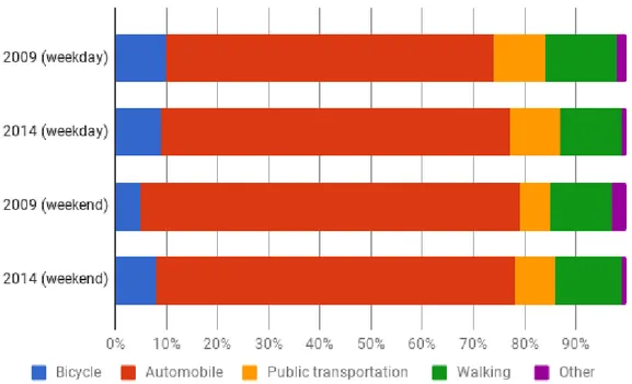
There has been transportation data collected in two studies that charted the travel habits of individuals living in Jönköping. Both studies were conducted in the same form with a postal survey being sent to 7000 people, for which they had similar respond rate of 47% and 43% for 2009 and 2014 respectively (Billsjö et al, 2014). As seen in figure 5, the travel habits during the weekdays remain fairly constant between the years with the most notable difference being a 4% increase in driving. The same is true for the weekends, with the exception of a 4% increase in cycling and a 3% increase in public transportation. The difference between weekday and weekend are similar for both years in that there is an increase in driving (10% in 2009 and 2% in 2014) while there is a decrease in all other transportation (with the exception of walking which in 2014 had a 1% increase).

Figure 5: The percentage of users for varying transportation modes during the weekday and weekend in 2009 and 2014 (Billsjö et al, 2014).

Another way to observe the historical levels of cycling is through measuring points positioned around Jönköping city. There are nine measuring points around the city that record how many bicycle pass at all hours of the day. Three of them display the number of people who have

17

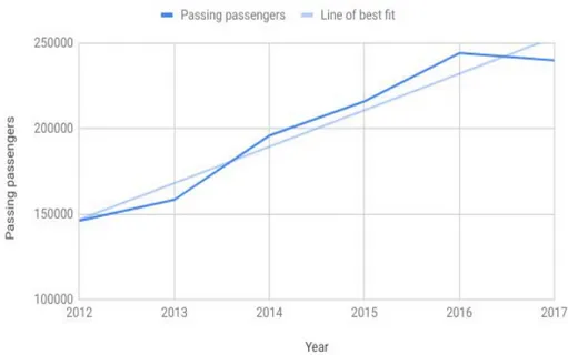
passed by that day and the results from the five others can be seen on the municipality home webpage (Infracontrol, 2018). The first measuring point was placed at “högskolan” [university] in 2005, and it was not until 2011 that four more measuring points were added, then one additional one in 2012, two in 2013 and lastly one in 2016. Since research indicates that younger and well educated individuals bicycle to a larger extent, using data between 2005 and 2011 when the observations where only from the local university measuring point might lead to overestimation (Xing et al, 2010; Caufield & Leahy, 2011; Rietveld & Daniel, 2004). To avoid this, assessments from 2012 and forward are displayed in the figure 6 (averages of each year), but it could be noted that during the time period 2005-2012, excluded for reasons mentioned above there was also a continuous increase in bicycles. What can be seen in the graph below is that there was a strong positive trend of bicycles passing the measuring points all the way up until 2016-2017, when there is a small decrease in bicycles. On average there was a 8% increase of passing bicycles/e-bikes every year.

Figure 6: The average amount of passing passengers in nine bicycle measuring points in Jönköping city during the time period 2012-2017 (Infracontrol, 2018)

Another piece of evidence comes from three surveys done by the municipality on the municipality employees which also indicate a positive cycling trend. In 2012 the percentage of employees cycling to work was 16% which increased to 17.5% in 2014 and then to 18% in 2016. The biggest increase was for e-bikes for which there was no question in 2012 but from 2014 to 2016 there was an increase of 165% (from 1.7% to 4.5%). It should be noted that the last survey was done in the end of 2016, therefore it also including some of the C2W- scheme participants which started in May of 2016. Lastly the municipality did their own evaluation of the C2W scheme in January 2017, (meaning that it included two opportunities of bicycle/e-bike leasing from 2016) in which a question whether individuals were planning to purchase a bicycle independently of the C2W scheme was included. The answers indicate that 19% of all

18

participants were planning on buying a bicycle/e-bikes the same year, and another 27% within a couple of years. These results could to some degree also be subject to social desirability bias, since cycling is something most often viewed as a positive (for the individual but also for the environment which is a common resource) especially in comparison with an automobile. This will not be addressed further in this thesis since the effect is most likely not large enough to skew the results but is worth mentioning. Almost all data on the trend of cycling in Jönköping point in the same direction; even without the C2W scheme there would probably have been an increase in bicycle/e-bike activity. The only exception to this is the data presented in figure 3, which indicates a 1% decrease in cycling on weekdays between 2009 and 2014. To what extent the increase is from individuals using their vehicles more often or from individuals buying a new vehicle and using it is impossible to say exactly. As a result of the increasing cycling trend, 20% of the effects calculated in section 7 will be removed from the final outcome.

Figure 7: Answers to the question “were you planning on purchasing a bicycle/e-bike independently of the C2W scheme?” asked to the municipality employees.

5.4 Data collection

Apart from literature and contact with the individuals who initiated the scheme at the municipality the main source of data was the participants in the scheme. In the fall of 2017, on two occasions (one week in between) an online-survey was sent out to the work email of all 2012 employees at the municipality who participated in the scheme. The survey consisted of 11 open-end-questions (seen in appendix E). There was a response rate of 21.3% (430/2012), even though some choose not to respond to all questions. The initial questions regarding the age and sex of the participants had similar results as the survey conducted by the municipality itself. The gender dispersion in this survey was 24% male, 74% female and 1% other and the age dispersion can be seen in figure 8 below.

19

Figure 8: The age dispersion of the participants in the C2W scheme.

5.4.1 Survey mode

Questions Average answer

How many months out of a year do you use your bicycle/e-bike: 31 weeks/year How many kilometres motoring (weekly) have you changed to cycling? 30.39 km/person

How many kilometres public transportation (weekly) have you changed to cycling? 10.5 km/person If you orders 2 bicycles and someone else except yourself is using one of they, please do

the same estimation as above for that person. How many kilometres motoring (weekly)

have he/she changed to cycling? 18.21 km/person

If you orders 2 bicycles and someone else except yourself is using one of they, please do the same estimation as above for that person. How many kilometres public transportation

(per week) do you estimate that he/she replaced with cycling? 31.82 km/person

How has you travel time changed weekly since you received your new bicycle/e-bike?

12 min 36 sec/person/week How has your amount of physical activity changed (daily) since you received your new

bicycle/e-bike?

14 min 30 sec person/day Table 1: Summary of the survey given to the participants in the C2W scheme, a full version of the survey can be seen in appendix D.

20

There were also questions regarding walking, but partly because the change in these transportation modes were small (from walking to bicycle/e-bike) and also that they have similar health/environmental effects they were not included in the thesis. The question regarding physical activity was included in an effort to address the possibility of substitution between transportation and other workout. One notable thing is that 24.8% reported no change in PA and many noted that they already had a bicycle since previously so a new vehicle did not change their PA level. The written elaborations do however indicate that there perhaps should have been a clearer distinction between cycling and other sorts of workout. It is unclear whether the respondents equivocated PA due to transportation to other kinds of workouts. Similar results as to change in PA were given for the change in travel time, where 24.6% reported that they had no change in travel time. Some participants noted that they had no change in either because they had a bicycle before the scheme and simply upgraded it. The participants who leased two vehicles were asked to estimate the effect for those who did not, these estimates are for obvious reasons more uncertain since they are second hand estimates. Despite this they were included since they are an effect of the scheme, and including them more likely creates a truer estimation of outcome then excluding them.

21

6. Costs and Benefits - Effects and Cost Calculations

This chapter overviews and explains the effects of the C2W scheme that are included in the CBA. The effects are divided into direct effects which affect the cyclist and indirect effects which affects society as whole (Krizek, 2007). Many times the effects overlap, meaning what is good for the individual is good for society as a whole and vice versa. The parameters excluded can be found in Appendix C.

CBA Parameter

Expected effect

on outcome Methodology to Quantify Effect Data Requirement Direct effects

Health

-Physical activity Positive

Change in vehicle km for all travel modes

Marginal cost estimates for health benefits and change in km travelled

-Noise pollution Positive

Change in vehicle km for all travel modes

Marginal cost estimates for noise pollution and

change in km travelled

-Local and Regional Air

Pollution Positive

Change in vehicle km for all travel modes

Marginal cost estimates for air pollution and change in km travelled

-Accidents Negative

Change in vehicle km for all travel modes

Marginal cost estimates for accidents and changes

in km travelled

Travel time Negative

Change in time spent travelling different modes

Marginal cost estimated for travel time and changes

in km travelled

Parking Positive Change in nr of parking occasions

Cost estimations for parking in Jönköping municipality and change

in nr of parkings

Vehicle purchase and

operation Positive

Change in vehicle km for all travel modes

Marginal cost estimates for Vehicle operation and change in km travelled for

each mode Indirect effects

Climate change Positive Change in vehicle kilometers

Marginal CO2 emission

cost and change in km travelled

Implementation costs Positive

Change in public spending by the municipality

Estimates in hours spend on campaign and average

hourly wage Absenteeism Positive

Change in absenteeism at

workplace Not empirically quantified

Infrastructure Positive

Change in vehicle km for all travel modes

Marginal cost estimates for infrastructural

deterioration Table 2: All parameters included in the CBA; the methodology to quantify them and what data was used.

22

6.1 Health

There are many ways in which AT can affect an individual’s health. There are firstly possible physical benefits such as decreases in cardiovascular disease, diabetes, cancer, obesity, musculoskeletal conditions, infectious and respiratory diseases. If an increase in AT also entails a decrease of motorised transportation there are other positive health effects such as less noise pollution and regional and local air pollution. However, increased AT also have negative effects such as increased risk of personal injuries due to accidents. Social cost connected to extended life expectancy is outside the scope of this thesis and therefore not included.

6.1.1 Physical activity

The benefits from increased physical activity are well documented within many fields of research. The definition of physical activity and what time interval to stay active (in order to see positive impact) is debated but the recommended amount for an average adult is 30 min of daily moderate physical activity (WHO, 2010). The benefits of this type of activity can be seen in a decrease several diseases: cancer, osteoporosis, coronary heart disease, diabetes as well as in prolonged life and a decrease in all-cause mortality (Warburton et al, 2006; Reiner et al, 2013;).

Most evidence indicate that AT does indeed have positive effects on health, but the robustness of the evidence varies and there is still uncertainty about the dose-response relationship (Saunders et al, 2013; Gordon, 2017; Goodman et al, 2014; Wanner et al, 2012; Kelly et al, 2014). The question is not so much whether AT has positive health outcomes but rather how much it actually contributes to the total activity. If the cyclists already take the health benefit into consideration when making their travel choice, meaning if the cyclist substitute their already existing exercise regime with their cycling to work the health benefit has already been internalized and no additional benefit would be made (Börjesson & Eliasson, 2012). There are indications that AT to some degree substitutes other PA and if so, the positive effects of AT could be overestimated. However, no studies focus exclusively on the substitution between AT and other PA, and the substitution degree remain uncertain as a result, most studies assume zero substitution (Mueller et al, 2015; Genter et al, 2008; Kahlmeier et al 2011, Brown et al, 2016)).

Nonetheless, one study indicating the magnitude of a possible incorrect assumption was produced by Börjesson and Eliasson (2012) in which they conclude from surveying cyclist in Stockholm, Sweden that the effect could be up to 60% less than expected. They found that 52% of cyclists stated that exercise was the most important reason to choose bicycle (61% for individuals over years). Björklund and Mortazavi (2013) built on and extended the study by Börjesson and Eliasson (2012) and found that individuals who said that they would exercise

23

more if they did not cycle less (interpreted to mean that they gain additional health benefits from cycling) valued their time slightly higher than those who said that they would not exercise more if they did not cycle (interpreted to mean that they did not get additional health benefits). Even though the difference were small, it could read in favor for some internalisation of health benefits. In one of the only three rapports that estimates a C2W scheme they also found that as much as 50% of the participants did not increase their PA due to the scheme and as much as 6% even decreased the PA because the exchanged walking for cycling which is faster (Clarke et al, 2014). To avoid overestimating possible health effects the assumption of zero substitution will not be made in full in this thesis. This is partly due to the ambiguity within the literature but also due to the results of the survey conducted among the municipality employees where almost 25% indicated no change in their activity levels (for the remaining 75% the average was a 14.5 min/daily increase). Due to lack of data the substitution degree will be somewhat arbitrary based on the indication in the survey and 25% of the effect for both bicycles and e-bikes will be assumed already internalised. Further internalisation will be considered in the sensitivity analysis.

Transportation mode Marginal cost/benefit from PA ($/km)

Bicycle 0.29

E-bike 0.29

Automobile -

Public transportation -

Table 3: Summary of marginal cost/benefit from increased PA for all transportation modes (HEAT, 2018).

Bicycle

There are many studies linking not only increased physical activity in general to health benefits but bicycling specifically. One study by Hu et al (2007) which included 48,000 participants found that “moderate or high levels of occupational or leisure-time physical activity among both men and women, and daily walking or cycling to and from work among women are associated with a reduced 10-year risk of coronary heart disease”. In addition, Cavill et al (2008), Andersen et al (2000), Mueller (2015) and other studies discussed in the literature review (see figure 4 and appendix A) all find positive health outcomes from increased bicycle usage.

To calculate the health benefits from increased AT the commonly used health economic assessment tool (HEAT) for cycling and walking will be used (HEAT, 2018). Because of the complexity in assessing health effects WHO developed HEAT as a tool which uses the latest published economic valuations of transport projects and epidemiologic literature (Kahlmeier et al 2011). HEAT only accounts for economic impact of mortality (using value of statistical life; VSL), since the literature is less conclusive about the economics of morbidity, they argue it would lead to greater uncertainty to include it. The authors acknowledge that this is likely to

24

produce conservative estimates since it does not account for disease related benefits (Kahlmeier et al, 2011). The relationship between cycling and mortality is assumed to be linear, despite some evidence that the relationship is not completely linear it was considered “adequate within

the foreseen range of activity for HEAT” (HEAT, 2018). The tool takes regional differences

into consideration, in this case using the Swedish VSL of $45,457,031 (£3,990,000). No distinction was made between the level of physical ability amongst the participants not between the ages. Age and physical ability have opposite effects on the health benefits, with age the benefit is increasing and with physical ability the benefit is decreasing (NVV, 2005; PWC; 2009; Department for transportation; 2010). The physical ability amongst the participants is unknown but the age is not, nonetheless both were excluded from the calculations in the hopes of the effects somewhat cancelling each other out. For specific inputs in the HEAT calculation see appendix D.

E-bike

There are less studies on the health benefits form e-bikes compared to ordinary bicycles and the demanded level of physical effort, for the same travel distance, is undoubtedly lower. However, given the rising popularity of e-bikes, more and more research which measure the physical effort and thereby determining their health impact is being produced. The measurement most commonly used to measure physical activity is the metabolic equivalent of task (MET), where 1,0 MET represent the metabolic rate associated with being at rest. Haskell et al (2007) suggest that to promote and maintain health the exercise intensity should be at least 3,0 MET. Several studies have indicated that the average MET while riding an e-bike is well above 3 and most likely somewhere between 5-7 (Gojanovic et al, 2011; De Geus et al, 2007; Simons et al, 2009). Since these studies indicate that health impact from an e-bike is sufficiently high to produce desired health effect, the health effect will be assumed identical for bicycles and e-bikes.

Automobile and public transportation

Since motorised transport does not entail any physical activity these will not be considered in the estimation. But it should be noted that in some studies public transportation is denoted as an active transportation mode since it entails more physical movement then automobiles. But in this thesis they are both treated as non-active and no estimate is included.

6.1.2 Noise pollution

Noise pollution (and to some extent vibration which will not be treated separately) is one of the most common pollutants in the western world and a large amount of it is roadway noise (WHO, 2011). How noise affects us is dependent on the noises character (the quality of the noise such as its volume and frequency), surrounding environment, possible vibrations and

25

time of day. The effects of noise pollution are increased risk of cardiovascular disease, sleep disturbance, annoyance, cognitive impairment, metabolic outcomes, hearing impairment, tinnitus and lower quality of life, mental health and well-being (WHO, 2018).

Transportation mode Marginal cost due to noise pollution ($/km)

Bicycle -

E-bike -

Automobile $0.021

Public transportation $0.105

Table 4: Summary of all marginal costs due to noise pollution (Trafikverket, 2018; Strömmer, 2003)

Bicycle and e-bikes

Bicycles and e-bikes do make some noise while being operated but since the decibel of the noise produced is not high enough to have an effect on human health the damage cost is negligible and not included in the estimation.

Automobile

Noise pollution is especially a problem in bigger cities but is also becoming a problem in smaller cities that have larger roads passing through (Trafikverket, 2016). The exposure to roadway noise is usually over longer periods at lower volumes so it is primarily those circumstances that are considered when constructing cost assessment. With continuous roadway noise pollution (with an average dB of 55) there is an increased risk of cardiovascular disease and myocardial infarction, increased stress levels, difficulty to perceive speech and concentrate as well as worsened sleep and rest quality (Ising & Kruppa, 2004).

The most common way to measure noise exposure is to determine either an equivalent value (an average over a longer time period) or a maximum-value when specific vehicles pass. Trafikverket perform, in accordance with the EU Directive 2002/49/EC, regular noise assessments as well as produce noise maps. They estimate that around 1.4 million individuals in Sweden are during day hours exposed to equivalent levels above 55 dB (Trafikverket, 2018). The effect of roadway noise can be at least partly combated by constructing noise protection, which would reduce the effects on human health but post a cost category on its own. These costs are not considered in the marginal price of noise pollution, instead the assessment has been done using 50/50 outdoor and indoor effects with several different pricing methods. For sleep disturbance and effects on stress, hedonic valuation methods in the form of WTP for reduced noise pollution in the form of property value have been used. These methods do come with a certain degree of uncertainty, for example the interference effects of noise pollution could not be included in the price differences in the housing market, if potential buyers are not

26

able to observe them. Estimates for heart disease come from WHO who have used VSL as a price indication and then the added costs of Swedish health aftercare for individuals suffering from heart disease (Trafikverket, 2016).

When the cost of increased dB levels is determined by the methods mentioned above the marginal cost estimation (for an average automobile in an urban area) is exemplified in the formulas below:

10*Log(1+ 0.5*1/(365*X)) = 0.00000397 dB (2) 0.00000397*Y = Total cost

Total cost/the total length of the road network = marginal cost

(X) = the average yearly traffic flow for 24 hours (between 1100-1800) (Y)= the marginal cost of damage for the increase of 1dB (Strömmer, 2003). Trafikverkets cost estimates of roadway noise have varied with time, the latest estimation will be used here. The marginal cost for urban environment is divided into three: $0.019/km in sparsely populated areas, $0.021/km in middle populated area and $0.023/km in densely populated areas (Trafikverket, 2018). Since there is variation in the population density in Jönköping, the average estimate of $0.021/km will be used (Trafikverket, 2018).

Public transportation

The marginal cost for buses in urban areas is $0.105/km/person, this damage cost was estimates in the same way as for automobiles, with the exception that the damage caused by heavy vehicles was assumed to be seven times higher than for a normal automobile (Strömmer, 2003).

6.1.3 Local and Regional Air Pollution

Local and regional air pollution differ in definition, included substances as well as method of estimation. Local effects of traffic are the direct effects of air pollution close to the source and include health effects due to emissions of NOx, SO2 and VOC as well as contamination from PMm (Trafikverket, 2018). Regional effects are both direct and indirect effects in a relatively large area around the source. The direct effects are the same as for the local pollution, while the indirect effects are effects that occur because the initially emitted substance react with some other chemical creating a new substance which in turn has damaging effects such as acidification or over-fertilization (a process known as “the cocktail effect”). The substances included in the regional estimates are NOx, SO2 and VOC for both health and environmental

effects.

The local and the regional effect are estimated differently. To calculate the cost of the local effects there are two steps, the first step is estimating the exposure according to the formula below to find the exposure unit per kilo of emission in which (Fv) = ventilation factor, (B) =

27

population amount, (0.029) = given parameter (Trafikverket, 2018).

Exposure unit per kilo of emissions = 0.029 * Fv * B0.5 (3)

Depending on the location of the area and its population density, areas are assigned “ventilation factors” which are indicated on the map (figure 6), Jönköping municipality is located in area ventilation zone 3, and is therefore assigned the ventilation factor 1,1.

Figure 9 : Map of Sweden with five ventilation zones, Jönköping is marked with a red circle. (Trafikverket, 2018)

Ventilation zone Ventilation factor, Fv

1-2 1

3 1.1

4 1.4

5 1.6