Uncertainty analysis of the Standardized Precipitation Index in the
presence of trend
Antonino Cancelliere
Department of Civil and Environmental Engineering, University of Catania, Catania (Italy) Brunella Bonaccorso
Department of Civil and Environmental Engineering, University of Catania, Catania (Italy)
Abstract. The Standardized Precipitation Index (SPI) is an index widely used for drought
monitoring purposes. Since its computation requires the preliminary fitting of a probability dis-tribution to monthly precipitation aggregated at different time scales, the SPI value for a given year and a given month will depend on the particular sample of observed precipitation adopted for its estimation and in particular on the sample size. Furthermore, the presence of trend in the underlying precipitation will affect adversely the estimation of parameters, and therefore the computation of SPI.
Objective of the present paper is to investigate the variability of the SPI with respect to the size of the sample used for estimating its parameters, either in the case of stationary or non station-ary precipitation series. In particular, sampling properties of SPI, such as bias and root mean squared error (RMSE), are analytically derived assuming the underlying precipitation series without trend and normally distributed. Results related to the normal case can find application also in the case of other distributions, namely when sample data can be transformed into normal values (i.e. lognormal or cube root normal distributed data).
Moreover, sampling properties when precipitation is affected by trend are investigated by means of Monte Carlo simulation. Results indicate that SPI values are significantly affected by the size of the sample adopted for its estimation. In particular, while for the case of underlying stationary series, RMSE tends asymptotically to zero as sample size increases as expected, in the presence of a linear trend a minimum RMSE value can be determined corresponding to a specific sample size. This suggests that an optimal sample size (in RMSE sense) can be deter-mined, when the underlying series is affected by trend.
1. Introduction
The Standardized Precipitation Index (McKee et al.,1993) is one of the most widely applied tool for drought monitoring (Edwards and McKee, 1997; Hayes et al. 1999; Lloyd-Hughes and Saunders, 2002; Bonaccorso et al., 2003; Sonmez et al., 2005; Vicente-Serrano, 2006; Wu et al., 2007) and, more recently, for drought forecasting as well (Bordi et al., 2005; Mishra and Desai, 2005; Moreira et al., 2006; Cancelliere et al., 2007). Its major strength stems from the possibility to compare drought events in re-gions and areas with different climates, taking into account the different time scales at which the components of the hydrological cycle are affected by precipitation deficits.
The index is based on an equiprobability transformation of precipitation values ag-gregated at k-months into standard normal values, with k generally fixed according to the purpose of the analysis. In practice, computation of the index requires i) fitting a probability distribution to aggregated monthly precipitation series (e.g. k= 3, 6, 12, 24,
36 months), ii) computing for each value the non-exceedance probability and iii) deter-mining the corresponding standard normal quantile, which is the SPI value.
McKee et al. (1993) assumed aggregated precipitation gamma distributed and esti-mated parameters using maximum likelihood. Guttman (1998) discussed this assumption by analysing precipitation data from 1035 stations in the U.S. and concluded that, at least for the U.S. it would be preferable to use the Pearson type III distribution. Also, Lana et al. (2001) found that the Poisson-gamma distribution is suitable for modelling precipita-tion in Catalonia (Spain).
Regardless of the parametric distribution adopted, as a consequence of the procedure of parameter estimation, the SPI values will exhibit sampling variability, namely, the SPI for a given year and a given month will depend on the sample size of the observed series of precipitation. This implies a potential limitation when comparing index values based on sample series of different length.
Wu et al. (2005) investigated the effect of the length of precipitation record on SPI calculation by examining the correlation coefficients, the index of agreement and the consistency of dry/wet event categories between SPI values derived from different re-cord lengths of observed precipitation. Changes of the shape and scale parameters of the gamma distribution corresponding to different lengths of record were also investigated. They concluded that the longer length of record used in SPI calculation, the more reli-able the SPI values will be.
In the present paper the effect of the length of precipitation record on SPI calcula-tion is investigated by analyzing the influence of the sample size on the sampling prop-erties of the index, either in the case of stationary or non stationary precipitation series. In particular, explicit expressions of Bias and Root Mean Squared Error of SPI are de-rived under the assumption of aggregated precipitation normally distributed. It is also shown that such derived expressions hold true, when precipitation can be assumed nor-mally distributed after a monotonic transformation is applied (e.g. Box and Cox, 1964), as is the case for instance of lognormal distributed data.
Then, sampling properties of SPI are investigated by means of Monte Carlo simula-tion in the case when precipitasimula-tion is affected by trend.
Results indicate that SPI values are significantly affected by the size of the sample adopted for its estimation, both in the case of stationary and non stationary series. In particular, for the case of underlying stationary series, while the bias is close to zero re-gardless of the sample size, RMSE tends asymptotically to zero as sample size in-creases, as expected. On the other hand, in the presence of a linear trend, bias values di-verge from zero as both sample size and trend slope increase, while RMSE first de-creases until a minimum value is reached corresponding to a specific sample size and then increases again. This suggests that an optimal sample size (in RMSE sense) can be determined, when the underlying series is affected by trend.
2. The Standardized Precipitation Index
In order to derive the sampling properties of the SPI, it is worth recalling its formal definition. With reference to a periodic monthly precipitation series , where ν=1,...n is the year and τ=1,...,12 is the month, let’s define the backward aggregated se-ries of order k as:
(1)
Assume , for fixed τ identically distributed according to some cumulative den-sity function (cdf) . Then, the SPI value corresponding to a given value of
is defined as:
(2)
where is the inverse of a standard normal cdf with zero mean and unit variance. From such definition it follows that the SPI index is normally distributed with zero mean and unit variance. Practical computation of the SPI requires fitting a distribu-tion to an observed sample for fixed τ.
From a theoretical standpoint, the distribution of aggregated precipitation fol-lows directly from the distribution of monthly precipitation . For example, if is normally distributed, then will be also normally distributed. However such an analytical derivation may not be straightforward in other cases. Despite the theoretical possibility to derive analytically the distribution of from that of , in practice it is preferable (and easier) to choose a distribution for from a parametric family and estimate parameters directly from a sample of aggregated values. Following McKee et al. (1993), usually the gamma distribution is employed for such a task, although in prin-ciple, this may not apply to all cases.
The main sources of uncertainty in the computation of SPI index stems from the choice of the parametric probability distribution to fit aggregated monthly precipitation series, as well as from the estimation of the unknown parameters. In turn, the latter is influenced by the length of the sample adopted for estimating the parameters. The as-sessment of the relationship between precipitation sample length and corresponding es-timation error for SPI is the subject of the next paragraphs.
3. Sampling properties of SPI: normal distribution, no-trend case
For the sake of simplicity, the series will be hereafter denoted by , since we are interested in analysing the sampling properties of the SPI for fixed τ and k.Let aggregated precipitation , with ν=1, 2,..., n, be an independent and identically normally distributed process with mean µ and variance σ2, i.e.:
Y1, Y2,…,Yn N(µ,σ2) (3)
Let’s assume the mean µ and the variance σ2 are estimated by the Maximum
Like-lihood Estimation method (MLE), namely:
(5) where y1, y2,…,yn is a sample from (3). With reference to a generic observation Y, not
included in the estimation sample, the corresponding estimated SPI is given by the simple equation:
(6)
as descends directly from Eq. (2) when is normally distributed. The true SPI value Z, based on the population mean and standard deviation of the underlying series is:
(7)
Therefore, the sampling variability of the SPI can be characterized by investigating the distribution of the following random variable as a function of the estimation sample size n:
(8) The random variable D is the difference of two random variables: the first is obvi-ously normally distributed with zero mean and unit variance. To derive the distribution of the second r.v. , it has to be observed that for the normal distributed variables, the sample mean and the sample variance S2 are independent (see for example Mood et al., 1974), and, in our case Y is independent of both, since it is not included in the esti-mation sample. Furthermore, for i.i.d. normal distributed random variables the follow-ing well known results hold (Mood et al., 1974):
(9) and
(10)
The r.v. is therefore the ratio of a normal r.v. to the squared root of a χ2 r.v. and thus, after an appropriate rescaling, it is distributed as a Student’s t (Mood et al., 1974). Indeed, it can be shown that:
(11)
From Eq. (11), it follows that and .
Analytical derivation of the distribution of D is not an easy task, since D is the dif-ference of two dependent r.v., with a standard normal and a Student’s t as marginal dis-tributions, respectively. Nonetheless, the first two moments of D can provide enough in-formation to characterize the sampling variability of the SPI, since they allow to com-pute the bias and the Mean Squared Error (MSE) of estimation, as:
(12) and
(13) In practice it is preferable to use the Root Mean Squared Error (RMSE) of estima-tion which can be computed by taking the square root of the MSE:
(14) The bias term can be computed as:
(15) since both expectations are zero. Thus, in the normal case, the SPI estimator given by Eq. (6) is unbiased. As a direct consequence, the MSE of estimation coincides with
.
On the basis of Eq. (13), the MSE can be rewritten as:
(16) The first term in the above equation is obviously 1. The second term, as it has been
shown previously, is equal to .
The covariance term in Eq. (16) can be rewritten as:
(17)
The second term is obviously zero, since the observation Y is not included in the es-timation sample, and therefore it is uncorrelated with the sample mean or the sample standard deviation S.
By means of conditional expectation concepts, the first covariance term in Eq. (17) can be rewritten as:
(18)
The latter expectation can be computed by reminding that S2 is distributed according to
a rescaled χ2 distribution (Eq. (10)) and therefore it follows:
(19) Finally, combining Eqs. (16), (18) and (19), it follows that:
(20) thus
(21)
It can be inferred from Eqs. (20) and (21) that, in the normal case, the MSE of esti-mation of SPI does not depend on the parameters µ and σ2 of the underlying variable,
but only on the sample size n.
Equations (15) and (21) have been verified by means of Monte Carlo simulation. In particular, for a fixed sample size n, 50000 series of length n have been generated out of a standard normal distribution and, each time, two values of SPI corresponding to a normal variable have been estimated: the first, using the mean and variance of the sam-ple, and the other assuming the population mean and variance, namely 0 and 1 respec-tively. Then, RMSE has been computed as the average squared difference between the two estimates. Note that the choice of the standard normal as parent distribution for the Monte Carlo simulation is not limiting since, as shown previously, Bias and RMSE do not depend on the mean and standard deviation of the distribution. Thus, using a non-standard normal distribution would lead to the same results.
In Figure 1, RMSE given by Eq. (21) and observed RMSE, computed by simulation, are plotted versus the sample size n.
Figure 1. Theoretical (Eq. 21) and estimated (from simulation) RMSE of SPI for the normal distribution case
The plot indicates very good agreement between RMSE computed by Eq. (21) and those computed by simulation, thus confirming the validity of the derived analytical ex-pressions.
From the plot it can be inferred that the RMSE decreases with the sample size. In particular, the RMSE is about 0.24 for sample size 30, while it is 0.15 for sample size 70.
4. Sampling properties of SPI: other distributions, no-trend cases
If Yν is not normally distributed, the SPI must be computed according to Eq. (2), which can be rewritten by explicitly taking into account the parameters of the distribu-tion, here indicated generically by a parameter vector Θ :(22)
In practice, the parameters Θ of the underlying distribution are unknown and there-fore they will be estimated as . As a consequence, the estimated SPI will take the form:
(23)
Although in principle, the sampling variability of the SPI can again be characterized by the deviation between the true SPI and the estimated one (see Eq. (8)), in practice derivation of the distribution of is generally rather cumbersome, which hinders the possibility of an exact analytical approach.
Nonetheless, it can be shown that Eq. (15) and Eqs. (20)-(21) are valid also for a large class of non-normal distributions, namely when data can be normalized by means of a monotonic transformation, e.g. Box-Cox (Box and Cox, 1964) among others.
More specifically, let’s assume that there exist a monotonic function g(⋅) such that the transformed precipitation is normally distributed with mean and standard deviation . It follows:
(24) and Eq. (22) yields for the true SPI:
(25)
Estimation of the parameters ( , ) can be carried out by means of MLE, namely by computing the sample moments in the transformed domain, leading to:
(26) (27) and the error of estimation of the SPI is:
(28)
Note how the previous equation resembles Eq. (8) since Y* is normally distributed by definition and and are again sample mean and sample standard deviation of normal variables. Thus, the statistical properties of D are the same as in the previous case, and in particular Eqs.(15), (20) and (21) are still valid. It may be worthwhile to note that the same equations can still be considered valid, with good approximation, also in the case of gamma distributed precipitation, since it is well known that the gamma distribution is well approximated by the normal cube root distribution (Wilson and Hilferty, 1934), i.e. when Y*=Y1/3.
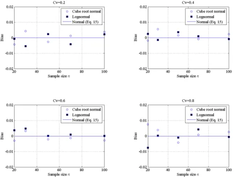
In order to verify the previous findings, two sets of numerical experiments have been carried out by generating aggregated precipitation using the log normal and normal cube root distributions respectively. Then, for each distribution, after computation of corresponding SPI values, the bias and RMSE of the resulting SPI have been estimated numerically, following a similar procedure already outlined for the normal case, consid-ering different sample sizes n and parameters Θ. In particular, different parameter sets have been considered by fixing several coefficients of variation of the distribution, and deriving the corresponding parameters.
In Figure 2 the bias computed by simulation for the two distributions are plotted versus the sample size for different . It can be inferred that, for practical purposes, they are negligible and therefore the estimation can be assumed unbiased. Furthermore, the spread of the bias around the zero value do not seem to depend on the different
.
Figure 2. Bias of estimation of SPI for the gamma distribution case (circles) and the lognormal distribu-tion case (dots)
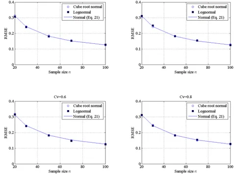
In Figure 3 the RMSE’s of estimation obtained by simulation are plotted versus the sample size for different . For the sake of comparison, the RMSE’s computed by means of Eq. (21) for the normal case are also plotted by continuous line. As expected, a comparison between the RMSE’s derived for the normal case and the numerical val-ues obtained for the other two distributions reveals a very good fitting of the theoretical line to the numerical RMSE, which confirms the possibility to apply Eq. (21) also to non normal data which can be transformed into normal values. Also, RMSE computed from generated values do not depend on the coefficient of variation Cv, as was expected
since Eq. (21) does not depend on the parameters of the underlying distribution.
Figure 3. RMSE’s of estimation of SPI for the gamma distribution case (circles) and the lognormal dis-tribution (dots)
5. Sampling properties of SPI in the presence of trend
The analytical expressions of Bias and RMSE of SPI previously derived can be ap-plied to stationary normal precipitation series (section 3), as well as to stationary non normal series for which a normalizing transformation is feasible (section 4).
Nonetheless, the question arises regarding how the sampling properties of SPI vary when a non stationary series of precipitation is adopted for its computation, for instance when precipitation is affected by trend.
Although in principle, analytical expressions of the sampling properties can be de-rived also in the case of a trend component in the underlying series, in the present paper only the preliminary results related to Monte Carlo experiments are reported.
In particular, as done previously, numerical simulations have been carried out to compute the bias and RMSE of the SPI, by generating this time precipitation series of different sample sizes n normal distributed and affected by a linear trend,.
• first, a series of n+1 values are sampled by generation from a normal distribution with mean zero and variance s2;
• then, a linear trend is added to the sample series by considering different slopes b; • the “true” SPI corresponding to the value yn+1 in the sample is computed as:
since the term b⋅(n+1) is the true mean, having assumed an arbitrary mean equal to zero at time t=0;
• the estimated SPI corresponding to the value yn+1 is computed by using the sample
mean and sample standard deviation based on the previous n values, that is:
• the procedure is repeated by generating 5000 series;
• the mean of the difference and of the squared difference between the estimated and the “true” SPI values are computed, yielding an estimate of the bias and MSE; • the whole procedure is then repeated for different n.
In Figure 4 and Figure 5, the values of bias and RMSE obtained by simulation are plotted versus the sample size for different slopes. For the sake of generality, the slope values are expressed as ratio to the standard deviation s, namely b*=b/s.
As it can be observed from Figure 4, the larger the sample size n, the more bias val-ues diverge from zero, with positive bias for b*<0 and negative otherwise. Furthermore, for a fixed sample size, the difference from zero enlarges as the absolute value of b* in-creases. This is expected due to the fact that as more past values are included in the es-timation sample, the estimate of the mean and standard deviation will be affected by in-creasing error due to the trend.
However, as shown in Figure 5, the RMSE exhibit a rather different behaviour than bias, since, as sample size n increases the RMSE’s first decreases and then increases again. Therefore, a minimum value of RMSE can be determined for each considered slope b*≠0 corresponding to a given sample size. In particular, the latter reduces as the absolute values of b* increases, e.g. ranging from n=55 for b*=±0.5% to n=15 for b*=±4 %.
6. Conclusions
In the present paper the sampling variability of the SPI with respect to the size of the sample used for estimating the parameters of the probability distribution of aggregated precipitation has been investigated both in the case of stationary or non-stationary (e.g. affected by linear trend) series. In particular, sampling properties of the index, such as bias and RMSE, have been derived analytically for the case of stationary normally dis-tributed precipitation.
Figure 4. Bias of estimation of SPI in the case of normal distributed precipitation series affected by a lin-ear trend with different slope parameter b*
Figure 5. RMSE’s of estimation of SPI in the case of normal distributed precipitation series affected by a linear trend with different slope parameter b*
Moreover, it has been shown that the same expressions are applicable also for the case of a broad class of distributions, namely when data can be normalized by means of a monotonic transformation. The derived expressions reveal that SPI is unbiased, while, as expected, the RMSE tends asymptotically to zero as sample size increases. In this
case, it can be concluded that RMSE cannot be considered negligible for sample sizes in the order of 20-30 data.
On the other hand, simulation experiments have revealed that when the estimation sample is affected by a linear trend, bias values diverge from zero as both sample size and trend slope increase, while RMSE first decreases until a minimum value is reached corresponding to a specific sample size and then increases again. Therefore, it appears that an optimal sample size (in RMSE sense) can be determined, when the underlying series is affected by trend.
Further researches are ongoing in order to derive analytical expressions of the sam-pling properties of the SPI for non stationary series.
Acknowledgements. The financial support of the national project MIUR-PRIN 2007,
“Drought indicators and models for the definition of triggering levels for measures to prevent water emergencies in water supply systems” is gratefully acknowledged.
References
Bonaccorso, B., Bordi, I., Cancelliere, A., Rossi, G., Sutera, A. (2003). Spatial Variability of Drought: An Analysis of the SPI in Sicily. Water Resources Management, 17 (4): 273-296. Bordi, I., Fraedrich, K., Petitta, M., Sutera, A. (2005). Methods for predicting drought
occur-rences, in Proceedings of the 6th International Conference of the European Water Re-sources Association, Menton, France, 7-10 September 2005.
Box, G.E.P., Cox, D.R. (1964). An analysis of transformations. Journal of the Royal Statistical
Society, Series B 26 (2): 211–252.
Cancelliere, A., Di Mauro, G., Bonaccorso, B., Rossi, G. (2007). Drought forecasting using the Standardized Precipitation Index. Water Resources Management, 21(5): 801-819.
Edwards, D.C., McKee, T. (1997). Characteristics of 20th century drought in the United States at multiple scales. Atmospheric Science Paper No. 634, May; 1–30.
Guttman, N.B. (1998). Comparing the Palmer Drought Index and the Standardized Precipitation Index. Journal of the American Water Resources Association, 34(1): 113-121.
Hayes M, Wilhite D, Svoboda M, Vanyarkho O. (1999). Monitoring the 1996 drought using the standardized precipitation index. Bulletin of the American Meteorological Society, 80(3): 429–438.
Lana, X., Serra, C., Burgueno, A. (2001). Patterns of monthly rainfall shortage and excess in terms of the standardized precipitation index for Catalonia (NE Spain). International
Jour-nal of Climatology 21(13): 1669–1691.
Lloyd-Hughes, B., Saunders, M.A. (2002). A drought climatology for Europe. International
Journal of Climatology, 22: 1571–1592.
Mishra, A.K., Desai, V.R. (2005). Drought forecasting using stochastic models. Stochastic
En-vironmental Research and Risk Assessment, 19: 326–339.
Mood, A.M., Graybill, F.A., Boes D.C. (1974). Introduction to the theory of statistics. McGraw-Hill Series in Probability and Statistics.
Moreira, E.E., Paulo, A.A., Pereira, L.S., Mexia, J.T. (2006). Analysis of SPI drought class transitions using loglinear models. Journal of Hydrology, 331(1-2): 349-359.
McKee T., Doeskin N., Kleist, J. (1993). The relationship of drought frequency and duration to time scales. Proceedings of the 8th Conference on Applied Climatology; January 17-22.
Sonmez, F.K., Komuscu, A.U., Erkan, A., Turgu, E. (2005). An analysis of spatial and temporal dimension of drought vulnerability in Turkey using the standardized precipitation index.
Natural Hazards, 35: 243–264.
Vicente-Serrano, S. M. (2006). Spatial and temporal analysis of droughts in the Iberian Penin-sula (1910-2000). Hydrological Sciences Journal, 51(1), 83–91.
Wilson, E.B., Hilferty, M.M. (1931). The Distribution of Chi-Squares, Proceedings of the
Na-tional Academy of Sciences, 17: 684–688.
Wu, H., Hayes, M.J., Wilhite, D., Svoboda, M.D. (2005). The effect of the length of record on the Standardized Precipitation Index calculation. International Journal of Climatology, 25: 505-520.
Wu, H., Svoboda, M., Hayes, M., Wilhite, D., Wen, F. (2007). Appropriate application of the Standardized Precipitation Index in arid locations and dry seasons. International Journal of