Distribution of velocities in a cross section using the logD method:
Application to a cross section of the Wainiha River
Robert T Milhous
Hydrologist, Fort Collins, Colorado 80526
Abstract. The logD method distributes velocities across a transect (cross section) uses the equation . In the equation d is the depth at a location in the cross section, S is the slope, α is an empirical parameter, k is the absolute roughness height and C is a constant (32.61 for traditional English, and 18.00 for metric units). Typical value of α is 10.96 (based on theoretical considerations), and 4.70 (based on empirical measurements). The distribution of velocities in a cross section is used in the Physical Habitat Simulation System (PHABSIM) to calculate physical habitat for aquatic animals. The logD method is an effective method for
calculation of the velocity distribution and helps reduce problems associated with the simulation of velocities at the edges of a channel. The method requires a consistence approach to the selection of the roughness heights. Roughness heights determined from measured velocities may not have a physical meaning but if roughness heights based on measured heights are used they must be used through out the cross section and not mixed with roughness heights determined from measured velocities.
1. Introduction
The Physical Habitat Simulation System (PHABSIM) developed for use in instream flow studies uses the equation:
to calculate physical habitat where HA(j) is the physical habitat area for a specific life stage of a species of aquatic animal at discharge Q(j). The summation is over m cross sections in a study reach and p(i) cells in cross section i. The other terms are: A(h,i,j) is the channel area associated with location h of cross section i at discharge j, v(h,i,j) is the velocity at location h of cross section i at discharge j, d(h,i,j) is the depth at location h of cross section i at discharge j, and CI(h,i) is an index of a channel characteristic at location h of cross section i. The channel index does not vary with discharge. The function f[ ] weights the channel area for the value of the channel area for the aquatic animal and is specific to a species and life stage. For details about PHABSIM and the habitat area equation see Milhous, Updike, and Schneider (1989). Sometimes the channel area is a pseudo-area based on a system of cross section weights and sometimes an area based on the distances between cross sections (see Milhous et al, 1989).
The Manning’s equation for the velocity in a cross section is:
(
( / ))
log d k Sd C v= a[
]
å
å
= ==
m i i p hi
h
CI
j
i
h
d
j
i
h
v
f
j
i
h
A
j
HA
, 1 ) ( , 1}
)
,
(
),
,
,
(
),
,
,
(
)
,
,
(
{
)
(
RS R n C V u úû ù êë é = 1/6where V is the cross-sectional velocity, R the hydraulic radius, S the energy slope, n the Manning’s roughness of the cross section, and Cu is a constant depending on the units (1.0
for metric units and 1.49 for traditional English units).
The equation used to calculate the velocity distribution in a cross section uses the Manning’s equation at each location in a cross section where velocities are needed for habitat simulation. The analysis replaces the cross-sectional hydraulic radius with the depth at the location and the overall Manning’s roughness with a roughness for the location. The equation is:
The velocity, v’(h,i,j) is an initial estimate of the velocity at location h in cross section i that must be adjusted to make the discharge calculated using the calculated velocities to be the same as the known discharge Q(j). All the velocities in a cross section must be
adjusted to give the discharge Q(j). Therefore, the velocities are adjusted by a velocity adjustment factor. The equation for the velocity adjustment factor is:
where VAF(i,j) is the velocity adjustment factor for the velocities in cross section i at the discharge j, a(h,i,j) is the cross-sectional area of cell h of cross section i at discharge j, and initial calculation of the velocity in the cell is v’(h,i,j). (The area is defined by the
distances between measurement points) The final calculation of the velocities uses the velocity adjustment factor to adjust the individual cell velocities using the equation:
The velocity, v(h,i,j) is used in the calculation of the habitat area. For details on the calculation process using velocity adjustment factors, see Milhous, Updike, and Schneider (1989).
This paper presents an approach to the calculation of velocities in cross sections using the logD method proposed by Diez-Hernández (2004). The logD method, in effect, makes the Manning’s roughness a function of discharge.
2. The LogD Method for Distributing Velocities in a Cross Section
A method for the distribution of velocities has been proposed by Diez-Hernández (2004) based on the Prandt-von Karman velocity distribution law. The form of the equation present by Diez-Hernández is:)
(
)
,
,
(
)
,
,
(
)
,
(
)
,
,
(
1/6 'd
h
i
j
d
h
i
j
S
i
i
h
n
C
j
i
h
v
uú
û
ù
ê
ë
é
=
å
==
) ( , 1 '(
,
,
)
*
)
,
,
(
)
(
)
,
(
i p ka
h
i
j
v
h
i
j
j
Q
j
i
VAF
)
,
,
(
*
)
,
(
)
,
,
(
h
i
j
VAF
i
j
v
'h
i
j
v
=
where, Ui is the average velocity, hi is the depth, g is gravitation acceleration, So is the
energy slope, and ki is absolute roughness in the same units as the other terms in the
equation. Ui, hi, and ki are all at location i in a cross section. Rearranging the equation to
give the equation used to calculate the velocity at each location where velocities are needed in a reach gives the equation:
where k(h,i) is an element of the array of absolute roughness for the reach and the other terms are as defined above.
In physical habitat simulation the velocities are used in the same way as described in the introduction. The absolute roughness array is determined in the model calibration process.
The use of the logD method to calculate the velocities in a single cross section of the Wainiha River on the island of Kauai, Hawaii, is the topic of the following sections of this paper.
3. The Wainiha River Cross Section
In this section data for one cross section of a river is used to investigate the
characteristics of the logD method of distributing velocities in a cross section. The cross section is the first cross section in a data set for the Wainiha River on the island of Kauai in Hawaii. The data was collected from 29 June – 1 July 1984 by Ken Bovee and a crew from the U.S. Fish and Wildlife Service (Ford, Chow, Yuen and Kinzie). The reach measured is just upstream from the Wainiha estuary. The cross section measurements and measured velocities at a discharge of 103 cfs are presented in Figure 1.
For the cross section shown in Figure 1 the cross-sectional Manning’s roughness was calculated to be 0.056 based on a hydraulic radius calculated as the cross-sectional area divided by the wetted perimeter and 0.060 using an area weighted hydraulic radius. The measured discharge is 103 cfs and water surface elevation is 92.50 feet. The absolute roughness calculated for the cross section is 2.024 feet (0.617 meters) based on the usual hydraulic radius and 2.436 feet (0.742 meters) based on an area weighted hydraulic radius.
The velocity equation used in the simulation of the velocity distribution can be
rearranged to give an equation for the Manning’s roughness associated with each vertical. The equation is:
ú
û
ù
ê
ë
é
÷÷
ø
ö
çç
è
æ
=
)
,
(
)
,
,
(
96
.
10
log
)
,
,
(
)
(
75
.
5
)
,
,
(
'
i
h
k
j
i
h
d
j
i
h
d
i
gS
j
i
h
v
)
(
)
,
(
)
,
(
)
,
(
)
,
(
d
h
i
1/6d
h
i
S
i
i
h
v
C
i
h
n
c c c uú
û
ù
ê
ë
é
=
where dc(h,i) is the depth at location i at the calibration discharge, and vc(h,i) is the
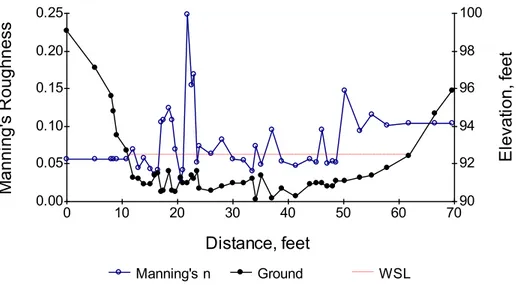
measured velocity at location i at the calibration discharge. The slope, S(i), is assumed to be constant across the cross section. The Manning’s roughness, n, calculated from the velocity data shown on Figure 1 is presented in Figure 2. The Manning’s n for dry cells was estimated as the average of the three wet cells nearest to the dry cell.
The Manning’s roughness has been called a distribution factor because the calculated values based on a set of velocities measured at a cross section are used to distribute the velocities across a section at unmeasured discharges. Best practice is to determine the water surface elevations as a separate activity from distributing velocities across the cross section.
Figure 1. Cross section 0.0 of an IFG4 data set for the Wainiha River on the island of Kauai. The velocities are for a discharge of 103 cfs and water surface elevation of 92.50 feet.
Figure 2. Calculated Manning’s roughness at cross section 0.0 of a data set for the Wainiha River on the island of Kauai. The roughness was calculated using velocities measured at a discharge if 103 cfs and water surface elevation of 92.50 feet.
0.0 0.5 1.0 1.5 2.0 2.5 3.0 90 92 94 96 98 100 0 10 20 30 40 50 60 70 V e lo ci ty, fp s E le va tio n , f e e t Distance, feet Velocity Ground WSL 0.00 0.05 0.10 0.15 0.20 0.25 90 92 94 96 98 100 0 10 20 30 40 50 60 70 M a n n in g 's R o u g h n e ss E le va tio n , f e e t Distance, feet Manning's n Ground WSL
4. Application of the logD method to the Wainiha River cross section
An application of the logD method to the Wainiha River cross section is presented in this section. The first task is the calibration of the logD equation to the Wainiha River cross section.4.1. Calibration
The equation used to calculate the absolute roughness for each measurement location (vertical) is obtained by rearranging the logD velocity equation. This equation is:
where dc(h,i) is the depth at the vertical for the calibration discharge, vc(h,i) is the
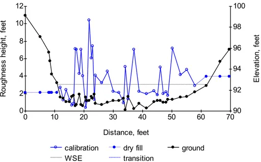
measured velocity at the vertical, g is the gravitational acceleration, and S(i) is the energy slope for the cross section. A velocity model for simulation of velocities over a range of discharges based on the logD equation is calibrated by determining the absolute roughness for each vertical based on an array of measured velocities. The results for the Wainiha River cross section are presented in Figure 3.
The measured velocities are not available for all points in the cross section. Simulation of velocities at discharge larger than the calibration discharge requires estimation of the roughness height at points above the water surface elevation at the calibration discharge. For the velocity model of the Wainiha cross section the roughness height used for points above the calibration water surface elevation was the average of the nearest three
calibration roughness heights; this was 3.94 feet for the three verticals on the right and 2.12 feet for the six verticals on the left. These are labeled ‘dry fill’ in the figure. Other values could be selected in the selected. There is a discussion about the selection Manning’s roughness values for dry locations in Milhous, Updike, and Schneider (1989) that applies also to the selection of absolute roughness values.
4.2. Simulation
The water surface elevation at a discharge of 500 cfs was determined to be 95.37 feet in previous analysis. When using the Physical Habitat Simulation System the calculation of the velocity distribution in cross sections follows the simulation of water surface elevation. The calibration roughness heights and the roughness heights estimated for the dry verticals were used to determine the velocities at the 500 cfs discharge. The results are in Figure 4.
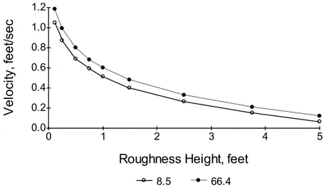
The selection of a roughness height is most important on the edges were the cells are dry at the calibration discharge. Figure 5 shows how the simulated velocities vary with the assumption of roughness heights for the dry cells. The roughness heights selected for the
}]
)
(
)
,
(
75
.
5
/{
)
,
(
[
10
)
,
(
96
.
10
)
,
(
i
S
i
h
gd
i
h
v
c
c ci
h
d
i
h
k
=
dry cells in the calculations leading to Figure 5 was the same for all dry cells compared to 2.12 feet on the left and 3.94 feet on the right estimated from the nearest three wet cells.
Figure 3. Roughness heights calculated for a cross section of the Wainiha River just upstream of its Estuary on Kauai. The calibration discharge was 103 cfs at a water surface elevation of 92.5 feet. The ‘dry fill’ locations are verticals above the water at the calibration discharge. (1 foot = 0.3048 meters)
Figure 4. Calculated velocities at a discharge of 500 cfs for a cross section of the Wainiha River just upstream of its Estuary on Kauai. The locations where the roughness heights were estimated from the nearest three wet cells are labeled ‘dry fill’.
0 2 4 6 8 10 12 90 92 94 96 98 100 0 10 20 30 40 50 60 70 Ro ug hn es s he ig ht , fe et El ev at io n, f ee t Distance, feet
calibration dry fill ground
WSE transition 0.0 0.5 1.0 1.5 2.0 2.5 3.0 3.5 4.0 90 92 94 96 98 100 0 10 20 30 40 50 60 70 V e lo ci ty, fe e t/se c E le va tio n , f e e t Distance, feet
calibrated dry fill transition
Figure 5. Velocity calculated for the two edge cells at a discharge of 500 cfs in the Wainiha River cross section as related to the assumption of the roughness heights for the dry cells at the calibration discharge of 103 cfs. The left cell is at 8.5 feet and the right at 66.4 feet. The velocity distribution for a discharge less than the calibration discharge is presented in Figure 6. The velocity can be negative for very shallow depths when the roughness height is larger than the 10.96 times the depth. There are at least three possible ways of dealing with these situations. These are:
1) for set the velocity to zero (0.0)
2) for calculate the velocity using the equation:
simplified the equation is:
3) also for use the equation:
The last equation was determined by placing a limit on the Manning’s roughness and using this to replace the depth. The third equation was used to calculate the velocities in Figure 6. 0.0 0.2 0.4 0.6 0.8 1.0 1.2 0 1 2 3 4 5 V e lo ci ty, fe e t/se c
Roughness Height, feet
8.5 66.4 96 . 10 / ) ,. ( ) , , (h i j k h i d £
(
1.1* ( , )/10.96)
) , , (k i j k k i d £ ) ) , ( 96 . 10 ) , ( 96 . 10 * 1 . 1 log( ) ( ) , , ( 75 . 5 ) , , ( i h k i h k i S j i h gd j i h v = ) 1 . 1 log( ) ( ) , , ( 75 . 5 ) , , (hi j gd h i j S i v =(
1.1* ( , )/10.96)
) , , (p i j k p i d £(
( , , )/(1.1 ( , )))
log(1.1) ) ( ) , , ( 75 . 5 ) , , (p i j gd p i j S p d p i j k p i 16 v =Figure 6. Calculated velocities at a discharge of 30 cfs for a cross section of the Wainiha River just upstream of its Estuary on Kauai. The locations where the roughness heights are larger than 9.96 times the depth are marked as limited. (9.96 = 10.96/1.1 – see text.)
5. Calculation of Manning’s Roughness using the logD method.
The use of the logD method of velocity distribution in a cross section within the Physical Habitat Simulation System (PHABSIM) can be done effective by using the logD method to calculate the Manning’s roughness, n instead of the velocity directly.The Manning’s equation is equated to the logD equation and eliminated to give the equation:
this can be rearranged to give an equation for the Manning’s roughness calculated from the absolute roughness. The resulting equation is:
0.0 0.5 1.0 1.5 2.0 2.5 3.0 3.5 4.0 90 91 92 93 94 95 96 97 98 99 100 0 10 20 30 40 50 60 70 V e lo ci ty, fe e t/se c E le va tio n , f e e t Distance, feet calibrated ground WSE limited ) , , ( ) (i d h i j S
ú
û
ù
ê
ë
é
÷÷
ø
ö
çç
è
æ
=
)
,
(
)
,
,
(
96
.
10
log
75
.
5
)
,
,
(
)
,
(
6 / 1i
h
k
j
i
h
d
g
j
i
h
d
i
h
n
C
uú
û
ù
ê
ë
é
÷÷
ø
ö
çç
è
æ
=
)
,
(
)
,
,
(
96
.
10
log
75
.
5
)
,
,
(
)
,
(
6 / 1i
h
k
j
i
h
d
g
j
i
h
d
C
i
h
n
uthis equation gives a Manning roughness that varies with discharge as the depth changes. It is the above form of the logD method that is considered in this section.
The 10.96 in the velocity equation is empirical. Limerinos (1970) developed a bunch of equations for Manning’s roughness. One of these was used to determine the Manning’s roughness and is the following equation:
where R is the hydraulic radius in feet, and d84 is the size, in feet, of the substrate where
84% of the particles are smaller based on the intermediate diameter (the diameter from sieve analysis or the Wolman procedure using a gravelometer). The equation can be transformed to a form that can use both metric and traditional English units; the result is:
The Limerinos paper is not clear about the method used to determine the 5.67 (compared to 5.75 in the logD equation and 3.80 (compared to 10.96) in the equation above. If we replace the 3.80 with a variable, α, and replace 5.66 with 5.75 the equation for the Manning’s roughness is:
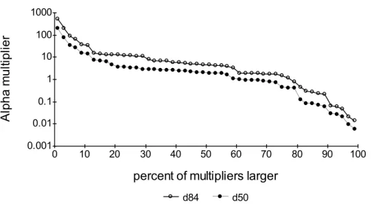
The α-term is called the alpha multiplier herein. Data in Limerinos was used to
calculate the value of the alpha multiplier. The range is 196 – 0.006 with a median of 4.70 (see Figure 7). Thirty eight percent of the values are between 10.96 and 1.85.
÷÷
ø
ö
çç
è
æ
+
=
84 6 / 1log
2
16
.
1
0926
.
0
d
R
R
n
ú
û
ù
ê
ë
é
÷÷
ø
ö
çç
è
æ
=
84 6 / 180
.
3
log
67
.
5
d
R
g
R
C
n
uú
û
ù
ê
ë
é
÷÷
ø
ö
çç
è
æ
=
84 6 / 1log
75
.
5
d
R
g
R
C
n
ua
Figure 7. Frequency of the alpha parameter as related to the percent larger for both the d84 and d50
sizes of the bed surface. The median value of alpha based on the d84 size is 4.70 and 1.94 based on
thed50 size.
Table 1. Variation of the roughness height for a cross section of the Wainiha River just upstream of its Estuary on Kauai as related to alternative assumptions of the alpha multiplier. The
roughness height was calculated from the area weighted hydraulic radius. (1 foot = 0.3048 meters)
Alpha multiplier roughness height, feet Ratio
10.96 2.434 4.503
4.70 1.044 4.502
3.80 0.844 4.502
1.85 0.411 4.501
Alternative values of the alpha parameter were used to calculate the associated roughness heights; these are presented in Table 1. The ratio in Table 1 is the alpha multiplier divided by the roughness height. The ratio is constant (with some round off difference) which means the vertical velocities will be the same no matter what value of the alpha parameter is used. There can be a difference if the value of the roughness height used in the dry cell is not consistent with the calibration roughness heights (i.e. use a d84
for the dry verticals when the calibration roughness heights are much larger as is probable for the Wainiha River cross section). In some situations the roughness heights are not from calibration to a set of velocities but selected by the analyst. The selection of the alpha multiplier will have an impact on the velocities simulated – especially on the edges (see Figure 8). 0.001 0.01 0.1 1 10 100 1000 0 10 20 30 40 50 60 70 80 90 100 Al p h a m u lti p lie r
percent of multipliers larger
Figure 8. Calculated velocities for a discharge of 500 cfs in a cross section of the Wainiha River just upstream of its Estuary on Kauai. The roughness heights used in the calculations was a constant value of 1.5 feet for all verticals. The difference in the calculations was the value of the alpha multiplier.
6 Discussion
The logD method of velocity distribution in a cross section is an effective method and helps reduce problems associated with the simulation of velocities at the edges of a channel. The method requires a consistence approach to the selection of the roughness heights. Roughness heights determined from measured velocities may not a physical meaning but if roughness heights based on measured heights are used they must be used through out the cross section and not mixed with roughness heights determined from measured velocities.
References
Diez-Hernández, J.M. 2004. Predictive Capability of the New “LogD” Method for Velocity Modelling in PHABSIM. Proceedings Fifth International Symposium on Ecohydraulics (on a CD), September 12-17, 2004, Madrid, Spain.
Diez-Hernández, J.M. and Thomas R. Payne. (no date) Evaluation of a Complementary Velocity Predictive Method for Ecohydraulic Unisimendional Modelling. Unpublished Manuscript. 13 pages.
Limerinos, J.T. 1970. Determination of the Manning Coefficient from Measured Bed Roughness in Natural Channels. Studies of Flow in Alluvial Channels. U.S. Geological Survey Water-Supply Paper 1898-B. United Stated Government Printing Office, Washington, D.C. 53 pages.
Milhous, R.T., Updike, M.A., and Schneider, D.M. 1989. Physical habitat simulation system reference manual, Version II: U.S. Fish and Wildlife Service Biological Report 89(16). Instream Flow Information Paper 26. 537 pages.
0.0 0.5 1.0 1.5 2.0 2.5 3.0 90 91 92 93 94 95 96 97 98 99 100 0 10 20 30 40 50 60 70 V e lo ci ty, fe e t/se c E le va tio n , f e e t Distance, feet alpha = 10.960 alpha = 3.800 Ground WSE