Fast Estimation of Relations between Aggregated
Train Power System Data and Traffic Performance
Copyright (c) 2010 IEEE. Personal use of this material is permitted. However, permission to use this material for
any other purposes must be obtained from the IEEE by sending a request to pubs-permissions@ieee.org.
Lars Abrahamsson, Member, IEEE, Lennart S¨oder, Member, IEEE,
Abstract— Transports on rail are increasing and major railway infrastructure investments are expected. An important part of this infrastructure is the railway power supply system. The future railway power demands are not known. The more distant the uncertain future, the greater the number of scenarios that have to be considered. Large numbers of scenarios make time demanding (some minutes, each) full simulations of electric railway power systems less attractive and simplifications more so.
The aim, and main contribution, of this paper is to propose a fast approximator, that uses aggregated traction system informa-tion as inputs and outputs. This approximator can be used as an investment planning constraint in the optimization. It considers that there is a limit on the intensity of the train traffic, depending on the strength of the power system. This approximator approach is not encountered before in the literature.
In the numerical example of this paper, the approximator inputs are the power system configuration; the distance between a connection from contact line to the public grid, to another connection, or to the end of the contact line; the average values and the standard deviations of the inclinations of the railway; the average number of trains; and the average velocity of them, for that distance. The output is the maximal attainable average velocity of an added train for the by the inputs described railway power system section.
The approximator facilitates studies of many future railway power system loading scenarios, combined with different power system configurations, for investment planning analysis. The approximator is based on neural networks.
An additional value of the approximator is that it provides an understanding of the relations between power system configura-tion and train traffic performance.
Index Terms— railway, neural networks, load flow.
I. INTRODUCTION
A. Outline of the Paper
T
HIS paper starts with an introduction, Section I, contain-ing this outline and a motivation for the importance of this paper in particular.The introductory section is followed by Section II. That is a section introducing RPSS:s (railway power supply sys-tems). This is presented in order to make reading easier for persons with general electrical and mechanical engineering backgrounds but without experience in the railway-specific field. This introduction is supposed to give the reader a better feeling for the specific circumstances of a railway power supply system. That, in turn, would reasonably give a better understanding of the particular choices made for the approximator model design, and most important – the
motivated need for the approximator. Readers familiar with railway power supplies, can skip Section II.
After that, Section III, which is a literature review of work that are somewhat related to dimensioning of power supply systems of railways, follows. First, the approximative models for calculating operation costs of electric railways known to the authors are mentioned. Second, different publications regarding decision making and planning for electric railways is presented. The section is concluded with railway power supply system operation simulators (RPSSOS:s), lectures and field overviews, and other research regarding the RPSS.
To our best knowledge, approximators of the kind presented in this paper have not been published in the literature. Neither have we heard any indications at visited conferences indicating that such approximators would already exist.
In Section IV, the model of the approximator is presented and motivated. Also assumptions needed for an approximator of this kind are motivated. The section also discusses the particular choices of inputs and outputs.
A numerical example is presented in Section V, including neural network design and training details. Before presenting the performance of the approximator, the simulation data that is aggregated and used by the neural networks is presented and discussed. The neural network hidden layer sizes are motivated by plots analyzing the generalizing abilities of the neural networks used. Also summed square errors and the neural network weights are studied, as well as the training efforts needed by the computer used. An estimation of the importance of each input, given the used simulation data is also presented. Finally, some exemplifying plots are presented illustrating the neural networks in action. In those plots, also the training data is plotted.
The article is closed with Sections VI and VII presenting the summary and the conclusions of the paper, and some following discussions and suggested future work.
B. Motivation of this Paper
1) Power System Constraints that are Important for
Invest-ment Decision Calculations: This paper presents an
approxi-mator that rapidly estimates one of the three most important properties of an electric railway power supply system, when studying the future investment alternatives for the dimension-ing of it.
1) The railway peak power consumption, for each point of connection to the public grid, c.f. CE in Figure 1. 2) The energy consumption of the railway, for each point
of connection to the public grid, c.f. CE in Figure 1. 3) The impact of contact line voltages on the maximal
average velocity.
This paper studies property 3, more specific, the maximal average train velocity of a train inserted into an existing traffic plan.
The approximator presented in this paper models the train speed limits induced by the strength of the power supply system in combination of is loading, i.e. of the traffic itself. The aim of the approximator TPSA (Train Power System Approximator), is to obtain a fast estimation of at which speed trains can travel, given the power system configuration. The more power consumed, and the weaker the power system, the greater the voltage drops, and the thereby reduced tractive force of the trains. Thus, there is an obvious coupling between the optimal time tables and the power supply.
In this paper, the ideas of [1] are modified, improved, and more exact formulated. In [1], the power consumption of the railway was also estimated. Since this paper is more detailed, all focus is set on the maximal average train velocities as a function of the strength and the loading of the power system. Power and energy consumption can be treated separately in another study, since in [2] it has been shown that CE capacity and contact line voltage levels are not strongly correlated. One suggestion for a fast calculation of peak apparent power consumption and energy consumption is presented in [3].
2) Power System Constraints Needs to be Computed Easily
and Fast: The main purpose for the development of TPSA is
the need for having a fast approximative, but realistic way of calculating important operation costs for railway power supply systems investment planning. RPSSOS:s are good when just a small number of detailed studies are needed. However, when many systematic studies are needed, e.g. in scheduling and/or investment planning, detailed studies are too time consuming. The method needs to be fast because various combinations of train traffic situations and railway power supply system configurations may have to be tested against each other in a long-time stepwise investment planning for the railway power system, considering uncertainties in traffic levels, costs, etc. As stated in Section III-A, there are no fast approximators of the kind presented in this paper available today.
If using an RPSSOS as a part of the planning program, each iteration in such an optimization would involve RPSSOS usage. That would be far too inefficient. A typical RPSSOS run can take between one and three minutes for 160 km sections, whereas a greater part of the system can take hours. In e.g. [4] where planning is done by the help of a simulator, the calculations can take up to ten days with a deterministic model, not considering changes over time. Extending the problem to a stochastic yearly discretized model would increase the size of the problem, even more. This clearly shows the need of a faster method. In [5], the computation time savings by using neural networks are explained in detail.
3) Why Power System Constraints Could to be Represented
by Neural Network: From the above and the literature review
in Section III, one can conclude – in order to have humane computation times when optimizing the RPSS – some action has to be taken.
One option is to heavily simplify the RPSSOS. That can be done either by a detailed model that is simplified by a general function approximator like neural networks, or by simplified electric models that disregards important properties and relations. Whichever is to prefer in the general case is not obvious. In this case however, there is a need for considering the voltage level impacts on traffic. Then using a detailed RPSS model and simplifying the relations obtained seems to be the natural choice.
Another option seems to be using comparatively detailed models of RPSS as well as decision/planning model but using approximative and heuristic optimization algorithms. This option has not yet been considered by the authors.
4) Other Reasons for Approximator Usage: The most
important reason to create TPSA, besides the computation speed, is that it is very convenient not having to do any train traffic simulations or power flow calculations when in an optimization program. To abstract the complicated reality with a few neural networks that simply can be treated as nonlinear constraints makes the decision and planning models cleaner and more surveyable.
Except being used as a part of an investment planning program, TPSA can be used as a constraint for the traffic when time tabling with care taken to the power system limits. This has not yet been found done in the literature, probably because of the complexity the problems would have.
Additionally, TPSA can be used as a scientifically developed rule of thumb for planner in the field, like a modernized version of the monographs in [6]. Looking at plots of TPSA keeping some inputs fixed gives rough ideas of what is possible or not for a certain power system configuration.
TPSA can also be used in a more approximative manner, as in [7] where traffic outside a particular RPSS section is assumed to be unaffected by delayed trains inside the section. That method gives rough ideas of where the power system is too weak, and has to be strengthened.
II. RAILWAYPOWERSUPPLYSYSTEMS
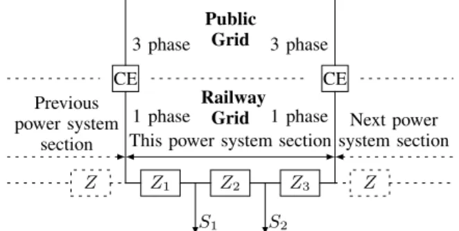
RPSS:s are by practical reasons rarely three-phase, but either single phase AC or DC systems. The AC systems are either operated at the same frequency as the public power grid or in a different frequency. If the frequency is different, it is normally a lower frequency. There are several different standards in voltage levels for the contact line for both the AC and the DC railway systems. The contact line delivers electricity to the trains, often as an overhead line called catenary. DC railway power supplies and AC power supplies with different frequency are similar in topologies, e.g. electric power has to be converted by power converters to be able to flow between the public grid and the railway grid. Doubly fed railway power supply system sections are connected as in Figure 1. The denotation Connecting Equipment (CE) is here used as a general name for the component that is either a converter station or a transformer connected to the three-phase public grid. AC railway grids with public frequency
simply have transformers instead of converter stations, using one or two of the public grid’s three phases. In order not to cause asymmetrical loading, the public-grid phases connected to the public-grid-frequency railway grid, are altered for each consecutive transformer station. Therefore, because of the 120◦phase angle difference, in contrast to the configuration of Figure 1, the public-grid-frequency railway is never fed from more than one CE at once. For a public-frequency railway system, the contact line would have been sectioned where Z2 is located in Figure 1. A more thorough overview of railway power supplies can be found in [8].
Z Z1 Z2 Z3 Z S1 S2 1 phase CE 3 phase 1 phase CE 3 phase Previous power system
section This power system section
Next power system section Public Grid Railway Grid
Fig. 1: A section of the railway power supply system, illus-trated as an electric circuit.
A. The Railway Grid Compared to the Public Grid
RPSS:s differ in some ways from public power systems. One special property is that the loads vary heavily over time, in a complex way, both in load size and load location [9]. Normally, the voltage levels are allowed to vary to a much greater extent in the RPSS, compared to the public one. Locomotives are designed to accept substantial voltage drops to a greater extent. The level of acceptance varies greatly between different models. The Swedish Rc locomotive will still be in operation for voltage drops of about 40 % [10].
Because of these great voltage variations, computing the load flows becomes more complicated, because a simple iterative algorithm is less likely to converge if the initial guess is too far from the true value [9]. Moreover, when electric nodes become too closely located, they have to be treated as one – otherwise the impedance matrices of the system would risk becoming close to singular [9]. In the general case, the problems can also be heavily nonlinear.
In order to be able to describe the variations in location and size of the loads, i.e. the trains, an RPSSOS software needs to consider a few details. An enough detailed simulation determines train locations, velocities, accelerations, contact line voltage levels, tractive efforts, and (if AC, active and reactive) power consumed. Inputs to such an RPSSOS are track inclinations, time tables, information about the power consumption of the electric motors of the trains and about the modeling of the CEs, impedance values for conductors, acceleration and speed-limits, running resistances, and weights of various trains.
B. CEs, Power Transmission, and How to Strengthen the Grid The CEs (”CE” in Figure 1) of a railway power supply system, may it be transformers, frequency converters, or rectifiers, normally have some kind of voltage regulation on their railway side terminals. Therefore the closer located each pair of CEs are, the smaller the voltage drops on the contact line will be for a given load. Indeed, for singly fed contact lines (which is the normal case with AC railways in public grid frequency) the voltages will drop even more for the same CE-pair distance. Singly fed sections can, in DC systems and low frequency AC systems, for example occur at contact line ends, sectioning of the contact line for security reasons, or in cases of CE outages.
In some setups, the RPSS have own generation, and also regeneration from braking trains. In the 1970s when power electronics improved, it became possible regenerating energy from DC motors to AC power supplies [11], a feature not only saving energy, but also increasing the maximal braking torque. When a positive net production of power is possible on the railway side of the CEs, it is good if the CEs also allow power to be sent in the other direction.
Power is transmitted through contact lines, and if available, also HV (High Voltage) transmission lines and the trans-formers connecting them to the contact line. The transmitting impedances, Zj, j ∈ {1, 2, 3}, are illustrated in Figure 1, as the total impedances seen by the locomotives.
The power grid can be strengthened by placing the CEs closer to each other or by reducing the per-meter impedances between the CEs. Per-meter impedances between CEs can be reduced in many ways. Impedances can in AC systems be reduced by e.g. switching out BT contact lines (Booster Transformer [12]–[14]) for AT (Auto Transformer [12]–[15]) ones. Sometimes AT systems are also called dual systems or 2xVL kV systems (where VL denotes the voltage level) [15]. There are also power-electronics based solutions with dual voltage contact line systems for DC railways [16]. Generally, conductors with less physical impedance, i.e. greater cross-sectional areas or conducting materials with lower impedance, can be used. Another alternative is to connect HV transmission lines in parallel (or meshed as well when the topography so allows) to the contact line system.
A transformer station for an HV transmission line is nor-mally cheaper to buy and operate than a converter station, so sometimes it might be better having a few strong converter sta-tions and a number of transformers spread out between them, instead of having many weaker converter stations densely distributed with just the contact line connecting them. By natural reasons, the need for specific railway HV lines is smaller for AC railway power supply systems using the public frequency.
C. Locomotives and Trains
When traffic is dense, fast, and/or the trains are heavy, the power consumption of the trains is high. Then, eventually, the contact line voltage levels will drop. The trains are in Figure 1 represented by the Sj, j∈ {1, 2}
For most locomotives the maximal possible tractive force is successively reduced for decreasing contact line voltage levels by on-locomotive controllers. This control is installed due to physical limitations and regulations. It is done in order to protect the engine from overloading, and possibly also for reducing the risk of voltage instability in the RPSS. This voltage level dependency varies in details between different train models [17]. Some train models also have a velocity dependency of the maximal tractive force.
If the tractive force minus the running resistance and the gravitational resistance is above zero, the train accelerates. If, conversely, the net tractive force is below zero, the train will decelerate. The running resistance is mainly caused by wind resistance and mechanical resistance of the train, and is normally modeled as a second order increasing polynomial function of train velocity. The gravitational resistance is caused by train weight and the slopes of the railway track.
From the three above paragraphs it can be seen that, if the traffic increases faster than the strengthening of the power grid, the trains will sooner or later be forced to travel either more sparsely, more slowly, on other routes, with reduced weights, or combinations of these, compared to what they used to.
The tractive power is the tractive force times the train velocity. There are normally electrical and mechanical power losses inside the train. The (active) electric power consumption of the train is the tractive power plus power losses inside the train. In AC systems, if any reactive power is consumed, it can be caused either by the motor type, or by the desire of the operator to raise or lower the contact line voltage.
The railway administrator can choose when, and what kind of investments to make in the railway power supply. However, all the times when there are demand for a traffic that the power supply would not cope with – the administrator has to consider that fact.
III. LITERATUREREVIEW OFVARIOUSLYRELATEDWORK
A. Fast estimators of the railway power supply
There are not so many existing methods for fast estimation of railway power supply system behavior known to the authors. The ones known are however discussed in the following.
Some efforts constructing an uncomplicated approximator, based on knowledge, intuition, and experience have been made in [18]. That paper presents a method to determine the minimum headway time, given the power system details as well as train data and the desired train velocity. In [18] however, the impacts of slopes are not considered, the power system is modeled very simple with assumptions not suitable for sparsely populated areas, and all the traffic is assumed to be homogeneous. Additionally, that approximator has not the same kind of input and output as required here.
In [5], the optimal point of coasting, considering the voltage drops and minimizing a trade-off between traveling times and energy consumption, is determined by using neural networks trained with simulation data as constraints in an optimization problem – quite similarly to what is done in this paper.
Neural networks are also in [19] used for estimating the voltage drops in the Bay Area Rapid Transit (BART) railway power system.
There is also a commercial software called OpenPowerNet available [20] that is a power system calculator connected to and communicating with Open Track (a railway operations simulator [21]) during simulation. The results from the power system calculations are considered in Open Track. The models of OpenPowerNet or Open Track are not available for the public. The approximator presented in this paper could be used similarly as OpenPowerNet, but as a part of an open source traffic planning software.
B. Decision Making or Planning for Dimensioning of Power Supply Systems
In [22], a beautiful algorithm for assigning locations of substations in a PRT (Personal Rapid Transit) system is presented. The objective is to minimize RPSS losses. It is not totally clear how the power consumptions are determined, and how they are smeared out into a so-called load power density on the power sections in [22]. The relation between voltage levels and tractive ability is not discussed.
In [23], RPSS:s are designed by making changes in the system setup and simulating once more until the system fulfils the demands of the designer. The more sophisticated methods for designing the power supply in [24], [25] are follow-ups to [23]. In [24], where substations are placed out and catenary setup is chosen to minimize the investment cost, a simplified DC model of an AC RPSS is used, using a set of operational scenarios where power consumption is assumed to be known instead of simulating all the train movements. Besides that, in [24], there are constraints for voltage levels, power transmission in lines, and capacities of substations. In [25], a genetic algorithm is presented for solving the problem presented in [24], the results are not far from optimal and the computation time is significantly decreased.
In contrast to TPSA presented in this paper, where the maximal tractive force is slowly dropping off, in [24], [25] voltages are either such that no trains can operate, or such that all trains operate perfectly. Moreover, only train traffic snapshots are studied, and the power system models are simplified.
In [26], treating the optimal expansion planning of trac-tion substatrac-tions for DC networks, nothing is said about the simulation times. There, however the models seem simplified. As an example, in [26], first, the train traffic is simulated disregarding the power system limitations. First after that is done, mechanical power needed is used in the load flow calculations, and investments are made such that the voltage levels never goes under a certain threshold value, and then low levels close to the threshold are associated with a cost. It is not totally clear how the planning procedure in [26] works. Moreover, in [26] only worst case scenarios are studied. Worst cases may happen quite rarely, and sometimes low voltage levels may be a price worth to pay. The research project which TPSA is a part of aims to approach problems like when or how often, and for which traffic situations it may be worth having an imperfect power system. The operation costs, e.g. from delays, and investment costs have to be balanced somehow in real life.
In [27], a tabu search algorithm is used for locating substa-tions and setting the rectifier firing angles in an optimal way for DC traction systems with fixed train headways. The op-timization in [27] is integrated with power system simulation instead of using snapshots in time. Tabu search is faster than standard optimization algorithms, but more approximative. Equal load sharing and minimizing energy usage are used as objectives. In [28], published before [27], the same objective is used, but the problem is solved with genetic algorithms. Here, the power consumption of trains is not voltage-level dependent and is determined in separate traffic simulations done before the optimization. In [27], the possible locations of substations are predefined, and not available on a continuous interval. The substations can be either regenerating or not.
In [29], the planning of where and when to invest in trans-formers feeding a DC RPSS is described. The transtrans-formers should be able to cope with the annual peak demand, and the investments and power losses are minimized. Simulink is used to determine train power consumption at each time snapshot. Power losses and investment costs in combination are minimized. Modeling details are however not presented in [29]. Still, the relation between maximal traction effort and voltage levels are explicitly pointed out in [29], which is the main focus in the TPSA presented in this paper.
In the, for the field early paper [6], nomographs are created by the use of simple power system models representing train traffic snapshots in time. These nomographs are supposed to be used as a hands-on support for engineers making decisions of where to locate railway power system substations.
In [30], the locations and sizes of harmonic filters are determined with the subject of reducing harmonic distortion in the railway power system.
C. Railway Power Supply System Operations Simulators There exist a number of publications about RPSSOS of dif-ferent kinds. Besides those, there also exist some commercial software – where, normally, the modeling documentation is not available for the public.
1) Commercial: The software originally developed by ABB
as SIMTRAC, nowadays marketed by Balfour Betty Rail as TracFeed Simulation [31], [32] is still developed in Sweden by STRI. The program is used by e.g. the Norwegian and the Swedish railway authorities and some subway companies.
The by Siemens developed Sitras Sidytrac [33] is used internally in the Siemens corporate group.
ELBASTOOLS from the manufacturer ELBAS including SINANET (for DC traction), WEBANET (for AC traction), and IMAFEB/ELEFEB that is suitable to the calculation of effective overhead line impedances of AC railways as well as the magnetic and electric field distribution at cross sections around the contact and transmission lines [34].
The µ-PAS, ZFS software from Prolitec AG, also exists as well as the software package Faber from Enotrac AG.
2) Academic: The simulation software TPSS (Train Power
System Simulator), considering the interaction between the train traffic and the railway power supply system, is based upon consecutive load flows, calculated in discretized time.
In TPSS, the trains consider running resistance, slopes and gravity, and the limited tractive effort of train motors de-pending on low contact line voltages. The simulator also allows arbitrary CE models and considers various reactive power consumption schemes, often heavily nonlinear. TPSS is presented in detail in the full report [2], whereas some modifications and improvements are presented in [35]. In [36] TPSS was compared with the commercial software TracFeed Simulation [31], [32], and the relevant results were correlated between the programs.
In [37], a very early presented RPSSOS for DC rapid-transit railways, containing electric models considering voltage drop impacts on tractive ability, is presented.
One comparatively detailed 50 Hz RPSSOS working in discretized time is presented in [23], also considering phase imbalances in the public grid. All contact line voltages in [23] has to lie within a certain range. Other 50 Hz simulators are presented in [38], [39].
DC RPSS, subways in particular, including the intercon-nected supplying AC system has been modeled and studied in [40]. In the train models, the tractive capacity and the load of the trains are assumed to be independent of the state of the RPSS. The train distribution system and the transmission system are separated in the power flow computations, as are the conductor and rail impedances in the modeling. Similar modeling to the one found in [40] is presented in [41], but there the modeled DC RPSS is the Dutch public railway. The DC RPSSOS used in [27], uses predefined load locations determined by a train traffic simulation excepting the power system.
The AC and DC load flow calculations in [29] are done sep-arately, first the DC railway load flow, then the AC supporting system, where the substations are modeled as fixed loads. In [42], the power flow between AC and DC is unified.
Different computation techniques exploiting the matrix spar-sity for load flow in DC railways are discussed and presented in [43]–[45]. Also higher voltage RPSS have been studied [46]. In [47], harmonics in RPSS have been studied.
D. Lectures and field overviews
The broad lecture on electric railway systems, [8], explains most of today’s RPSS standards and their technical, historical, and economical respective backgrounds.
In [48] different RPSS and their standards are explained – with a focus on various DC systems and the 25 kV 50 Hz system.
For another more general review (including different RPSS and other issues) of electric railway traction, please refer to [12], [49]–[54].
In [13], a brief but informative description of the Swedish RPSS can be found.
E. Other railway power system research
There are many published articles focusing on details of the RPSS. For dimensioning purposes however, it is enough keeping the steady state voltage levels as well as having capacity enough in converter or transformer stations. In [55],
the rail impedance nonlinear dependency on frequencies is studied. Also in [56], [57] transient frequency dependencies of impedances are studied.
In [58], a detailed study of the crosstalk between adjacent railways tracks considering signalling and electromagnetic compatibility can be found. Magnetically induced contact line voltages are studied in [59].
In [60], the possibility to control substations for DC RPSS with thyristors in order to share the loads between the substa-tions is treated.
Some articles consider the RPSS, whereas they keep focus on other things. In [61], instead of power supply investments, railway track investments are discussed, but the RPSS is also considered to some extent.
IV. THEAPPROXIMATOR
A. Power System Sectioning
1) Assuming the CEs can be Treated as Infinite Buses: Since the voltages normally are controlled at the railway side terminals of the CEs, it is in this paper assumed that the CEs can be approximated as infinite buses. That leads to a separation of the railway power system into many isolated and independent power system sections, whose borders are either CEs or simply the ends of the contact line.
2) Justification and Consequence of the Assumption: In
[62], a simplification similar to the one just presented can be found. There, a train is assumed to consume power only from the feeder units right in front of, and right behind it. In [62], ”feeder unit” means either a CE or a connection to an HV transmission line.
The power system sectioning assumption is an essential part of the TPSA model presented here. Its main benefit comes when considering the intended usage of TPSA. TPSA can, now that the power system has been split up into small pieces, easily be implemented as an optimization problem constraint. Such a constraint describes any traction power system section. The same constraint can even represent completely different neural networks. That property is of great value, as will be seen in Section IV-B. The separation of the RPSS into pieces makes the neural networks modeling more reviewable.
In [22], a similar sectioning of the power supply system is made. The motivation is however different, and a bit more complex.
3) Discussion about the Assumption: This is in most cases
valid, since the states of the neighboring power sections nor-mally do not affect the state of the studied section significantly. In rare cases, like when the traffic is very unevenly spread over the power sections and if the CE capacities in the studied power section are comparatively weak, power may have to be taken from neighboring sections. With, e.g. the presence of an HV transmission line, the power sections become somewhat less isolated and independent.
Last, but not least, the possible accuracy losses can be compensated for afterwards by different means.
B. Discrete TPSA Inputs Selecting which Neural Network to Use
1) Model: All inputs to the neural-networks-based
approx-imator TPSA are not neural network inputs. There are a few discrete variables that determine which of the available neural networks that should be activated.
The neural networks are only trained with inputs and outputs that can be regarded as continuous variables, i.e., ”remaining inputs” in Figure 2. The remaining inputs are presented in Section IV-C.
In Figure 2, to illustrate, the two binary variables ̺ and η tells which of four available neural networks to be activated.
S el ec to r TPSA outputs TPSA inputs AT ̺catenary HV η Remaining inputs TPSA NN #1 AT NN #2 AT+HV NN #3 BT NN #4 BT+HV
Fig. 2: For AT and BT contact line types, which can be either connected to or without an HV transmission line, there are four separate possible neural networks (NN).
The discrete TPSA inputs are listed in the following. a) The binary variable, ̺, tells whether or not the power
system is equipped with an AT contact line system. If not, a BT contact line system is assumed. For DC systems, AT contact line system means a dual voltage system like in [16], and not AT means a normal DC system. b) The binary variable, η, tells if there are HV transmission
lines available or not.
2) Motivation: The separation into different neural
net-works is motivated by the fact that backpropagation [63], [64] networks are not optimal for discrete classifying variables. Backpropagation networks are mainly intended to be used as approximators of smooth functions.
The choices of discrete inputs are motivated in the following list.
a) Gives information about the distance-dependent impedances of the contact line system.
b) Gives information about the distance-dependent impedances between trains and CEs.
3) Discussion and Possible Future Work: Indirectly, in the
model, it has been assumed that each power section has only one kind of contact line technology type (AT or BT, respectively). In real life, it happens, but is not very common that the contact line technology types change within the power sections. A future TPSA could include a method of managing this issue.
More discrete inputs than ρ and η might be needed in the future. To e.g. determine whether a power system section is doubly fed or singly fed is of importance for the strength of the section.
In the numerical example of this paper, all contact lines are doubly fed, so such input is not needed here. The numerical
example is from a 16.7 Hz railway but it could – considering only the topology of the power grid and the principal behavior of the trains, i.e. disregarding the exact figures in km/h, minutes, etc. – also represent a DC railway system.
C. Remaining TPSA Inputs, Continuous Inputs to the Neural Network
1) Model: The remaining TPSA inputs follow in the below
list.
a) The length of the power system section. That means the distance between a pair of CEs or between a CE and the end of the contact line.
b) The average inclination of the track between the power system section borders. The sign of the inclination is defined as it would have been experienced by the added
train traveling all through the power system section.
c) The standard deviation of the inclination, in the power system section
d) The average number of (other) trains, γ, on the power system section. The average number of trains is here defined as the total already scheduled train traffic time in the power system section before adding train rN, during the time window when the added train traffics the section, divided by the length of the same time window.
e) The average velocity of the other trains in the power system section in the above time interval, vo. The average velocity is measured only when trains are moving.
2) Motivation: TPSA assumes a scheduling process, where
an added train (train rN) to the time table should not affect the state of the power system in such a way that the trains already scheduled (subset of trains r1, r2, ..., rN −1) in the same power system section at the same time (as train rN) should have to be rescheduled due to lost tractive capacity. The maximal speed of the added train can be seen as a measure of the traffic performance.
The idea is to describe the already scheduled trains in a lumped-together manner to the neural network of TPSA. There are two main reasons for this, of which the first one is the most important.
The first one is to keep the number of inputs to the neural network small. Many inputs increase the degrees of freedom. Like with polynomial data fitting, a network with many degrees of freedom demands a tremendous number of training cases in order to become reliable and generalizable. Training [63] means the iterative adjustment of the neural network parameters such that the network behaves as desired. The second one is to have a constant number of inputs – regardless of the number of trains in the power section. There is no obvious theoretical upper bound on train density, so how many inputs that would be enough if treating all trains as individuals, is not obvious. Moreover, with the model suggested, assigning which train that should belong to which input, will not have to be an issue.
The inputs are motivated in the following list.
a) The distance gives information of the power system impedance.
b) The average inclination gives information of the net potential energy consumed by the trains traveling within the section (more power consumed), but also on the aggregated running resistance for the studied train (more power consumed, and may also directly influence the speed).
c) The standard deviation of the inclination is needed be-cause the average inclination is not informative enough. The average inclination would for example equal zero for both flat ground as well as for a steep uphill slope half the section and an equally steep downhill slope in the remaining half. The standard deviation is a measure of how much the inclinations fluctuate, which will influence the consumed electric power of the trains.
d) The number of trains is important because the more trains, the greater the need for electricity.
e) Not only the number of trains on a section determines their power consumption, but also their on-average ve-locities.
3) Discussion and Possible Future Improvements: In this
paper, the model is restricted to one type of trains traveling in one direction. When there are trains with different mechanical and electrical properties in traffic, it might be necessary to have inputs for each train type, probably including the running resistance coefficients (see e.g. [65]) of the train type. Bidirectional traffic might also cause a need for extra inputs. When TPSA is used in a time tabling program, inputs d) and e) in Section IV-C are sometimes depending on the output. The added trains traveling time is bounded below by, and therefore depending on, the maximal velocity, i.e. the output. At the same time the average number of trains, input d), and the average velocities, input e), are calculated by the use of the traveling time of the added train.
A sixth continuous input that describes the reduction of impedance by the transformers inside the section when there is an HV line present could be of need to be implemented in the future. This input will probably not be integer, because in reality the transformers are rarely evenly distributed. A contin-uous variable describing how well distributed the transformers are, is thereby expected to be needed.
Ohmic descriptions of power lines would introduce the ability of TPSA to judge between different kinds of BT and AT contact lines as well as HV lines. These have different per-km impedances.
D. Output: The Fastest Possible Average Velocity of an Added Train
1) Model: The output is the maximal possible on-average
velocity of the added train, see Section IV-C.2.
2) Motivation: When creating a train time table, the
sched-uler needs to know the maximal possible on-average train velocity for each train. The reason why only average velocities are used is that it is common to model train time table planning programs [66]–[71] such that you know when and where the trains starts and stops – but nothing more. Obviously, only average train velocities can be used, and variations of the velocity between two train stops has to be unconsidered.
The added train is by TPSA treated as an individual because there is no other way determining the maximal speed for each train.
3) Discussion: The output of TPSA tells at which maximal
average velocity, vrN
max, the added train is allowed to travel, for each given power system section, with a given track topogra-phy, and given that the then and there already scheduled traffic does not accept to consist of less than on-average γ individual trains traveling in at least the average velocity vo. This is, due to the lumping-together of the other trains, the closest to the desired goal of not rescheduling the existing traffic at all we can come.
In time tabling programs (except e.g. the commercial pro-gram OpenPowerNet [20]) the maximal velocities are fixed. In reality however, they are not. Voltage drops cause trains to go slower, as explained in Sections I-B, II-C. In order to simplify, instead of doing time tabling with variable speed-limits, a cost can be assigned to trains with reduced speed, as in [7].
E. Summary
The choices of aggregated inputs and output are adjusted for the kind of information that one can expect to be available from both detailed RPSSOS/measurements and train time table planning software. This does of course reduce the available choices for the design of the inputs and the output of the TPSA. Simulations/measurements are supposed to be used for the training data of the neural networks of the approximator. Simulators need to model the voltage drops at the contact lines, and their impact on the maximal train tractive force, to be useful for TPSA training.
V. NUMERICALEXAMPLE
A. Introduction
Two different neural network models are suggested and evaluated, both based on the output and inputs presented in Sections IV-B, IV-C and IV-D.
The first model, M1, is a nonlinear neural network with two layers, expected to be enough for the purpose. The first (hidden) layer has tanh (tansig) transfer functions, a choice made based upon empiricism. The second (output) layer has a linear transfer function. There are five inputs, c.f. Section IV-C, and one output, c.f. Section IV-D. Nonlinear artificial neural networks, like M1, can be used as general function approximators, given a sufficient number of neurons in the hidden layer(s) [72].
The second model, M2, is a linear neural network. And since model M2 is linear, adding more layers than the input and the output layers adds nothing to the neural network performance. The motivation for testing a linear model at all is explained by the intended use of TPSA in optimization programs. The accuracies of the two models are compared and evaluated in Section V-D.2.
B. Training of the Neural Networks
In both M1 and M2, the aggregated input and output data sets are normalized to lie in the interval [−1, 1] by simple scaling before training and testing the approximators.
Training is essentially a method of determining the values of the neural network parameters (weights and biases) such that the network behaves as desired. Commonly, this means that mean square of the estimation error of the network output is minimized, which is the case also here. Normally, the maximal number of iterations (epochs) is limited by the user and in this paper, the maximal number is set to one thousand for both M1 and M2.
Model M1is trained by the trainbr (Bayesian regulariza-tion backpropagaregulariza-tion [73]) algorithm (of Matlab’s Neural Net-work Toolbox) with an error goal of10−5. The default training algorithm trainlm (Levenberg-Marquardt backpropagation [74]) has also been tried out, and in general it works as fine as trainbr. In some rare cases however, for the specific sim-ulation data used, trainlm tends to overlearn the presented data rather than extracting the important trends from it. Model M2is trained by the trainb (batch learning [75]) algorithm (of Matlab’s Neural Network Toolbox).
C. The Used Training Data
1) Introduction: The training data used for TPSA in this
example are extracted out of TPSS [2] simulations. The sim-ulations represent variations in traffic, length, and the power system technology of a typical Swedish RPSS section.
However, the training data could as well have been created from measurements and be representing different types of railway power systems than the one used here.
As a consequence of the Swedish-like model, the CEs, c.f. Figure 1, are here converter stations, and the high voltage line is of the in Sweden most common 132 kV type. Since the Swedish system is AC, the contact lines can be of either AT or BT types. Contact lines and transmission lines are in Figure 1 represented by impedances.
2) Power System Infrastructure Used: In the simulations,
each power section has the same contact line technology type (AT or BT, respectively) all over it, a consequence of the TPSA modeling. The simulated traffic is unidirectional.
In the Swedish railway power supply system, the defacto nominal contact line voltage level is 16.5 kV, however it is officially said to be a 10 % over voltage in a 15 kV system. The voltage angles at the converter station terminals are completely determined (although quite nonlinearly) by the voltage levels, and the active and reactive power flows in and out (if possible and allowed) of the terminals of the converter station [76]. And converter stations are injecting more power to the railway, the more installed power there is in the station compared to its neighboring stations.
The converter stations, the CEs in Figure 1, at both ends of each power system section are in the simulations equipped with six 10 MVA converters (Q48/Q49 [76]) each, i.e. 120 MVA in total. That guarantees that the amounts of installed apparent power will not be a limiting factor in the simulations studied. Assuming about 4 MW for each train, and an average velocity of 100 km/h on a 160 km section and a headway, i.e. a train departure time distance, of 6 minutes gives around 65 MW in total – allowing some reactive power consumption and transmission losses.
It is here worth pointing out that in [2] it has been shown that the train velocities are in practice not dependent on the mutual distributions of apparent power capacity between a pair of converter stations, so these simulation results used for creating the training data are representative for all different variations of converter station capacities.
In the simulations with an HV transmission line present, the number of transformers connecting the transmission line to the contact line is set to three in all cases studied. This means that there are five transformers in total, three out on the track, and one connected to each converter station. The transformers are evenly distributed along the track.
3) Information About Trains Used: Since the model
pre-sented in Section IV assumed only one kind of trains, the simulations used one kind of trains as well – Rc4 [10] in this case.
Trains start and stop at the power section borders in the simulations. Since all systems here are double-fed, this means that a train starts at a converter station location and also stops at one. The term ”double-fed” means here that a contact line is fed with power from not just one of its ends, but from both. The speed-limit on the simulated track is in the simulations set as high as 150 km/h. That speed is for Rc4 locomotives a limiting constraint only in very steep downhill situations. There are in the simulations no train-individual speed-limits. All trains try to go as fast as possible in the TPSS simulations, i.e., as fast as the track speed-limits and the physical con-straints of the railway in total allows. In the simulations used for creating the TPSA training data, the continually maximal-tractive-force curve from [10] was used. A higher tractive force than the continually maximal-tractive-force may sometimes be used for shorter times without damaging the motors. However, the tractive force differs between the continually and the short-time curves mainly for low velocities. Thereby, any maximal-force curve, results in similar simulation results, as another maximal-force curve would do, when there are not so many frequent stops and accelerations of the trains.
4) Description of Training Data Before Aggregation: A
train has in a TPSS simulation been followed. An example of the world as it is seen by that train is visualized and presented in Figure 3. This is done in order to give the reader a picture of the behavior of the railway power system and what kind of simulator TPSS is.
At the same time interval, the summed active and reactive power consumptions of all trains in the same power section are plotted, together with the active and reactive power injections from the two converter stations, in Figure 4. All plots in Figure 4 are in per unit, with base power 5 MVA.
In that simulation, the power section length was 160 km on a BT system with HV line and the headway was 6 minutes. The velocity of the train, v, is in Figure 3 scaled down by a factor of 160 km/h. During this particular simulation, the studied trains speed varies between 151 km/h downhill and 89 km/h uphill. Additionally, Figure 3 presents the trains consumed active power, PD, reactive power, QD, and the contact line voltage, U , all expressed in p.u., where the used base power Sb is set to 5 MVA and the base voltage level Ub is the same as the nominal contact line voltage level, i.e.,
0 20 40 60 80 100 120 140 160 −0.4 −0.2 0 0.2 0.4 0.6 0.8 1 km v 160 km/h U 16.5 kV PD 5 MW QD 5 MVAr ι·1000 20 + 0.5 ι = 0 −radiansθ
Fig. 3: An example of the mechanical and electrical states of a train traveling through a section of the railway electric power supply system.
16.5 kV. The contact line voltage phase angles are in Figure 3 presented with opposite sign, i.e,−θ, and expressed in radians. Finally, the inclinations of the railway track, ι, are plotted in Figure 3, scaled in such a way that the range -10 h (per mille) to 10 h is depicted in the range 0 to 1.
In order to save TPSS computation time when simulating a certain headway of the traffic, trains are evenly distributed along the track assuming that the trains have been going at maximally allowed speed all the time – disregarding possible slopes, air resistances, or weaknesses in the power supply. These trains are so to say, the initial condition of the simula-tion. This means that simulation results of the added train will be obtained all through the simulation. To study the filling-up of the track from a no-traffic situation is not of interest in this study. If filling the track up by simulations than this maximal-speed-assumed situation, the trains should have become slightly denser distributed along the track, since the velocities are reduced from time to time.
In the initial conditions, the distributed trains, assumed to already be in traffic, have velocities set to the maximal value. After the simulation has started however, the trains distributed along the track with predefined initial velocities will follow the same electrical and mechanical laws of nature as the other trains. Therefore, the number of trains within the section will slightly increase when their velocities goes down from ideal to real values. This fact explain the increasing trend of the curves in Figure 4. In the simulations, a steady-state of the train traffic is never reached.
10 20 30 40 50 60 70 80 −5 0 5 10 minutes ΣPD ΣQD Converter station 1, PG Converter station 2, PG Converter station 1, QG Converter station 2, QG
Fig. 4: An example connected to the one in Figure 3, the plot is for the same time window, and visualizes the total power consumption in the section and the power injected from the converter stations as functions of time.
5) The 400 training cases: In the numerical example, 400
different simulation results have been used, 100 for each neural network to train. There are four separate neural networks, one for BT-type contact lines, one for AT-type contact lines, one for BT with HV transmission line, and finally one for AT with HV transmission line – as described in Figure 2.
These 100 cases (for each power system type) consists of ten different power section lengths: 30, 57, 80, 98, 114, 127, 138, 146, 154, and 160 km. The simulations are done on the same rail section, with the inclination curve shown in Figure 3, where the first converter station is fixed in location at 0 km, and the other one is moved as the power section length changes. These different power section lengths are in turn combined with ten different headway times of: 6, 8, 10, 13, 17, 22, 28, 36, 46, and 60 minutes.
The case studies here have been selected to create significant voltage drops. Therefore, heavy trains with comparatively high running resistance have been used. Then, the main reason for not simulating headways shorter than 6 minutes is that with the heavy trains studied here, the voltage drops would be too great for BT-type contact lines in combination with long power sections. Moreover, the set of training data was purposely kept small to show the learning ability of the neural network. For lighter trains, and the same power supply, much shorter headways could be simulated, resulting in moderate voltage drops.
The power section lengths quite obviously make out input a) in Section IV-C. In this study, the variations in power section lengths also give rise to variations in inputs b) and c) in Section IV-C. That relation exists mainly because all simulations are here made on the same track. The headway times primarily gives rise to variations in input d) of Section IV-C, but also to e), to some extent.
D. Evaluation of the TPSA Performance
2 4 6 8 10 0 0.02 0.04 0.06 0.08 0.1 0.12 E rr o r Number of neurons
(a) AT-type contact lines and no HV lines
2 4 6 8 10 0 0.02 0.04 0.06 0.08 0.1 0.12 E rr o r Number of neurons
(b) BT-type contact lines and no HV lines
Fig. 5: A study of the average mean square errors on the training and testing sets as a function of the number of hidden neurons. Dash-dotted line denotes the training set curve and solid line denotes the test set curve.
1) Size of TPSA:s Neural Networks in the M1 Nonlinear
Model: As rule of thumb, during the evaluation of the neural
network, two thirds of the data set may be used for training the neural network, whereas the remaining third may be used for testing. That proportion is used when evaluating which neural network size to chose in this paper as well.
By studying the average mean square approximation errors for one to ten neurons in the hidden layer, an idea of the right size of the neural network can be made. The average was calculated for 20 different random choices of training and testing sets. The results of the study are presented in Figure 5. In Figure 5b, it is shown that the errors in the testing set starts to increase for more than four hidden neurons for the BT contact line system. That phenomenon is due to overlearning and thereby lost generalization ability. In the three other, stronger, power systems, it is much easier predicting the maximal possible velocity since its values do not fall as fast as for pure BT systems. For different power system types, the maximal velocity of an added train as a function of the surrounding train traffic in the power section are illustrated in Figure 8 further down in Section V-E.2.
The number of hidden neurons for model M1was set to4, not only for pure BT, but for all types. The reason is that, the testing set errors are not decreasing for an increasing number of hidden neurons. The results for HV line together with
BT-type contact lines as well as HV line with AT-BT-type contact lines look similar to the pure AT results in Figure 5a. Too many degrees of freedom when fitting a function to measurements normally increase the variation of the function in an unwanted way.
2) Comparing the Nonlinear Model M1 and the Linear
Model M2: This part of the evaluation of the TPSA
perfor-mance concerns a comparison of the accuracies of the two neural network models dealt with in this paper, the linear neural network, M2, and the nonlinear neural network, M1. Here, like in Section V-D.1 the comparison is made for both training and testing sets, and the results are averaged of 20 randomly chosen training and testing sets.
TABLE I: The approximation errors for the four different neural networks for model M1
Training Set BT AT BT AT HV HV No HV No HV 3 .78·10−3 6.04·10−3 6.35·10−3 8.17·10−3 Testing Set BT AT BT AT HV HV No HV No HV 7 .06·10−3 1.37·10−2 3.95·10−2 1.23·10−2
The averaged mean square approximation errors for network M1are presented in Table I. The errors for network M2where about ten times the size of the errors of M1. The computer time needed for execution of minor neural networks like these ones is negligible.
However, M2, turned out to be of no use. When extending the training data set to the entire data set, the training algorithm of M2did not converge. To use all 100 cases for training of a network can be seen as there existed 50 additional simulation cases that the neural network should be tested against later. Therefore, M2is rejected as model candidate and will not be considered in the remainder of this paper.
3) Extra Evaluation of M1: The performance of the M1
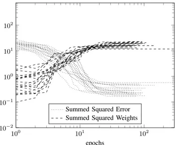
training are described in detail, for the 20 different, and randomly chosen training sets in Figures 6 and 7. In Figure 6, the summed squared weights and the summed squared errors of the neural network are plotted for each epoch. The figure shows that all 20 randomly chosen training sets converge well in training. That is seen by the fact that the weights converge in value, and the error go down to a level where they cannot be reduced more – and that is where the algorithm converges. The training times in seconds, are shown in Figure 7 for the 20 different simulations. In the same plot, the number of needed iterations/epochs, divided by 100, are also presented. The training times are in themselves not so interesting for the intended application of TPSA, since TPSA will ideally just be trained once, and then just used.
The weights in the hidden layer, wk,l, where k stands for input, and l for neuron number have also been analyzed. By summing the squares of the weights, over the neurons, and taking the square root of that remaining vector, an idea of the
100 101 102 10−2 10−1 100 101 102 epochs
Summed Squared Error Summed Squared Weights
Fig. 6: Convergence graph of the summed square weight factors and the summed squared error for each iteration/epoch. The plots are for the 20 different and randomly chosen distributions of training and testing sets. The error graphs are, naturally, for the training set. The plot represents the neural network for BT-type contact line only. The graphs look similarly for the other kinds of power supply.
2 4 6 8 10 12 14 16 18 20 0 2 4 6 8 simulations Training Times (s) Epochs 100
Fig. 7: In the above graphs, the learning times in seconds are plotted with the number of needed iterations/epochs for the training algorithm to converge. The graph is for pure BT and its corresponding neural network. The graphs for the contact-line-only graphs looked about the same, and those with an HV transmission line present showed about the double in number of epochs and training times as the contact-line-only graphs.
importance of each input can be obtained,
s X l (wkl) 2 = 0.94096 0.80359 1.3138 0.83884 0.43741 (1)
and the standard deviation of the inclinations seems to be the most important input, whereas the speed of the existing traffic is the least important. However, for a different, and especially greater data set the results could be altered.
E. An illustration of TPSA in Practice; a Validation of TPSA Interpolating and Extrapolating the by TPSS Generated Data
1) Prerequisites for the Detailed Study: Up to here, the
design of the neural networks of TPSA has been determined, and the evaluation of TPSA has been done on a macroscopic level. Here, it is time to study details, i.e. the maximal possible velocity of the added train as a function of already existing traffic on the railway section.
In order to make the output of TPSA a function of one variable and thereby easier to illustrate and visualize, input e) in Section IV-C has been omitted. This is implicitly based on the assumption that knowing input d), γ, means also knowing input e), vo. When the train traffic is homogeneous it is close to the truth. Here, ”homogeneous” means that all trains are: of the same kind, aiming to drive in the same velocity, and evenly distributed in time and space. After doing that, the neural networks of TPSA has been retrained with inputs a)–d). This leaves four remaining inputs. All simulations are done on the same track profile, and inputs b) and c) of Section IV-C are completely determined by input a) in Section IV-C. This, together with keeping a) constant in the plots, gives one independent parameter per plot – as was the intention.
From Section V-E on, all the 400 cases of simulation data, are used for neural network training, in order to maximize the TPSA performance. In this study, besides the 400 cases, one extra training case has been added for each of the four networks and each of the ten power section lengths simulated, i.e. 40 extra cases. This is done because it became obvious that the available simulation data includes too few cases with really dense traffic for short power sections and for power sections with an HV line. When lacking data describing really dense traffic, it is very hard for TPSA to catch the strictly decreasing behavior of the added trains maximal velocity for an increased number of other trains. The added data says that the maximal velocity of the added train, vrN
max, should be 0 km/h when there already are 50 scheduled trains, γ. These figures are chosen in a way to force down the asymptotes of the vrN
max curves when traffic is high.
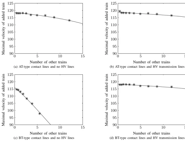
2) The Detailed TPSA Study: In Figure 8, the power section
length is 160 km for all plots. In that figure, TPSA interpolates and extrapolates vrN
max as a function of γ. The four subplots, Figures 8a–8d represent each of the four different power system technologies giving rise to different neural networks as explained in Section IV-B. As one can expect, and as Figures 8a–8d confirm, the pure BT system is the one that creates the greatest drop in maximal train velocity for an increased number of trains on a section.
The longest power section where the TPSS calculations converged for all simulated headway times, also for the pure BT system, is 114 km, c.f. Figure 9a. For 160 km power sections, pure BT simulations converged for headway times of thirteen minutes and longer. For a power section of 30 km,
0 5 10 15 90 95 100 105 110 115 120 125
Number of other trains
M ax im al v el o ci ty o f ad d ed tr ai n
(a) BT-type contact lines and no HV transmission lines, the inter-converter station distance is 114 km
0 5 10 15 90 95 100 105 110 115 120 125
Number of other trains
M ax im al v el o ci ty o f ad d ed tr ai n
(b) BT-type contact lines and no HV transmission lines, the inter-converter station distance is 30 km
Fig. 9: An illustration how vrN
max depends upon γ. The *s are TPSS results whereas the solid lines are TPSA outputs.
the velocities are, even for pure BT, quite unaffected by the densest traffic simulated, c.f. Figure 9b.
For really short power sections, vrN
maxis comparatively low. For a lone studied train, vrN
max is 105 km/h for a 30 km power section, c.f. Figure 9b, whereas for a 114 km power section, vrN
max goes up to 115 km/h, c.f. Figure 9a. This can be explained by the fact that for short traveled distances the time it takes to accelerate the trains makes out a greater proportion of the total traveling time. Power section lengths of 80 km resulted in the highest train speeds for pure BT (117 km/h) and AT (119 km/h). The impedances grow too big for greater power sections – resulting in voltage drops and reduced tractive capacity.
VI. CONCLUSION ANDSUMMARY
In Section I the field of railway power supply dimensioning was introduced, and the importance of this paper was mo-tivated. A literature review of relevance for this paper was presented in Section III. In Section II, railway power supply system models was discussed as well as a comparison between public grids and railway grids.
A suggestion to a new fast method, TPSA, of estimating the power system impact on traffic performance, has been presented in Section IV. The function approximator uses aggregated parametric values for inputs as well as for output.
0 5 10 15 90 95 100 105 110 115 120 125
Number of other trains
M ax im al v el o ci ty o f ad d ed tr ai n
(a) AT-type contact lines and no HV lines
0 5 10 15 90 95 100 105 110 115 120 125
Number of other trains
M ax im al v el o ci ty o f ad d ed tr ai n
(b) AT-type contact lines and HV transmission lines
0 5 10 15 90 95 100 105 110 115 120 125
Number of other trains
M ax im al v el o ci ty o f ad d ed tr ai n
(c) BT-type contact lines and no HV lines
0 5 10 15 90 95 100 105 110 115 120 125
Number of other trains
M ax im al v el o ci ty o f ad d ed tr ai n
(d) BT-type contact lines and HV transmission lines
Fig. 8: An illustration how vrN
max depends upon γ when the inter-converter station distance is 160 km. The *s are TPSS results whereas the solid lines are TPSA outputs.
The proposed method is general in many ways. There are no indications that TPSA should not be possible to apply to other kinds of doubly fed RPSS:s (including doubly fed DC RPSS:s), than those used in the numeric example. TPSA has been applied to a small specific railway power supply system in order to confirm its usability.
TPSA was evaluated in Section V, and a comparison between the two initially suggested approximator models M1 and M2 was presented, and M2 was rejected as an alternative during the study.
For M1, one hidden neural layer was assumed to be enough in all of the four neural networks. In that layer, four neuron were used. That choice worked fine with the data sets used, and not so many inputs. An example of the simulation results used were presented in graphs. Simulation data from 400 different, but systematically chosen cases were after proper aggregation used as TPSA training data.
Finally, in order to visualize the TPSS data trends, and how TPSA manages to adapt to them, a number of graphs in Figures 8 and 9 were presented and their content was discussed in detail in Section V-E.
It is obvious that TPSA manages to give reliable results in a fast way for given power system setups and traffic intensities.
VII. DISCUSSIONS ANDFUTUREWORK
The results presented in this paper, show that by making many simulations (or detailed measurements) and studying
the results – a feeling can be acquired for what is important regarding the railway power supply system and its interaction with the train traffic. Owing to that, the here presented approximator could be made.
Improvements in TPSA can be made in the sense that for more all-embracing data sets, different inputs would be possible, see the discussions in Sections IV-B.3 and IV-C.3.
Other future work are naturally to apply TPSA in investment decision programs, like in [7] but improved. TPSA can also be applied in traffic planning programs.
REFERENCES
[1] L. Abrahamsson and L. S¨oder, “Fast Calculation of the Dimensioning Factors of the Railway Power Supply System,” in Computational
Methods and Experimental Measurements, vol. XIII, Prague, The Czech Republic, Jul. 2007, pp. 85–96. [Online]. Available: http://www.ee.kth. se/php/modules/publications/reports/2007/IR-EE-ES 2007 019.pdf [2] L. Abrahamsson, “Railway Power Supply Models and Methods for
Long-term Investment Analysis,” Royal Institute of Technology (KTH), Stockholm, Sweden, Tech. Rep., 2008, Licentiate Thesis. [Online]. Available: http://kth.diva-portal.org/smash/get/diva2:117/FULLTEXT02 [3] L. Abrahamsson and L. S¨oder, “Fast estimation of the relation between aggregated train power system information and the power and energy converted,” in Universities Power Engineering Conference, 2008.
AU-PEC ’08. Australasian, Dec. 2008, pp. 1–6.
[4] S. Methner, “Multicriterial Optimization for Elecric Railway Systems (original title in German),” Dresden University of Technology, Tech. Rep.
[5] S. Acikbas and M. T. S¨oylemez, “Coasting point optimisation for mass rail transit lines using artificial neural networks and genetic algorithms,”