The Impact of Trade Openness on Gross Domestic Product : A study of the Asian Financial Crisis

J

I

B

S

JÖNKÖPING UNIVERSITY

T h e I m p a c t o f Tr a d e O p e n n e s s

o n G r o s s D o m e s t i c P r o d u c t

A study of the Asian Financial Crisis

Bachelor thesis in Economics

Author: Alexander Severin (860407)

Elin Glommen Andersson (860405) Tutor: Associate Professor Scott Hacker

Acknowledgements

We would like to thank our tutors Associate Professor Scott Hacker and PhD. Candidate Hyunjoo Kim who have guided and advised us through this C-thesis.

Furthermore we want to thank our families and close ones who have supported us throughout this process.

January 2009, Jönköping, Sweden

Bachelor thesis in Economics

Title: Trade openness and the impact on the Gross Domestic

Product – A study of the Asian Financial Crisis

Authors: Alexander Severin

Elin Glommen Andersson

Tutor: Associate professor Scott Hacker

PhD. Candidate Hyunjoo Kim

Date: January 2009

Subject Asian Financial Crisis, trade openness and gross domestic prod-uct

Keywords Current Account Reversal, Trade openness, Gross Domestic Product, Financial Crisis

JEL Classifications: E01, E44, F32, G18

Abstract

This bachelor thesis in economics examines the Asian financial crisis - its impact on the countries in the region and how well they recovered financially. The countries that are tak-en into consideration are Japan, Indonesia, South Korea, Philippines, Thailand, Malaysia and Singapore. The variables used to explain the implications of the crisis are GDP, trade openness, unemployment and current account.

Descriptive statistics show that the most closed economy that was affected by a current ac-count reversal was also the hardest hit in terms of GDP. The statistics also show that all the countries under observation have recovered to their situation prior to the crisis in terms of GDP, but not in terms of the level of unemployment.

Two regressions that were performed showed the relation between trade openness and the effect of GDP after the crisis, and the relation of trade openness to growth after the crisis. The regressions show that the more closed an economy is the larger the effect of a crisis. At the same time these countries had the highest growth rates after the crisis and were also among the first to recover. Theoretical reasons for these results are given.

Table of Contents

1

Introduction ... 1

2

Background ... 3

3

Theory ... 7

3.1 The effect of trade openness on GDP ... 7

3.2 Current account reversal ... 8

4

Empirical Framework ... 9

4.1 Method and Hypothesis ... 9

5

Empirical Results ... 11

5.1 Unemployment ... 11

5.2 Gross Domestic Product ... 12

5.3 Current Account ... 14

5.4 The relation of the 1998 GDP drop to Openness ... 18

5.5 Openness of countries and growth ... 21

6

Conclusion ... 25

References ... 26

Appendix 1 ... 28

Appendix 2 ... 29

Appendix 3 ... 30

Appendix 4 ... 30

Appendix 5 ... 31

Appendix 6 ... 32

Appendix 7 ... 33

Appendix 8 ... 33

Appendix 9 ... 34

Appendix 10 ... 38

Figures

Figure 5.1.1. Unemployment after 1997 (1)...10

Figure 5.1.2. Unemployment after 1997 (2)...11

Figure 5.2.1. Change in log of GDP after 1997 (1)...12

Figure 5.2.2. Change in log of GDP after 1997 (2)...13

Figure 5.3.1. Current Account over average GDP (1)...14

Figure 5.3.2. Current Account over average GDP (2)...15

Figure 5.4.1. The change in GDP in 1998 in relation to openness...17

Figure 5.4.2. The change in GDP in 1998 in relation to openness without Japan...17

Figure 5.5.1. Openness in relation to the slope of average growth after 1997...20

Figure 5.5.2. Openness in relation to the slope of average growth after 1997 without Hong Kong or Japan...20

Tables

Table 5.4.1. Regression results summary for the change in GDP in 1998...19

1

Introduction

In today‟s modern history the most well known financial crisis of all time is the Wall Street crash of 1929 (oxford reference, 2008). This financial crisis spread across to most econo-mies around the world. Since then there has been a number of crises, amongst these are those in Russia, Latin America, South-East Asia and now recently the worldwide economic crisis. The frequency of financial crises seems to have been increasing during the last twenty years with major upsets in the economy across the world. The magnitude of each crisis has been altering in size with varying numbers of economies being affected, but one thing is for sure - a financial crisis never goes by unnoticed.

The term financial crisis is very broad and can be used in many situations. It is used when referring to a banking crisis, a recession, a stock market crash, a currency crisis and the bursting of a financial bubble. Thus it is not easy to define what a financial crisis entails. In the case of the Southeast Asian financial crisis it falls under the category of a currency cri-sis.

“A currency crisis occurs when investors flee from a currency en masse out of fear that it might be devalued. Currency crises are episodes characterized by sudden depreciations of the domestic cur-rency, large losses of foreign exchange reserves of the central bank, and (or) sharp hikes in domestic interest rates.” (Kaminsky, 2008)

There are often many reasons to why a currency crisis occurs and how large the magnitude of the crisis is. In the case of Southeast Asia the economic situation for each country is generally very similar, with the economies built on the same principles. The macroeco-nomic policies of these countries were very similar and the countries are closely linked through trade. When the crisis hit, originating in Thailand, it immediately spread to many trade partners, a phenomena known as the contagion effect.

In general the Asian economies are viewed as being very open in terms of trade. The level of trade openness varies between the countries, some are more open than others. To a large degree these countries are very dependant on trade in their GDP. Does the level of openness thus have an impact on the countries in Asia when the crisis occurred?

A financial crisis changes the course of history and has a large impact on the personal lives of people. The way in which governments run their economies determines the stability of a country‟s economy, the economy of their people and to what magnitude the country will be affected.

1.1 Purpose

The Asian financial crisis affected a lot of economies in Asia as well as other economies across the world. The aim of this paper is to analyse what effect the openness of each economy had on the gross domestic product and how long time it took for each country to recover after the Asian financial crisis.

1.2 Outline

The rest of this paper is organized as follows. Section 2 gives a brief background to the Asian financial crisis and previous research on that particular crisis. Section 3 gives a theo-retical base to the paper and the theory explaining the hypothesis. Section 4 consists of the

data collected and regression method, whilst section 5 is used to analyse this results. The last section 6 is the conclusion of the thesis, which is followed by a list of references.

2

Background

This section will provide information about the situation prior to the breakout of the fi-nancial crisis along with previous researches views on the cause of the crisis.

2.1 History

The Asian financial crisis originated with the fall of the Thai Baht on the 2nd _{of July 1997}

(Montes, 1998). As a direct consequence a number of countries associated with Thailand were affected by this. As found throughout the reading, the countries that were most af-fected in the crisis were:

1. Thailand 2. Malaysia 3. Indonesia 4. Philippines 5. South Korea 6. Hong Kong

The fall of the Thai Baht was what triggered the actual crisis, but there are so many other factors that play in when the actual crisis broke out. The Southeast Asian economies had been experiencing a very positive economic climate since the beginning of the 1990‟s. The interest rates overall in the Asian region were fairly high during the early 1990‟s up un-til the crisis hit in 1997. Thailand‟s interest rate ranged from 9.5% to 12.5% during 1989 to 1997, but by 1999 it had fallen to 4%. Other economies close to Thailand such as Indone-sia were also experiencing very high interest rates ranging from 8.82% up to 20% in 1997. The Philippines had similar experiences whilst Malaysia and Korea were looking at more typical numbers around 5%. Due to the high levels of interest, a lot of investors saw the opportunity to invest and in turn get a high rate of return on their investments. This also increased the economic climate with a lot of money inflow to the region‟s economies (In-ternational Financial Statistics Yearbook, 2000).

There are many explanations to the cause of the Asian financial crisis, according to Montes (1998) the four main reasons where:

1. The Southeast Asian economies have their competitive advantage in low cost pro-duction. But with China and India emerging their competitive advantage was lost. 2. Ten years of current account deficit and weak macroeconomic policies

3. Banking sectors “undisciplined expansion and diversification in the domestic finan-cial market” (p.1) all of which had been financed by the banks taking short-term loans

4. The contagion effect

The combination of these four factors is what caused the crisis to occur in general, but there are many other aspects that play a certain role.

In 1988 there was a repositioning of production from Japan, Korea and Taiwan over to the Southeast Asian economies. This was the start of an economic export boom that occurred in the 1990‟s, but that boom was expected to decrease with time. There were heavy capital inflows to these countries at the time which were putting pressure on their currencies. The labour intensive countries such as Thailand, Indonesia and the Philippines had to peg their

exchange rates to the USD so that they would not appreciate, otherwise they could lose their competitiveness in exports (Montes, 1998).

At the end of the day the economic policies and the decisions that were taken were not very well thought through or based on normal economic theory. Many decisions were taken because each country did not want to miss the opportunity to be able to grow and become a part of the world market. In the end the decisions that were taken failed them since they did not listen to the typical warning signs that the economy was in trouble.

2.2 Previous research

The Asian financial crisis is an event that has been widely discussed and researched among economists and there are many viewpoints on what occurred to cause the crisis. On the one hand it was the shift in market expectations and confidence that caused a financial dis-tress. On the other hand it was due to economic structure and policies of the countries in the Southeast Asian region (Corsetti et al., 1999).

The following theories have been used to describe the general reasons towards why the Asian financial crisis occurred and spread, and these will be used in the empirical frame-work to explain the effect of the crisis on the current account along with the openness of the economies.

2.2.1 Moral Hazard

According to Corsetti et al. (1999) the root to the crisis was the form and situation that the corporate and financial sectors were encouraged to operate under. The governments con-stantly ignored the common warnings that would have otherwise made someone else think twice about their actions. Companies at the corporate level had constant political pressure to perform. They wanted to see continuously high economic growth rates in the corporate sector and thus they financed a lot of projects through subsidies or certain government policies. Even if firms in the corporate sector were not under any direct plan or subsidy from the government, their general business practice was very risk taking - almost any risk or cost was not large enough to deter them in their quest to achieve success.

The market and firms operated under the impression that the government would help them in the event of financial problems due to the government appearing to want to save them. To be able to cover for the rate of investments, the national banks of these econo-mies had to borrow excessively from countries abroad so that they could provide for the lending at home. This is one very clear sign that shows that the economic policies per-formed are not correct. This form of economic behaviour is called Moral Hazard, which is defined by Krugman & Obstfeld (2006) as “The possibility that you will take less care to prevent an accident if you are insured against it.” (p. 591) A number of well known and re-spected economists such as Paul Krugman and Alan Greenspan have stressed that moral hazard is one of the main factors leading up to the crisis (Corsetti et Al, 1999).

But this is only the tip of the iceberg when it comes to the problems of the government policies and actions that have been implemented. There was a lack of supervision and regu-lation on the financial and banking sector activities, lack of qualified staff in reguregu-lation in-stitutes, corrupt lending practices among many other aspects. At the end of the day all

2.2.2 Contagion

The theory of contagion can be applied to many parts of economics and many theories. But the exact theory of contagion is not agreed upon by all economists and thus there are many aspects of the theory.

Prior to the last ten to twenty years, contagion was mainly used when referring to spreading and contagiousness effect of various diseases (Claessens and Forbes, 2001). It is only just until recently that the use of the word contagion has come to use among economic theo-rists when it comes to explaining the movement of economic crisis. In relation to the Asian financial crisis contagion has been widely discussed and been put forward by many econo-mists as one of the main reasons for the crisis appearing in so many countries‟ economies at the same time.

“Contagion, in general, refers to the spread of market disturbances from one country to the other which is observed through movements in financial prices such as exchange rates, stock prices and interest rates” (Park and Song, 2000, p. 202).

One of the first groups of economists to study the theory of contagion was Eichengreen, Rose and Wyplosz. After the currency crisis in Finland in 1992 they discussed the “conta-gious” effect of a currency crisis.

According to Glick and Rose (1999) there are two explanations to how and why contagion spreads between countries. One of the main reasons is that due to the macroeconomic or financial similarities between the affected countries. The other main reason is that a down-fall in a country‟s currency gives the country a competitive advantage in the short run. The country‟s competitors in terms of trade will be at a comparative disadvantage, and the country that appears weakest is most likely to be next in the line to be hit. Furthermore Glick and Rose argue that a currency crisis will often tend to be concentrated regionally, due to trade being strongly negatively affected by distance between countries.

Claessens and Forbes (2001) also provide research on the issue of the Asian financial crisis and find a strong relationship between the crisis and the theory of contagion. The fact that the Asian financial markets are well integrated and deal with large amounts of trade be-tween them shows that they are highly dependent on one another. Thus the more tightly linked countries are the larger the positive and negative spillover effects are on between their markets (Claessens and Forbes, 2001).

This aspect of trade and market linkage plays another role apart from just the financial and investment spillover. In this category there is also a presence of competitive devaluation. Through trade linkage, devaluation of the exchange rate reduces the export competitive-ness of countries that compete in third markets during a crisis. Countries that have a pegged currency, like the majority of countries affected during the crisis, experience that this puts a greater pressure on their exports in comparison to those who have a floating currency (Claessens and Forbes, 2001).

The macroeconomics of a country prior to or during a financial crisis plays a large role in how widely it is affected by contagion. The way in which a government regulates its finan-cial institutions also affects the investment decisions of the private sector. The countries that were most affected by the Asian financial crisis also had very similar macroeconomic situations. Thus with an outbreak of a financial crisis and one of these countries being af-fected, then the contagion effect is inevitable since they all have the same weaknesses (Park and Song, 2000).

The economic theorists that have discussed the theory of contagion have based their theo-ries around two different models. The first model that was put forward in 1979 by Paul Krugman, discussing the balance of payments crisis. The other model was put forward by Obstfeld in 1986, viewing a currency crisis as the shifts between different monetary equilib-riums in response to self-fulfilling speculative attacks (Glick and Rose, 1999).

3

Theory

In order to show the cause and effects of the Asian financial crisis and how it spread over Asia, the use of economic theory needs to be applied. Financial crisis is something which economic theorists have widely discussed and therefore there are many general theories on how and why a financial crisis occurs. The theory of trade openness explains the recovery and growth of each economy whilst the current account reversal theory is used to explain the magnitude of the drop in the GDP after the crisis.

3.1 The effect of trade openness on GDP

The theory of trade openness is a widely discussed subject and there are many theories on what effect it has on an economy. There are three categories of how open an economy can be, ranging from fully closed to partly open and then full openness. Thus it is hard to de-fine how open a country is that deals with trade but has restrictions.

Another aspect of openness of trade is that certain economists claim that larger countries can afford to be closed, whilst the smaller countries almost have to stay open in order to grow. The small countries face incentives to have an open trade policy in order to benefit from the larger market‟s spending power. Thus the smaller countries are expected to be more open to trade (Alesina & Wacziarg, 1997).

Empirical growth studies have also shown that outward-oriented economies have higher growth rates in comparison to inward-oriented economies. Certain theorists believe that a country can be open by having favourable policy to exports but barriers to imports, whilst others believe a country is open when it is unbiased in its import/export policies. Recently openness of trade has been widely referred to as being free trade. Thus it is quite clear that the theory behind openness is very broad and is not agreed upon by all (Yanikkaya, 2003). The determination of a country‟s openness is thus in accordance of how one views the as-pect of trade openness. Certain theorists believe that enhanced free trade increases growth, whilst certain economists believe that protectionism will have a better effect. One of the main reasons for there not being a single theory or it being disputed is because one can not only use one single indicator to measure openness. This is due to there being many differ-ent aspects affecting trade (Edwards, 1998).

At the same time, the more open an economy is the larger is the possibility for it to be hit by an external shock, say a financial crisis. But at the same time these open countries have a benefit of their large export sectors, which will help them to reduce an external debt more easily than a closed economy. This is due to that the debt service absorbs a smaller part of the country‟s total export proceeds in comparison to a less open economy. With a reduced capital inflow, or it being interrupted, the country will have to alter the division of re-sources from the importing sector to exports, and this will generate the foreign exchange the country needs to cover for external debt. This in turn could have a negative effect on the domestic industries that rely on imported goods for their production, a so-called import compression. At the same time import compression could become even more costly to a relatively closed economy, due to the fact that certain essential inputs might be cut out (Milesi-Ferreti & Razin, 1996).

To conclude a more open economy allows a country to grow faster due to the use of if its trade sector. At the same time the more open economy is more vulnerable to an external shock than a closed economy. In accordance with this a more closed economy will not grow as fast but is not as vulnerable to an external shock as an open economy. At the same

time if an external shock were to occur, the more open economy can handle this shock bet-ter due to the use of its trade sector.

3.2 Current account reversal

Edwards (2004) defines current account reversal as a decrease in the current account deficit by a minimum of 4% of GDP in a year. Such a reversal is often due to a so-called „sudden stop‟, which is referred to as an abrupt stop in the inflow of capital to a country, which in the end is highly disruptive since this is mainly foreign capital. On the other hand there are cases of sudden stops without a reversal effect after. The countries that have managed to avoid this have used their international reserves to make adjustments in their current ac-count. Moreover there is the opposite case, that there have been a reversals without a sud-den stop, but these countries were not first experiencing large inflows of capital (Edwards, 2004).

Many economists argue that a high amount of capital mobility is extremely troublesome. If a country were to restrict the use of capital it could help prevent the probability that a country will suffer from a sudden stop and current account reversal. Others claim that sud-den stops and current account reversals are inversely related to a country‟s size of openness (Edwards, 2004).

Edwards uses a „treatment effects‟ model to test what causes and to what degree, current account reversals as well as sudden stops. His findings indicate that a reversal is more likely to occur under a number of different circumstances such as a large current account deficits, low initial GDP and high occurrence of sudden stops in the region of that country. If a country has a high level of net international reserves then the probability of experiencing a reversal decreases. Furthermore Edwards finds that the effect of current account reversal on growth is highly dependent on trade openness of the economy (Edwards, 2004).

The level of trade openness will determine to what degree a country will be affected in terms of growth if a current reversal occurs. A current account reversal will always have a negative effect on a country‟s GDP but the negative effect is dependent on openness. The more open an economy is the smaller the negative effect on GDP will be. This is because, according to Calvo et al. (2003) openness, which is viewed as large supply of tradable goods, reduces the leverage over the current account deficit. In accordance with this the more closed an economy is, the larger the negative effect of a reversal will be on GDP. Thus a more closed economy will be more affected than an open economy by a current ac-count reversal. The reversal explains the magnitude of the drop after a reversal. Thus the larger the reversal is in magnitude of GDP the larger the negative effect on growth after (Edwards, 2004).

4

Empirical Framework

This section clarifies the method that will be used for the analysis and also explains the re-sults that are expected during the Asian financial crisis.

4.1 Method and Hypothesis

The Asian financial crisis affected many countries in East Asia but in different magnitudes. The six countries listed previously and that were widely affected by the crisis were Thai-land, Malaysia, Indonesia, Philippines, South Korea and Hong Kong. The aim is to see how the degree of trade openness of each country has affected the growth of GDP when the crisis hit. In order to put the magnitude of the crisis into perspective we will analyse to what degree each country was affected in terms of GDP after the crisis and how well they recovered.

In order to put these figures into perspective they are compared in relation to two coun-tries that are in the Asian region but were not as widely hit by the crisis. The councoun-tries used in this case is one smaller economy and one of the world‟s largest economies: Singapore and Japan.

In order to measure the trade openness of each respective economy the following formula was used:

This shows the proportion of goods and services that are entering and leaving the country in terms of the gross domestic product. The theory and calculations of openness are widely discussed and there are many sides to it. This formula is the most used when it comes to showing the most clear and direct measurement of how open a country‟s trade policy is. As for the aspect and measure of the current account the analyses are based on the level of the account prior to the crisis, using descriptive statistics on before and after to see if there are any special changes. The current account balance is usually defined simply as the de-mand for countries exports of goods and services minus their imports of goods and ser-vices. But the balance also includes net unilateral transfers of income. There are many fac-tors that affect the balance but the two main determinants are the exchange rate as well as the domestic disposable income. (Krugman & Obstfeld, 2006)

To determine the effects of the crisis the use of two ordinary least square cross-sectional regressions is made. The first regression model is:

(1)

where represents the intercept of the trend line, is the slope of the trend line, illus-trating how the change in log GDP is dependent on the level of openness, and is the er-ror term. The second regression model is:

(2)

for this regression represents the intercept of the trend line, is the slope of the trend line after 1997, illustrating how the change in log GDP growth is dependent on the aver-age level of openness from 1998 to 2005, and is the error term.

For regression (1) it is conducted once with all the countries and once excluding Japan. As for the second regression (2) itwill follow the same procedure but this time excluding both Japan and Hong Kong. The reason for this is explained in the empirical results where it is relevant.

The growth rate shows one aspect to recovery, at the same time the levels of unemploy-ment prior to and after is analysed to see if there are any apparent changes and if there is any pattern in the levels during the years. The use of descriptive statistics is used to analyse how the unemployment acts according to the crisis. Unemployment is bound to increase during a crisis and thus one can see if the numbers start to return to the initial level before 1997 and thus indicating a recovery.

The aim of the thesis is to see how the openness of an economy affects the economy through the gross domestic product growth rate after a financial crisis.

Certain theorists believe that the smaller the economy is the more open the economy will be in general. Smaller economies have to be open to benefit from trade to be able to grow faster and recover from an event of financial crisis. At the same time they will also be more vulnerable to an external shock in comparison to a relatively closed economy.

- The hypothesis for regression (1) is that the more open an economy is the more

vulnerable it is to an external shock.

- The hypothesis for regression (2) is that the more open an economy is the faster

it will recover after an external shock, than a more closed economy.

According to the theory on current accounts there is an expectation that there will be a cur-rent account reversal effect after a crisis. This is due to the private sector money drop caus-ing the capital account to drop and in order to balance this, the current account will have to balance out the negative impact. Which means that if a current account is experiencing negative numbers in one year and there is a reduction of the current account deficit by 4% of GDP then there is a current account reversal. During these circumstances the smaller the degree of openness of a country, the larger will be the current accounts reversal nega-tive effect on growth, causing a larger drop in the year of the crisis. If on the other hand the country is very open the negative effect will be smaller.

In accordance with the effect the crisis has on GDP there will be different levels of recov-ery required for each country. The countries that are most affected will be in larger need to recover faster than those who did not suffer by the same magnitude. At the same time the more open an economy is the faster they can recover due to the use of the more open trade sector, in comparison to the more closed economies.

5

Empirical Results

This section illustrates and explains how the countries were affected prior, during and after the financial crisis took place. The countries are separated into two different figures in cer-tain sections, this is due to the viewing of the figure would be to crowded and misleading with all countries on one small graph. Also note the difference in the scales of the figures when making interpretations.

5.1 Unemployment

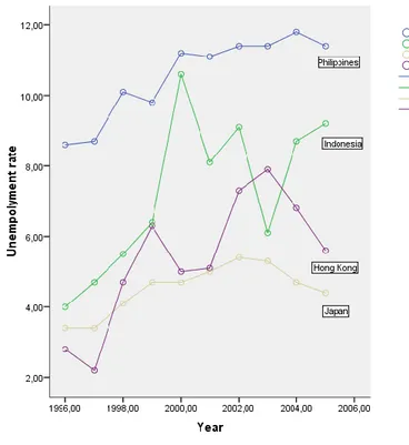
In order to see how the financial crisis affected each respective country a measure that can be observed is the rate of unemployment of each country before and after the crisis hit. Be-low there are two figures (5.1.2 and 5.1.2) representing the level of unemployment in each country from the years shortly prior to the crash until year 2005 after the crisis hit.

Figure 5.1.1

Unemployment after 1995

Prior to the break-out of the crisis in 1997 the unemployment rates in the region had been varying both up and down. The boom in the East-Asian economies generated a lot of job opportunities and the unemployment numbers started to decrease in certain countries. The countries that had seen an overall decrease in their unemployment prior to the crisis are Thailand, South Korea, Malaysia, and the Philippines. Whilst the unemployment seems to be increasing in Indonesia and Japan, the figures for Singapore and Hong Kong are fluc-tuating up and down.

After the crisis the numbers changed drastically for each country, with the change in 1997 to 1998 ranging from a rather small change percentage points in Singapore of 0.8 up to 4.2 percentage points change in South Korea. Observing Indonesia‟s unemployment we can

see that it has been drastically increasing after the crisis. Japan and Singapore were not dras-tically affected due to them not being directly hit by the crisis, but the contagion effect caused them to experience an increase in their numbers for 1997 to 1998. The plotted path for Japan is rather horizontal after 1998 indicating almost no change whilst Singapore`s plotted line fluctuates up and down.

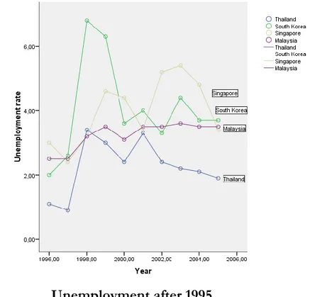
Figure 5.1.2

Unemployment after 1995

From observing the figures it is quite apparent that the financial crisis had an effect on the unemployment rates of each respective country. These countries were all affected in differ-ent magnitudes and the developmdiffer-ent of their figures has taken differdiffer-ent paths. Thailand and South Korea have started decreasing their unemployment rates as is seen in the figures above, attempting to move back to the levels prior to the crisis. The unemployment rates of the other countries have either increased or stagnated around the level just after the cri-sis. But it is clear that none of the countries have come back to the level of unemployment prior to the crisis and therefore have not recovered in this aspect.

5.2 Gross Domestic Product

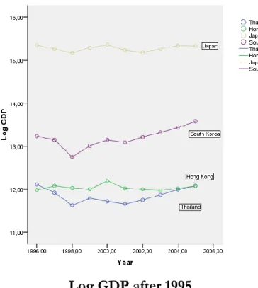
Japan, which is the most closed economy among those presented, was the first to recover to its initial Gross Domestic Product (GDP) level, already within the second year of the crisis (1999). The figures 5.2.1 and 5.2.2 below, illustrate the level of the log of GDP for each respective country in relation to time. From the figures one can also see the difference in the size of all these economies, and observing the non logged GDP levels in appendix 7, Japan is more than eight times as large as South Korea in terms of GDP in 1998, which is the second largest economy in the sample set. South Korea recovered in 2002 to the same GDP level as 1997 and they have continued to grow after this at a decreasing growth rate

Figure 5.2.1

Log GDP after 1995

Hong Kong was another country that recoverd fast; they were back to their initial GDP in the year 2000 which deviates from their other figures. After this their growth slowed down and had a decreasing trend with the GDP just below the 1997 level for the years 2001 to 2004. They were the only country that recovered only to fall back down below their 1997 level as illustrated by figure 5.2.1.

Thailand and Philippines were the countries that took the longest to recover; they returned to their 1997 level in 2004. The fact that Thailand was amongst those who took the longest to recover is quite understandable since this is where the Asian financial crisis broke out. Singapore‟s GDP, as illustrated below in figure 5.2.2, also experienced a very low level of growth in GDP after the crisis, but it has been generally rising. Observing the GDP in rela-tion to recovery in the figure, it shows that the GDP almost returned to the 1997 level much earlier than in 2004, but the numbers were just below this level. At the same time Singapore is the most open economy in the sample set and was among the three countries that took the longest to recover.

Both Indonesia and Malaysia recovered within six years (2003) and they have continued to grow after this. The figures in 5.2.2 illustrate a rather steep increase in the growth of the GDP for each of these respective countries.

Figure 5.2.2

Log GDP after 1995

In terms of the GDP all the countries recovered by 2004. The different growth rates and the need to recover is dependant on how each country was affected after 1997, which is discussed in the next section.

5.3 Current Account

The current account balance, as mentioned earlier, is altered mainly by the exchange rate and the amount of disposable income there is within a country. To determine the effect that a change in relative prices of national outcome will have on the current account we need to consider the import and export sector of the country. If foreign products become more expensive than domestic products due to an increase in the real exchange rate, all else equal, a foreign output now buys more domestic outputs, the foreign consumption pattern will move in favour of domestic export. This change will improve the current account of the domestic country. As one considers the same real exchange rate increase effect on im-port one will see a more complicated situation. To respond to the price shift the domestic consumer will decrease their unit consumption of the more expensive foreign goods. Im-port is measured in terms of domestic outputs, so increases in real exchange rates does not imply that import have to fall. “Because a rise in the real exchange rates tends to raise the value of each units of imports in terms of domestic output units, imports measured in do-mestic output units may rise as a result of a rise in the real exchange rate even if imports decline when measured in foreign output units” (pg.410). Because of this import can rise or fall as a consequence of a real exchange rate increase, this creates an ambiguous effect of on the current account. The „volume effect’ is when consumer‟s spending effects import and export quantities, whilst the “value effect changes the domestic output worth of a given vol-ume of foreign imports” (pg. 410). Krugman & Obstfeld assvol-ume that the volvol-ume effect

the import and export order of goods and services are usually planned a certain time ahead. Thus when a depreciation of the currency occurs, the previously ordered goods may reflect the consumption decisions made under the old exchange rate. It takes time for the new or-ders to adjust to the new price schemes and it takes time for the consumers to adjust. This time lag also has a certain effect on the pass-through of the exchange rate to the import prices, in turn affecting the trade volumes within a country. The time lag that this deprecia-tion causes, and the theory behind, it is referred to as the J-curve (Krugman & Obstfeld, 2006).

The disposable income affects the current account a bit differently. An increase in the dis-posable income will cause the current account to decrease, because domestic consumption goes towards all goods including imports, whilst the opposite effect is apparent for a de-crease in the disposable income (Krugman & Obstfeld, 2006).

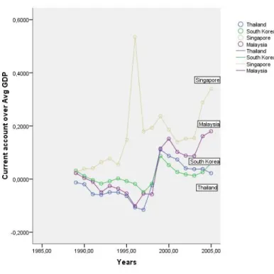
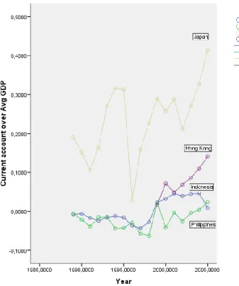
Observing figures 5.3.1 and 5.3.2 for each of the country‟s current accounts one can see that all of the countries that were directly hit by the crisis experienced negative current ac-counts. With the outbreak of the crisis these countries current accounts went from negative to positive within a period of one year. The magnitude of the reversal varied in size from country to country and in turn affected each country‟s GDP. According to current account reversal theory put forward by Edwards (2004) the magnitude of the reversals effect on GDP is dependent on the degree of trade openness of each respective country.

The observations in these figures were calculated by the following formula:

Where CAt is the current account of a country in year t and Avg GDP is the GDP average

for that country for the years 1998 to 2005. The formula illustrates the form of the figures below, how each current account changed over a normalised GDP.

Observing the figures for the current accounts of each respective country all the countries that were directly hit by the crisis experienced a current account reversal, with the excep-tion of Hong Kong. The figures for Hong Kong prior to 1998 are missing and a possible explanation to this is the change of government in 1997.

Figure 5.3.1

Current account over average GDP

The most closed economy, Japan, along with the most open economy, Singapore, both have positive figures from 1989 to 2005 in terms of their current account. Comparing these to the other countries all of them have negative current account figures prior to 1998 with the exception of South Korea who had positive figure in 1989 and 1990.

After 1997 the majority of the countries current account figures are positive and show gen-erally higher values than those before 1998. The Philippines experienced negative current account figures between 1999 to 2002.

Figure 5.3.2

Current account over average GDP

The magnitude of the reversal of all these country‟s is shown in the table 5.3.1 below: Table. 5.3.1

Current Account Reversal

Country Reversal 1997 % Japan No reversal Indonesia 4.29 Korea 11.7 Philippines No reversal 2.37 Thailand 12.6 Malaysia 13.2

Hong Kong Data not available

Singapore No reversal

As mentioned above the data prior to 1997 was missing for Hong Kong and thus we could not calculate or conclude if there had been a reversal in Hong Kong‟s current account. The Philippines is another exception to the theory; they experience a change in their current ac-count from negative to positive, but this change was only 2.37% of GDP, whilst a reversal is defined as at least a 4% of GDP.

Thus according to the theory of Edwards along with our hypothesis the results of countries that were affected by current account reversals and the effect on their GDP is correct with the acceptance of Malaysia.

5.4 The relation of the 1998 GDP drop to Openness

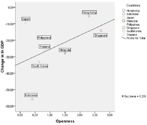
The theory of current account reversal says that the more closed an economy is the larger the negative effect of on GDP, whilst the more open the smaller is the effect. Figures 5.4.1 and 5.4.2 below illustrate this relationship. The countries that experienced a current ac-count reversal were mentioned in the previous sector. The figures in this section show the relation and effect of a reversal on the GDP.

Edwards claimed that the effect of a current account reversal will always have a negative ef-fect on the level of GDP in a country but the size of this is dependent on the trade open-ness. The more open a country is the smaller is the negative effect of the reversal on the GDP, whilst a relatively more closed economy GDP will suffer more.

Japan is one of the largest economies in the world and the difference in the level of their GDP in relation to the other countries in this sample is very substantial. In order to give a more true representation they are removed from the figure below 5.4.2.

The figures below, 5.4.1 and 5.4.2, illustrate the theory put forward by Edwards (2004), that the more closed an economy is the more affected it is by a current account reversal. The figures show that on average as the countries are increasing in openness the less they are af-fected by the crisis in terms of the magnitude of the drop of their GDP from the crisis. The trend line illustrates that increasing openness decreases the magnitude of the drop in GDP.

Among the countries presented in figure 5.4.1 Indonesia is the most closed economy at the time of the crisis with 0.44 degrees of openness, thus in accordance with the reasoning they should also be the most affected after the crisis. Analysing the change in GDP from 1997 to 1998 there is a drop calculated to be 55.76%; the level of GDP more than halved in one year. The drop is quite substantial and a drop of this magnitude causes major shocks in the economy and the establishment and thus in there is great potential for growth in the short run in order to return to the same level of GDP as before.

South Korea is in turn the second most closed economy amongst the affected countries. They show a drop of 33.09% in their GDP from 1997 to 1998, their GDP almost halved in the year of the crisis making them the second most affected by the crisis. Like all other countries they have the potential to recover fast and it is the third fastest growing country after the crisis. Thus both Indonesia and South Korea are in line with the theory that the more closed the economy is the more affected, the exception to this is Malaysia. They are the third most affected country but at the same time the third most open after Singapore, who was not affected in the same magnitude as Hong Kong. The drop in GDP for Malay-sia from 1997‟s level to 1998 was 27.95% of GDP.

Figure 5.4.1

The change in log GDP in 1998 in relation to Openness

Figure 5.4.2

The change in log GDP in 1998 in relation to Openness

without Japan

Hong Kong is the second most open economy in the analysis and as according to the the-ory of openness they are the least affected country in terms of GDP. The difference from 1997 to 1998 is only a slight drop of 5.33%. Hong Kong was not deeply affected in a large drop in their GDP but on the other hand their growth took a substantial hit.

Thailand is either the fourth most open country or the fifth most closed country depending on how you see it. They are on the other hand the fourth most affected, switching places with the Philippines who are fifth, but should be fourth according to the theory. This can though be explained by the fact that the degree of openness between these countries is very similar, Thailand with 0.8 degrees of openness and the Philippines with 0.77. Comparing the drops from 1997 to 1998 in GDP for each respective country Thailand was more af-fected with a drop of 25.91% whilst the Philippines had 20.85%. One logical explanation apart from the openness not being very different is that Thailand was the actual origin of the crisis and thus they should be and were more hit by speculative attacks as other coun-tries were affected, in comparison to the Philippines. (See appendix 8)

Japan and Singapore are special cases since they did not experience a reversal and were not directly hit by the crisis. Even though these countries were not affected in terms of a rever-sal they were both negatively affected by the contagion effect causing a negative climate in the Asian economic area. Contagion as discussed in the previous research sector explains the spreading of the crisis to so many countries and also why it occurred so fast. The main reasons for the contagion effect is based on that the affected countries are all based on similar macroeconomic policies and at the same time are very well integrated through trade. Thus in accordance with this, when an external shock causes problems in one economy it will pass through very easily to the others.

In this case Singapore experienced the largest fall of the two with a decrease of 14.05% in their GDP whilst Japan only had a decrease of 9.44%. The drop in these countries‟ GDP plays a certain role but for Japan the need to recover to their initial growth rate is not as large as Singapore‟s. This is because Japan is one of the largest economies in the world and can handle this sort of debt and recover in due time, whilst Singapore is a very small econ-omy which relies highly on their imports and exports as a contribution to GDP.

To test the validity of these results, the estimation results for the trend lines in Figure 5.4.1 and 5.4.2 (regression (1)) are presented in Table 5.4.1 below.

Table 5.4.1

Regression of change in log GDP on openness

All countries All countries except Japan

Slope coefficient 8.455 13.013 t-statistic p-value 1.358 0.223 2.722 0.042 0.225 0.597

of 1 %. As we can see from figure 5.4.1, and as confirmed by the sign of the estimated slope coefficient in table 5.4.1 when all countries are used, there is an increase in log of GDP a decreasing negativeness in that change as the openness of a countries is increasing. This is not in line with the stated hypothesis that the more open an economy is the more vulnerable they are to an external shock. As Japan is removed from the regression the same conclusion is reached. In figure 5.4.2 one can see a steeper trend line than in figure 5.4.1, which is also reflected in the regression results, strengthening the conclusion that, in other words, the more closed an economy is the more affected it would be.

5.5 Openness of countries and growth

This section analyses what relation the openness of a country has on its average growth level after the crisis.

The figure 5.5.1. below shows a decreasing trend between GDP growth and increasing openness. The most closed economy in the sample, Japan, was the third largest economy in the world in 2005 (CIA World factbook, 2005) measured in purchasing power parity of GDP and therefore it is not surprising that they are more closed than the other countries. The growth level is very low but they are not in the same need to grow as other countries as explained by the theory of openness, that a large economy can afford to be more closed. At the same time the growth rate has not changed much from the years prior to the crisis; it has been rather maintained. Furthermore the case of Hong Kong is also very special since it has been experiencing an average decrease in its growth rate level after the crisis. In order to give a more true representation of how the countries growth rates were affected after the crisis, another figure was provided excluding Japan and Hong Kong.

Figure 5.5.1

The effect of openness on average growth after 1997

Figure 5.5.2

The effect of openness on average growth after 1997 -

With-out Hong Kong and Japan

Source: IMF financial statistics yearbook

Figure 5.5.2 illustrates how the openness of each country is related to the rate of growth af-ter 1997, measured by the gradient of the growth trend line (see appendix 9). The figures for openness are taken from appendix 5. Observing the figure we can see that all countries are following the same pattern, that the more open an economy is the smaller the growth is after the crisis.

The countries that are most affected when a crisis occurs are usually the most eager and in need to recover faster than the less affected naturally. Since they were hit in a larger magni-tude they have a larger amount to recover until they return to the level before the crisis. The theory says that the more open a country is the more vulnerable they are to an external shock, at the same time they are more able to handle a shock with the help of their trade balance. Thus if a more closed economy is hit they do not have the same abilities to deal with the crisis and should thus be more affected by a crisis.

As Thailand was the origin of the crisis and Indonesia, Malaysia and South Korea were the most affected and were considered in trouble, the International Monetary Fund offered to help all of these countries in their financial situation along with other organisations such as the World Bank. All these except Malaysia accepted to be helped both financially and with policies. South Korea, the largest of the economies, received the most funding - a total of 58.4 billion dollars US, with 21.1 billion dollars US coming from the IMF. Indonesia which is second largest in terms of GDP received 49.7 billion dollars US whilst Thailand received 17.2 billion dollars US (IMF, 2005).

With funding from the IMF and the World Bank these countries have had a helping hand in their struggle to recover from the crisis. Indonesia, which was the most affected country, was also in need to recover the fastest. Looking at their growth rate after the crisis they are the second fastest growing after the crisis. Figure 5.5.1 shows that Malaysia has the highest

should have the fastest growth rate to recover faster. Thus Indonesia and South Korea are in line with the logic but Malaysia is going against the logic slightly.

Both the Philippines and Thailand have very similar levels of growth after the crisis, similar to how they were affected by the crisis. In this case the Philippines has been growing slightly faster than Thailand, even though Thailand was in larger need to grow faster in ac-cordance to what magnitude they were affected in. The reason again for Thailand not be-ing able to maintain a higher growth is due to it bebe-ing the origin of the crisis and a lot of structural reforms taking place in the country.

The observation for Hong Kong which was excluded in figure 5.5.1 since it is the only country with a negative average growth from 1997 to 2005. In other words the crisis has af-fected Hong Kong very negatively but in a different sense in comparison to the other countries. (See appendix 7)

Statistics for the trend lines are presented in Figures 5.5.1 and 5.5.2 (regression (2)) above are presented in table 5.5.1 below.

Table 5.5.1

Regression of average Growth after 1997 on Openness

All countries after 1997 All countries after 1997 except Japan and Hong Kong

Slope Coefficient -0.103 -0.020 t-statistic p-value -0.729 0.494 -0.745 0.498 0.081 0.122

Whether one decides to have all the countries in the regression or exclude Japan and Hong Kong, the outcome is similar. As is seen from figure 5.5.1 and 5.5.2 and as confirmed by the sign of the estimated slope coefficients in table 5.5.1 there is a negative relation, show-ing that the GDP growth will decrease as average openness is increasshow-ing. However for both of the regressions one can not reject the null hypothesis that there is no linear effect of openness on average growth. At the same time the R-squared values for the regressions in table 5.5.1 are both very low, meaning that the goodness of fit of the regressions is not to strong. In other words both the figures and regressions show that the relation between openness and growth is not so strong.

As mentioned earlier the IMF along with the World Bank provided a lot of funding to-wards South Korea and Indonesia who were the second and third most growing economies after the crisis. At the same time they are the two most closed countries that were affected, and the two most affected in terms of the magnitude of the drop in GDP. The countries that were most affected are in greater need to recover fast than those less affected. This could have certain implications for testing the theory put forward.

An interesting observation is that for all the countries the average openness increases in the period 1998 to 2005 in comparison to the period before the crisis 1989 to 1996 even though these countries were experiencing a very large growth period at that time (see

ap-pendix 5). An explanation for this is that the countries had to open their trade sector in or-der to recover from the drop that they experienced after the crisis. If a country trades more this takes a larger percent of their total GDP, thus they become more open.

6

Conclusion

The Asian financial crisis effectively put an end to what was known as the „Asian miracle‟. As the thesis shows, many countries in Asia were affected, all of them in different magni-tudes. The thesis shows what a financial crisis can do to a region and the economic climate. What is important to remember is that there are many implications on the rest of the world when a crisis of this magnitude hits a large economic region as Asia. This is something that has not been covered within the thesis due to the magnitude of information and knowledge one would have to have in order to draw any relevant conclusion.

This thesis shows that the degree of openness has an effect on how a country is affected during a financial crisis in terms of its current account, which in turn affects the growth of its GDP. The first regression results show that the effect of openness on the drop in GDP after the asian financial crises, that the more closed an economy is the larger the drop in GDP after a crisis. Looking further at how openness affects growth in the years after the crisis there is no direct indication of a linkage of that the more open the higher the growth rate will be. The descriptive statistics and the regression show that the more closed a coun-try is the more they will grow (although this is not statistically significant) which was not in accordance to the hypothesis.

One conclusion that can be drawn from the analysis is that all the countries have recovered in terms of their level of GDP. But a total recovery has not been achieved since the unem-ployment rate prior to the crisis is lower in all countries than what it is for all the years af-ter. It is important though to remember that the growth levels for the majority of the coun-tries was very high prior to the crisis, something which they all had not experience before and thus it is hard to expect for these countries to return to the same level under eight years.

Suggestions for further research that could be of use and give a more concentrated direct answer is to analyse more deeply a very specific area such as only looking at the current ac-count effect. Since there is a problem to explain a valid result when one takes into many aspects into their analysis.

Furthermore a suggestion is to analyse the affected trading partners who are located in an-other region to see if they were affected in the same way as the countries in the Asian re-gion.

References

Alesina, A. & Wacziarg, R. (1997) Openness, country size and government. Journal of Public

Economics, 69, 305-321.

Calvo, A. G., Izquierdo, A., Mejia, L. (2003) On the empirics of suuden stops: The relev-ance of Balrelev-ance-sheet effects. Working paper, Interamerican Development Bank

CIA (2005) CIA- World Fact Book 2005. Retrieved on 2008-11-29:

http://www.umsl.edu/services/govdocs/wofact2005/geos/ja.html#Econ

Claessens, S. & Forbes, K. (2001) International Financial Contagion. Dordrecht: Kluwer Aca-demic Publishers

Corsetti, G. Pesenti, P. & Roubini, N. (1999) What caused the Asian currency and financial crisis? Japan and the World Economy, 11, 305-373.

Edwards, S. (2004) Financial openness, sudden stops and current account reversals. The

American economic review. 94(2), 59-64. Papers and Proceedings of the One Hundred Sixtheenth An-nual Metting of the American Economic Association

Edwards, S. (1998) Openness, productivity and growth: what do we really know? The

Eco-nomic Journal, 108, 383-398.

Glick, R. & Rose, A. (1999) Contagion and trade, Why are currency crises regional? Journal

of international Money and Finance, 18, 603-617.

Gujarati, N.D (2003) Basic econometrics. 4th _{edition. Boston: McGraw Hill}

International Monetary Fund (2000) International financial statistics yearbook.Vol. LIII 2000 Washington D.C.: Prepared by IMF statistic Department. Director: Carol S. Carson

International Monetary Fund (2005) International financial statistics yearbook.Vol. LVIII 2005 Washington D.C.: Prepared by IMF statistic Department. Director: Robert W. Edwards International Monetary Fund Staff (2005) Recovery from the Asian Crisis and the Role of the IMF. Retrieved on 2008-12-04:

http://www.imf.org/external/np/exr/ib/2000/062300.htm

International Monetary Fund (2007) International financial statistics yearbook.Vol. LX 2007 Washington D.C.: Prepared by IMF statistic Department. Director: Robert W. Edwards International Monetary Fund (2006) International financial statistics yearbook.Vol. LIX 2006 Washington D.C.: Prepared by IMF statistic Department. Director: Robert W. Edwards Kaminsky, Graciela Laura (2008) Currency crises. The New Palgrave Dictionary of Econom-ics. Second Edition.Eds. Durlauf & Blume.Palgrave Macmillan. Retrieved on 2008-11-04: http://www.dictionaryofeconomics.com/article?id=pde2008_C000468

Law & Smullen.(2008) Financial crisis. A Dictionary of Finance and Banking. Oxford Uni-versity Press, 2008. Oxford Reference Online. Oxford UniUni-versity Press. Retrieved on 2008-10-30:

http://www.oxfordreference.com/views/ENTRY.html?subview=Main&entry=t20.e4506 Montes, M.F. (1998) The currency crisis in Southeast Asia. Singapore: Institute of Southeast Asia Studies

Milesi-Ferretti. G.M. & Razin, A. (1996) Current-account sustainability. Princeton studies in

in-ternational finance, 81.

Milesi-Ferretti. G.M. & Razin, A. (1997) Sharp Reduction in Current Account Deficits: An

Empir-ical Analysis. IMF working paper

Park & Song (2000) Institutional Investors, Trade Linkage, Macroeconomic Similarities, and Contagion of the Thai Crises. Journal of the Japanese and International Economics, 15,

199-224.

Yanikkaya, H. (2003) Trade openness and economic growth: a cross-country empirical in-vestigation. Journal of Development Economics, 72, 57-89.

Data sources:

United Nations UN Comtrade database Retrieved: 2008-10-30 from: http://comtrade.un.org/db/dqBasicQuery.aspx

World Bank Group DDP Quick query database Retrieved: 2008-10-30 from:

http://ddpext.worldbank.org/ext/DDPQQ/member.do?method=getMembers&userid=1 &queryId=135

Appendix 1

Unemployment rates (%) Period Average

Source: International Monetary Fund financial statistics yearbook

Years Thailand South Korea Singapore Malaysia Indonesia Philippines Japan Hong Kong

1989 1.4 2.6 2.2 6.3 2.8 8.4 2.3 1.1 1990 2.2 2.4 1.7 5.1 2.5 8.11 2.1 1.3 1991 2.7 2.3 1.9 4.3 2.6 9 2.1 1.8 1992 1.4 2.4 2.7 3.7 2.7 9.8 2.2 2 1993 1.5 2.8 2.7 3 2.8 9.3 2.5 2 1994 1.3 2.4 2.6 2.9 4.4 9.5 2.9 1.9 1995 1.1 2 2.7 2.8 9.5 3.2 3.2 1996 1.1 2 3 2.5 4 8.6 3.4 2.8 1997 0.9 2.6 2.4 2.5 4.7 8.7 3.4 2.2 1998 3.4 6.8 3.2 3.2 5.5 10.1 4.1 4.7 1999 3 6.3 4.6 3.5 6.4 9.8 4.7 6.3 2000 2.4 4.4 4.4 3.1 6.1 11.2 4.7 5 2001 3.3 4 3.4 3.5 8.1 11.1 5 5.1 2002 2.4 3.3 5.2 3.5 9.1 11.4 5.4 7.3 2003 2.2 3.6 5.4 3.6 10.6 11.4 5.3 7.9 2004 2.1 3.7 4.8 3.5 8.7 11.8 4.7 6.8 2005 1.9 3.7 3.4 3.5 9.2 11.4 4.4 5.6

Appendix 2

Unemploymen

Source: International Monetary Fund financial statistics yearbook Years Thailand

South

Korea Singapore Malaysia Indonesia Philippines Japan

Hong Kong 1988 929000 435000 46000 482000 2106000 1954000 1550000 38000 1989 433000 463000 31000 389000 2083000 2009000 1420000 30000 1990 710000 454000 26000 315000 1952000 1993000 1340000 37000 1991 869000 436000 30000 314000 2032000 2267000 1360000 50000 1992 456000 465000 43000 271000 2199000 2263000 1420000 55000 1993 646000 550000 44000 317000 2246000 2379000 1656000 57000 1994 423000 489000 44000 228000 3738000 2622000 1920000 56000 1995 375000 419000 47000 248000 2704000 2098000 96000 1996 354000 425000 54000 217000 4287000 2546000 2250000 87000 1997 293000 557000 46000 215000 4197000 2640000 2303000 71000 1998 1138000 1463000 62000 287000 5062000 3043000 2787000 154000 1999 986000 1353000 90000 314000 6030000 3017000 3171000 208000 2000 813000 974000 96000 299000 5813000 3459000 3198000 167000 2001 119000 899000 72000 342000 8005000 3653000 3395000 175000 2002 826000 752000 110000 344000 9132000 3874000 3588000 256000 2003 761000 818000 111000 370000 3936000 3504000 277000 2004 741000 868000 367000 4249000 3134000 241000 2005 666000 887000 372000 4145000 2940000 201000

Appendix 3

PA = Population growth (annual %) PT = Population Total

Country

Name Series YR1989 YR1990 YR1991 YR1992 YR1993 YR1994

Hong Kong PA 1,0359 0,3213 0,8292 0,8397 1,7178 2,2520 Hong Kong PT 5686200 5704500 5752000 5800500 5901000 6035400 Indonesia PA 1,7688 1,7938 1,7179 1,6420 1,5662 1,4903 Indonesia PT 175063344,00 178232000,00 181320358,03 184322300,55 187231804,74 190042962,43 Korea, Rep. PA 0,9602 1,1472 0,9264 0,9088 0,8960 0,8971 Korea, Rep. PT 42380000 42869000 43268000 43663000 44056000 44453000 Malaysia PA 2,8857 2,7980 2,6923 2,6007 2,5408 2,5242 Malaysia PT 17603827 18103341 18597361 19087376 19578569 20079056 Japan PA 0,4094 0,3414 0,3104 0,2482 0,2468 0,3407 Japan PT 123116000 123537000 123921000 124229000 124536000 124961000 Philippines PA 2,3839 2,3567 2,3309 2,3069 2,2767 2,2396 Philippines PT 59799928 61225972 62669859 64132377 65609257 67095197 Singapore PA 2,9429 3,8814 2,8504 3,0038 2,5306 3,1343 Singapore PT 2931000 3047000 3135100 3230700 3313500 3419000 Thailand PA 1,2696 1,2355 1,2021 1,1701 1,1472 1,1347 Thailand PT 53624669 54291323 54947895 55594639 56236105 56877831 Country

Name Series YR1995 YR1996 YR1997 YR1998 YR1999 YR2000

Hong Kong PA 1,9801 4,4386 0,8325 0,8348 0,9551 0,8816 Hong Kong PT 6156100 6435500 6489300 6543700 6606500 6665000 Indonesia PA 1,4144 1,3947 1,3750 1,3554 1,3357 1,3160 Indonesia PT 192750000,00 195457134,30 198163293,95 200867393,24 203568332,74 206265000,00 Korea, Rep. PA 1,4295 0,9535 0,9379 0,7220 0,7104 0,8355 Korea, Rep. PT 45093000 45525000 45954000 46287000 46617000 47008111 Malaysia PA 2,5320 2,5463 2,5377 2,4900 2,3930 2,2654 Malaysia PT 20593952 21125065 21668014 22214316 22752310 23273615 Japan PA 0,3818 0,2564 0,2621 0,2527 0,1897 0,1736 Japan PT 125439000 125761000 126091000 126410000 126650000 126870000 Philippines PA 2,1991 2,1547 2,1153 2,0913 2,0871 2,0946 Philippines PT 68587012 70080887 71579068 73091778 74633277 76213060 Singapore PA 3,0390 4,0644 3,3566 3,3979 0,7989 1,7329 Singapore PT 3524500 3670700 3796000 3927200 3958700 4027900 Thailand PA 1,1275 1,1270 1,1203 1,0907 1,0307 0,9509 Thailand PT 57522738 58174703 58830127 59475310 60091464 60665589

http://ddp-ext.worldbank.org/ext/DDPQQ/report.do?method=showRepo

Country Name Series YR2001 YR2002 YR2003 YR2004 YR2005

Hong Kong PA 0,7325 0,3667 0,3667 0,3667 0,3667 Hong Kong PT 6714000 6738663.76 6763418.13 6788263.43 6813200 Indonesia PA 1,3240 1,3320 1,3400 1,3480 1,3560 Indonesia PT 209014094,83 211816758,36 214674159,94 217587497,82 220558000,00 Korea, Rep. PA 0,7321 0,5509 0,4904 0,4856 0,4399 Korea, Rep. PT 47353519 47615132 47849227 48082163 48294143 Malaysia PA 2,1308 2,0130 1,9186 1,8560 1,8156 Malaysia PT 23774848 24258296 24728210 25191441 25652985 Japan PA 0,2197 0,2325 0,2140 0,0337 0,0094 Japan PT 127149000 127445000 127718000 127761000 127773000 Philippines PA 2,1043 2,1055 2,0944 2,0674 2,0286 Philippines PT 77833803 79489929 81172343 82867926 84566163 Singapore PA 2,6967 0,9141 -1,4764 1,2534 2,3505 Singapore PT 4138000 4176000 4114800 4166700 4265800 Thailand PA 0,8633 0,7862 0.730080774166714 0,7034 0,6974 Thailand PT 61191592 61674588 62126510 62565066 63002911

Appendix 4

Current account in millions of US$

Years Thailand

South

Korea Singapore Malaysia Indonesia Philippines Japan

Hong Kong 1988 -1654 14505 1937 1867 -1397 -390 79250 1989 -2498 5361 2964 315 -1108 -1456 63210 1990 -7281 -2003 3122 -870 -2988 -2695 44080 1991 -7571 -8137 4880 -4183 -4260 -1034 68200 1992 -6303 -3944 5915 -2167 -2780 -1000 112570 1993 -6364 990 4211 -2991 -2106 -3016 131640 1994 -8085 -3867 11400 -4520 -2792 -2950 130260 1995 -13554 -8507 41373 -8469 -6431 -1980 11040 1996 -14691 -23006 13854 -4596 -7663 -3953 65880 1997 -3024 -8167 14919 -4792 -4889 -4351 94350 1998 14048 40558 18286 9529 4096 1546 120700 2507 1999 11050 24522 14361 12604 5783 -2874 106870 10248 2000 9313 12251 10728 8488 7992 -225 119660 6993 2001 5101 8033 11760 7287 6901 -1744 87800 9786 2002 4691 5934 11918 7190 7824 -279 112450 12412 2003 4772 11950 22317 13381 8107 288 136220 16470 2004 2759 28174 26318 14871 1563 1633 172060 15728 2005 -7857 14981 33212 19980 2338 165780 20233

Appendix 5

Openness to Trade

Year Thailand Korea South Singapore Malaysia Indonesia Philippines Japan Hong Kong 1989 0.6322 0.5363 3.1280 1.2005 0.3758 0.4460 0.1641 2.1133 1990 0.6585 0.5096 3.0742 1.3012 0.4142 0.4790 0.1716 2.1415 1991 0.6701 0.4962 2.8922 1.4155 0.4281 0.4774 0.1589 2.2383 1992 0.9011 0.4783 2.7243 1.3498 0.4392 0.4767 0.1514 2.3359 1993 0.6648 0.4566 2.7320 1.3681 0.4112 0.5515 0.1386 2.2834 1994 0.9566 0.4654 2.8163 1.5627 0.4064 0.5619 0.1402 2.3108 1995 0.7545 0.4931 2.8738 1.6762 0.4254 0.6171 0.1478 2.5411 1996 0.7016 0.4826 2.7616 1.5304 0.4075 0.6638 0.1635 2.3859 1997 0.7942 0.5193 2.6712 1.5524 0.4399 0.7715 0.1780 2.2550 1998 0.8513 0.6192 2.5475 1.8077 0.7932 0.9328 0.1730 2.1478 1999 0.8161 0.5773 2.7228 1.8757 0.5165 0.8851 0.1662 2.2745 2000 1.0601 0.6429 2.9290 1.9765 0.5772 0.9865 0.1837 2.1140 2001 1.0907 0.5994 2.7649 1.8194 0.5413 0.9407 0.1835 2.3469 2002 1.0382 0.5702 2.7266 1.8062 0.4505 0.9912 0.1921 2.4892 2003 1.0867 0.6047 3.1649 1.7904 0.3975 0.9868 0.2018 2.8731 2004 1.1735 0.6933 3.3966 1.8473 0.4173 0.9848 0.2212 3.1961 2005 1.2939 0.6895 3.5729 1.8547 0.4996 0.9176 0.2436 3.3317 AVG 89-96 0.7424 0.4898 2.8753 1.4255 0.4135 0.5342 0.1545 2.2938 AVG98-05 1.0513 0.6245 2.9782 1.8472 0.5242 0.9532 0.1956 2.5967 Avg 89-05 0.8908 0.5549 2.9117 1.6315 0.4671 0.7453 0.1753 2.4340

Source: Import & Export figures from Comtrade Database and GDP from DDP World Bank Quick Query Database

Appendix 6

GDP Growth rate (%)

Years Thailand Korea South Singapore Malaysia Indonesia Philippines Japan Hong Kong

1988 13 11 11 10 6 7 7 8 1989 12 7 10 9 9 6 5 8 1990 11 9 9 9 9 3 5 4 1991 9 9 7 10 9 -1 3 6 1992 8 6 6 9 7 0 1 6 1993 8 6 12 10 7 2 0 6 1994 9 9 12 9 8 4 1 6 1995 9 9 8 10 8 5 2 2 1996 6 7 8 10 8 6 3 4 1997 -1 5 8 7 5 5 2 5 1998 -11 -7 -1 -7 -13 -1 -2 -6 1999 4 9 7 6 1 3 0 3 2000 5 8 9 9 5 6 3 8 2001 2 4 -2 0 4 2 0 0 2002 5 7 4 4 4 4 0 2 2003 7 3 3 6 5 5 1 3 2004 6 5 9 7 5 6 3 8 2005 5 4 7 5 6 5 2 7