VIIsartryck _
110 A 1986
A comparison of two methods for estimating
the effect of a countermeasure in the pre-sence of regression effects
Stig Danielsson
Reprint from Accident Analysis & Prevention, vol. 18
Väg06/1 Efi/( Statens väg- och trafikinstitut (VTI) * 581 01 Linköping IIIStlt"tet Swedish Road and Traffic Research Institute * S$-581 01 Linkoping Sweden A
Printed in Great Britain. © 1986 Pergamon Press Ltd.
A COMPARISON OF TWO METHODS FOR ESTIMATING
THE EFFECT OF A COUNTERMEASURE IN THE
PRESENCE OF REGRESSION EFFECTS
STIG DANIELSSONSwedish Road and Traffic Research Institute (VTI), S-581 01 Linköping, Sweden
(Received 2 March 1983; in revised form 16 May 1985)
Abstract The report studies the problem of estimating in a non-experimental before-and-after inves-tigation the effect of a countermeasure on the number of traffic accidents at road junctions. The accidents are assumed to occur according to a Poisson process with different intensities at different junctions. The junctions studied in this investigation are assumed to have been selected with the blackspot-technique, i.e. junctions with high numbers of accidents during the before-period have been chosen for the inves-tigation. In the mathematical model this has the consequence that the number of accidents occurring during the before-period at a selected junction has a truncated Poisson distribution. During the after-period the number of accidents has a Poisson distribution (without restrictions), so that the number of accidents on the average decreases between the periods even if the countermeasure has no effect. The magnitude of this regression effect is studied in the report. The observed numbers of accidents during the before and after period are used to estimate the pure effect of the countermeasure both with an intuitive method and with the maximum likelihood method. The characteristics of the two methods of estimation are illustrated with the aid of simulation studies. In general the maximum likelihood method appears preferable, mainly because it produces estimates with higher precision.
1. INTRODUCTION
One problem occurring in many before-and after studies is the regression effect. This is caused by the selection procedure, which implies that experimental units are drawn with regard to the outcomes of the variable studied during the before-period. Assume, for example, that a study is to be made of the effect on the number of traffic accidents of a certain countermeasure implemented at road junctions. Traditionally these countermeasure-and-effect studies are made by selecting a number of road junctions which have especially high accident levels (i.e. where the number of accidents is considerably above the expected). This means that even if the countermeasure has no effect, the number of accidents at the junctions studied will decrease
after the countermeasure has been implemented, since the number of accidents tends to return
to the average.
The problem with regression effects in different types of before-and-after studies has been known for a long time. However it is only recently that it has been appreciated by researchers in the traffic safety field how large this problem may be. In empirical studies Briide and Larsson [1982] observed regression effects of 25 65% for the number of traffic accidents at rural road junctions. Hauer [1980a, 1980b] has described the problem with regression effects in many ways and has given a method for estimating the effects (see Section 4.1). Hauer et al. [1983] have studied the accuracy of the proposed estimator. Hauer s method is founded on a mathe-matical model specifying the number of accidents to be truncated Poisson distributed in the before-period. This is also the basis in our paper (see Section 2).
In practice, the regression effect is not of primary interest. Instead, we are concentrating our efforts in estimating the pure effect of the countermeasure. This is done in this paper by utilizing Hauer s estimator of the regression effect, but also by using the method of maximum likelihood (see Sections 4 and 5). In Section 6 we provide approximate confidence intervals for the countermeasure-effect. The different estimators and confidence intervals are compared in Section 7 by means of simulation studies. In Section 3 we study the expected regression effect by utilizing the truncated Poisson distribution; the purpose is merely to demonstrate the magnitude of the regression effect.
14 S. DANIELSSON
2. FORMULATION OF THE PROBLEM
For the sake of simplicity we shall formulate the problem by means of an example. Assume that we wish to study the effect of a countermeasure implemented at road junctions. Consider junction no. i and let
X,- = the number of accidents during a period before the countermeasure.
We assume in the model that different X,- are independent and that they have a Poisson distribution with expected value mi, i.e. the probability of obtaining r accidents at the junction is
p,(m,.) = P(X, = r) = e mi l,
r = 0, 1, 2. . . .
(1)
r.
Note that the expected number of accidents m, varies from junction to junction, mainly due to different traffic ows.
For simplicity we assume that the period studied after the countermeasure is implemented is of the same length as the before-period, and that the traffic pattern remains the same. For junction no. i we set
Y,- = the number of accidents after the countermeasure has been implemented.
and can then assume that different Y,- are mutually independent and also independent of all X,.
In addition all Y,- are Poisson distributed. '
We assume that the effect of the countermeasure is proportionally of the same magnitude at all junctions, i.e. we assume that Y, has a Poisson distribution with parameter a - m,. The appropriateness of this assumption may be questionable. Probably the effect of the counter-measure varies with different m,, according to, among other factors, the varying number of other countermeasures which have presumably been implemented at the junctions. Having no knowledge of these factors there is no justification in working with any other model than this simple multiplicative model. The model implies that the probability of obtaining r accidents at the junction after the countermeasure is
0Lm, (am,-f
p,(am,.) = P(Y, = r) = e
r, ,
r = o, 1, 2, . ..
(2)
The countermeasure will have had no effect if or = l, a positive effect if a < 1 and a negative
effect if a > 1.
Using a sample of road junctions we wish to estimate a and assess the uncertainty of the estimate. The estimation problem is simple if the sample is made without regard to the observed numbers of accidents during the before-period. However this is not the case in practice. Instead junctions with especially high numbers of accidents, blackspots, are chosen.
We make the assumption that junction no. i will be included in the selection only if the number of accidents X,- is at least k,. This means that for junction no. i in the sample the number of accidents X,- before the countermeasure is at least k,- and the probability of r accidents is
1 m?
P;(mi) : P(Xi' : r) : ___ .e miF; ' : ki, ki+19 . -- (3)
X,~ is said to have a truncated Poisson distribution.
The number of accidents Y, after the countermeasure is not influenced by the selection
procedure and so the distribution of Y, will still be as stated in (2).
Before we begin estimating oc we shall study in more detail the significance of the truncated Poisson distribution and the regression effect accompanying it.
3. THE TRUNCATED POISSON DISTRIBUTION AND EXPECTED REGRESSION EFFECT
We shall now limit the study to a given junction. LetX have a truncated Poisson distribution so that
p,'(m)=P(X'=r)=M, r=k,k+1...
qk(m) where
pron) = e m % and qk(m) = 2 pron); k z 1.
r=k(4)
Also introduce uk(m) as the expected value of X . The bias B can then be written
3 = ILL/(On)
m,
(5)
i.e. B is the expected difference between the numbers of accidents before and after an ineffective countermeasure. The expected regression effect R is defined according to
B .
lid/((fn) 100. (6)
If we can determine uk(m) it will be easy to study R. Different expressions of the expected value of a truncated Poisson distribution is given in many places in the literature, see for
example Hauer [1980b], Hauer et al. [1982] and Selvin [1974].
_ 00 I = _ : Pk(m)
Mm)
Z rmm)
W) qk-.<m>
m + k_q,.<m>'
(7)
Thus B has the simple expression (cf. Hauer et al. [1983])
B = [(P/(("?) (8)
(him)
while the regression effect will be
R=<1~M>-IOO=M-IOO.
(9)
(Dc Km) CIk 1(m)
It is also interesting to determine the dispersion obtained in the truncated Poisson
distri-bution, which, of course, is less than the dispersion in an unrestricted Poisson distribution. Making use of the results of Hauer et al. [1983] it can be shown that the variance of X ' is
Var[X ] = m (I
km) + WM (1
(m).
(10)
Clk(m) %(m) qk(m)
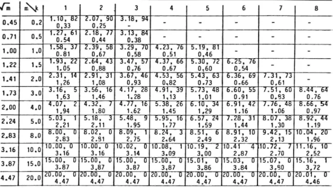
For different m and k it is then easy to compute the parameters derived above, and the results are given in Table 1.
The table shows that the regression effect may be very important. When m is larger than 2k the regression effect is often quite small. When m has the magnitude k a regression effect of 20 40% is obtained. For increased truncations the effect becomes greater and in extreme but nevertheless realistic cases effects of 50 70% may occur.
S. DANIELSSON
16
Table 1. Expected value, standard deviation and expected regression effect in a truncated Poisson distribution
G.
N
1
2 ,
3
4
5
6
7
8
11.10, 82 2.07. 90 3.18, 94 0.45 0.2 0.33 ? 0.25 _ " ' ' " " 1.27, 61 .18, 77 3.13, 84 0.71 0.5 0.54 0.44 0.38 - - - - -1 00 1 0 1.58.737 12.39, 58 3.29, 70 4.23, 76 45.19.481' _ _ _ ' ' 0.81 0,67 0.58 0.51 0,46 1 22 1 5 1.93, 22 2.64, 43 3.47, 57 4,37, 66 45.30, 72 6.25, 76 _ _ ' ' 1.05 0.88 0.76 0.67 0,60 0.54 | 41 2 0 2.31, 14 2.91, 31 43.67, 4 4:53, 56 45.43.463 6.36, 69 7.31, 73 _ ' ' 1,26 1.08 0.93 0.82 0.73 0.66 0.61 | 73 3 0 3.16, 3.56, 16 4.17, 28 4.91.89 5.73, 48 6.60, 55 7.51, 60 8.44, 64 ' ' 1,63 1.46 1.28 1,13 1.01 0.91 0.83 0.76 2 00 4 0 4.07, 2 4.32, 4.77, 16 5.38, 26 46.10, 34 6.91, 42'47Ä76, 48 8 66,754 ' ' 1,94 1.80 1.62 1.45 1,29 1.16 1.06 0.97 2:24 5 0 75,03, 1 5.18, 3 5.48, 9 5.95, 16 6.57, 24 47.28, 31 8.07, 38 8.92, 44 ' 2,21 2.11 1.95 1.77 1.59 1.44 1.30 1.19 2 83 8 O 8.00, 70 8.02, 0 8.09, 1' 8.24, 13 8.51, 6' 8.91, 10 9.42, 15 10 04, 20 ' ' 2.83 2.81 2.75 2.64 2.49 2.32 2.13 1.96 3 16 10 0 10.00, 0 10.00, 0 10.02, 10.08, 1 10.19, 12 10.41 4 10.72, 7 11 16, 10 ' ' 3.16 3.16 3.14 3.09 3.00 .2.87 2.70 2,52 3 87 15 0 15.00,7'0 15.00, 0 15.00, 0 15.00, 0715.01, 40 15.03, 10 15.07, 0 15.16, 11 ' ' 3.87 3,87 3.87 3.87 3.86 3.84 3.80 3,72 4 47 20 0 20.00, 0 20.00, 0 20.00, 0 20.00, 0 .00, 0 20.00, 0 20.00, 0 20.01, 0 ' ' 4.474.47 4.47
4.47 4,47 4.47 4.47 4.46
m = expected value and variance in the non-truncated Poisson distribution k = truncation point
The figures in each matrix element are the expected value, expected regression effect and standard deviation, respectively. The quantities which become uncertain in the calculations due to numerical instability have been excluded from the table. Furthermore they are relatively uninteresting in practice.
We should note that there is a regression effect not only on the expected value but also on the standard deviation. The reduction in the standard deviation is fairly important; it is not unrealistic that Vf; may be halved. This may have serious consequences for statistical methods using predicted number of accidents. Unless adjustment is made for the regression effects, incorrectly small prediction limits will be obtained in addition to an incorrectly high predicted
value.
4. ESTIMATION OF THE EFFECT OF A COUNTERMEASURE AND THE REGRESSION EFFECT FOR A SINGLE SELECTED JUNCTION
We define X and Y in accordance with Sections 2 and 3 and note that the expectation of Y is a - m. A very natural estimator of a is
. Y
a = _. (11)
m
where nä is a suitable estimator of m. The estimator of the regression effect R in (6) is
R
X, _ m 100
X!(12)
and we see that the main problem is to estimate m.
Below we describe three methods of estimating m and a. The first two methods are
motivated on intuitive grounds, while the last method is the method of maximum likelihood.
4.1 Hauer s method
Hauer [1980a] and [1980b] proposes an estimator for the sum of the accidents at n junctions (all truncated at the same k). This result can also be found in an article by Robbins [1977].
The proposal can be interpreted as a desire to estimate
&&
Clk(m)
with a suitable relative frequency. However if only one measurement has been made at the
junction the estimator will be
min)) : {1
ifX' = k
Estimated (611.071) 0 if X' > k i.e. the estimator of m will be (when E[X '] is estimated with X )
. _ 0
ifX = k
'" _ {x'
ifX' > k
(13)
(cf. Hauer et al. [1983]).
As is proven for example by Hauer et al. [1983] the estimator is unbiased with variance
Var[m] = m(1 + B). (14)
This large variance is discussed in detail by Hauer et al. [1983]. 4.2 The moment method
Instead of estimating the conditional probability
Pk(m) Clk(m)
and then implicitly solving m as above, it would be better to try to estimate m directly. An estimator of m with the moment method means that an attempt is made to solve the equation
X = E[X'] = m + B (15)
with regard to m.
The discussion of the solution of eqn (15) is carried out in Section 4.3. 4.3 The method of maximum likelihood
Most often better estimators are obtained with the maximum likelihood method
(ML method) than with the moment method. The ML method implies that the values which
maximizes the likelihood (probability of the observed values) are used as the estimators of the actual parameters. In this case it is therefore possible to estimate both m and a. The likelihood
for the observed values x and y, corresponding to X and Y is [see (3) and (1)].
L(m, a) = p£'(m) 'Py(0tm)-
(16)
Maximizing L is equivalent to maximizing the log-likelihood
w 1r .
l=1nL = (x' + y)1n(m) 1n<27>
am + ylna
ln(x !)
ln(y!). (17)
r==k
Differentiating (17) with respect to m and a and equating to zero gives:
a=y/m
'_ _m._qL__1(_m2 (18)
x .
Qk(m) AAP 18:1 B
18 S. DANIELSSON
The second equation in (18) can be found in Cohen [ 1972] and Selvin [1974] as the ML equation
for estimating m, when observations are made solely on a truncated Poisson distribution.
A straightforward calculation shows that the solutions a* and m* of (18) maximizes the
log-likelihood, and therefore are the ML estimators. It is interesting to note, that a* agrees
with the intuitive & in (11) and that m* is identical to the moment estimator (15).
With a little calculation it can be seen that the function
f(m) = _ CIk 1(m) Clk(m)
is steadily increasing and has the minimal value k at m = 0. Therefore, the ML estimator m* is unique. Furthermore, the function f(m) lies above the line y = m and has an asymptote at y = m. This implies that the estimator m* lies near x for large x' but is always less than x'.
Since the estimator m* is zero for x' = k, it follows that m* S m, where rh is Hauer s estimator in (13). But n : is an unbiased estimator of m, and so the ML estimator m* will on average
underestimate m.
We have seen above that the ML estimator and the moment estimator of m are identical. Comparing Hauer s estimator and the ML estimator, the former at first sight seems better because it is unbiased.
However, our emphasis is to estimate the effect of the countermeasure, and both from a
theoretical and practical point of view, a is not estimable when x = k. But if x > k the estimate of m with Hauer s method is simply x' and so the estimate of or is not corrected at all for the regression effect (this effect is estimated to zero). On the contrary, the ML estimate of m never equals x in this case and the estimate of the regression effect is strictly positive. In this regard the ML estimator of a is better than Hauer s estimator.
Now, the situation discussed in this section is not very practical. In most cases the countermeasure is implemented at several junctions. This is the situation actually treated by
Hauer [l980a, 1980b], and obviously an estimate of or with Hauer s method would be desirable.
5. MAXIMUM LIKELIHOOD ESTIMATION OF THE EFFECT OF A COUNTERMEASURE IMPLEMENTED AT SEVERAL
SELECTED JUNCTIONS
Consider the selected junction no. i, i = 1, 2, . . . , n, and define X,- and Y,- in accordance with Sections 2 and 3. Observe that we assume a common effect of the countermeasure at each
junction.
For the observations
(xi, y1)9(x£9 y2)9 ' ' ' > (xrlza yn)
calculations for the likelihood as in Section 4.3 give
L(a,m1, . . . , m.) ll p;,<m,-)py,.<am.)
l=lnL= aZm, + ice;
+y,-)lnm,-i=l i=1
Zln (Z 310+ Ey,-Ina ln(jl x,- !y,-!>
i=1 r=k, ~ i=1 i=1
,
al
Ey,-8a 2 m,- + T _ O 61 + xi, + Yi _ qk,- l(mi) _ _=_ _D; '=1,2,...,. 19 Öm,- a mi (lic,.(mz) l n ( )Solving (19) gives
E%"
* =
a
2 m,,
(20)
where mi", . . . , m, , are obtained from the equations
Chi (mi) E yi _
xi+Yi=mi' + ? z=l,2,...,n. (21)
51190711 ) Z mi
Obviously we do not now obtain the same type of equations as in (18). The equation system above requires in principle a simultaneous solution with regard to all m,- and will therefore be numerically more troublesome than the corresponding problem in Section 4.3. We can rewrite the equations as
Chi 10710 _ ,
' m _ (xi + Yi) _ 01*mi (22) from which we can see that the same solution as in (18) is obtained only if all y,- = 0. In the
case where y,- = 0 but at least one other yj > O we see that the ML estimate In,-* is now smaller. Generally we can see that it is the relation between y,- and cx*m,- that determines whether the particular estimate becomes larger or smaller than that in (18). In the extreme case where x,- = k,, m,- = 0 will be the ML solution if y,- = 0 but not, however, if y,- > O. We see also that the ML estimators mi , . . . , m;,k are not now independent stochastic variables since 1115"
will depend on Z y,- and 2 mf.
The equation system (22) which gives the ML estimates of ml, . . . , m,, does not in practice require to be solved simultaneously with regard to all m,. Instead (for i = 1, 2, . . . , n) each one-dimensional equation can be solved by fixing 0t* [the equation will be
of the same type as (18)]. Different a* are then tested and the solution (mik, må, . . . , m*n)
is accepted when the deviation between the fixed 0t* and 2 yi/Z mf becomes sufficiently small. An iterative method for solving (22) can be found by noting that summing (22) gives:
(lic, 10711") _ ,
2 m q,,(mo
Z x
(23)
Equation (23) is also obtained by summing (18) and therefore the solutions m,- of (18) can be used as initial values in an iterative method for solving (22) using eqn (20) for successive calculations of a.
Having the point estimator of a we turn to the problem of assessing the uncertainty of a*. Asymptotic theory for ML estimators can not be used because we do not have repeated observations on the same distribution. Instead, we try to use general large sample theory.
6. ASSESSING THE UNCERTAINTY OF THE ESTIMATED COUNTERMEASURE EFFECT. CONFIDENCE LIMITS
The ML estimator of a is given by formula (20). Without a formal proof we conjecture that
(Z Y,, 2 m?) is asymptotically bivariate normal
aZm,
2m,-. . 011 012
and covarlance matr1x
0' 12 0'22
20 S. DANIELSSON
where
0' = (x 2 mi. (24)
With this assumption
ZE
0L>x< = _
2 m
is asymptotically normal, N(u, o) (see Rao, 1973, p. 387). It is easy to derive
LL = a (25)
0'11 0'22 ' 01 0'12 ' a
&(sz
Furthermore, we conjecture that
(26)
(T*
is asymptotically N(O, l), where cr* is identical to 0 in (25) but a and 2 m,- have been replaced by a* and Z m,-*.
Using (26) a confidence interval for a will be
a = a* i const - o*. (27)
Formula (26) is valid if o2 is a continuous function of a and E mi. Unfortunately it is not easy
to derive expressions for 012 and 022. Presumably 012 is slightly positive and can be cancelled
in formula (25), resulting in a confidence interval (27) slightly too broad. We propose the following estimator of 022. n
oä=n_12mw mw
where Im*=;zm¢
&&
It is likely that 033 overestimates 022 (an estimator with independent terms m? always gives
overestimates). Therefore, with
Z Yi Z Yi n
(al:)2 = - - -2 1 + 2 ' _ 1 2 (m;l< m k)2
(zm) <2m) "
it is likely that the confidence interval (27) is too broad.
Finally, an estimator of a with Hauer s method is by analogy with (20)
En
0122)?
where
A _ O lf xi, = ki
mf ' {x}
if x; > k,.
(30)
By using arguments similar to those above we can derive the following confidence interval for a.
2 Y,-
Z Yi
n
a=äiconst. - 2- 1+ ZOn IZMh my
(2 mi)
(2 mi)
where
.
1
.
>
m = 2 m,.
n(31)
In order to gain a clear picture of the properties of the estimators of a we must carry out a simulation study since the results in this section are asymptotic and the calculations leading to the confidence intervals are rather crude. Nevertheless, we can state (using Jensen s in-equality) that öt always overestimates on and this is probably often the case of a* too. It is however harder to state anything about the confidence intervals given in (27) and (31).
7. RESULTS OF THE SIMULATION STUDIES
A large number of simulation studies have been made to assess the properties of the
estimates a* and &. Poisson-distributed data y], yz, . . . , y,, with expected values am,, (xmz,
. , am,, have been simulated, in addition to corresponding truncated Poisson-distributed data
x1, x2, . . . , x,, [See (2) and (3)]. The truncation points k,, i = 1, 2, . . . , n have been
selected according to
k _ 3 with probability 0.2
i _ max (3, [m,- + 2 \/ m,] + 1) with probability 0.8.
This means very hard restrictions on selected junctions and thus large regression effects can be expected.
For each data series it is easy to calculate (it in (31) while the ML estimate a* in (20) requires a large number of numerical calculations (see Section 5). The approximate confidence
limits in (27) and (31) are then easy to calculate. We have also calculated the estimate of a
which does not take into account the regression effect, i.e.
Z yi
' (32)
a = Ex;
Table 2a. Simulation results for a wide range of expected accident numbers and the countermeasure effect 20%
Expected value Exact con- Approximate con-fidence fidence limit limit (95 %) (95 %) a 0.84 t 0.03 0.28 0.31 i 0.17 a* 0.79 i 0.02 0.15 0.20 i 0.04 a' 0.47 + 0.01 OL = 0.8, m,- = 0.4, 0.5, . . . ,2.9, 3.0, 3.5, . . . ,20.0, n = 61.
22 S. DANIELSSON
Table 2b. Simulation results for small accident numbers and the countermeasure effect 20% Expected value Exact con- Approximate
con-fidence fidence limit limit
& 0.94 : 0.05 1.06 0.85 i 1.74
a* 0.84 3 0.02 0.38 0.45 t 0.20
&' 0.13 f 0.00
a = 0.8, m,- = (0.05, 0.10, 0.15, . . . , 1.00) X 3, n = 60(><3 means that each m,- is repeated3 times
and independent observations are made for each (repeated) mi).
The whole procedure is then repeated N times. For the results below we have generally selected N = 100 in order to achieve reasonable calculation times. The mean of the a-estimates is then an approximation of the expected value of the estimates. The confidence limits (95%) have
also been determined as i 1.96 SD/ VN, where SD is the standard deviation of the a-estimates.
The exact confidence limit for a is calculated as 1.96 - SD. Furthermore the averages of the approximate confidence limits and their prediction limits (i 1.96 standard deviation of the confidence limits) are also calculated.
Table 2a gives the results for a = 0.8, i.e. the effect of the countermeasure l a = 20%.
We have chosen
m,- = 0.4, 0.5, . . . , 2.9, 3.0, 3.5, 4.0, . . . , 19.5, 20.0. The sample size n will then be 61.
We see that in this case with widely varying m,- the traditional estimate a has a regression effect of just over 30%. The ML estimator a* generally has correct expected value, while Hauer s estimator a somewhat underestimates the effect of the countermeasure (l oc). The ML estimator a* is more precise (has a smaller dispersion) than & as is shown by the exact confidence limits. The approximate confidence limits are somewhat too large. We see also that with Hauer s method no positive effect of the countermeasure will be ascertained in this case, although this may be possible with the ML method.
The large m,- dominate the above results. We have also made a simulation with extremely
small m,- values (where we carried out N = 400 simulations in order to obtain reasonably safe
results). In Table 2b we see that a* is incomparably the best estimator in every way. However
Table 2c. Simulation results for different sample sizes and the countermeasure effect 20%
Expected value Exact con Approximate con-fidence fidence limit limit & 0.89 i 0.07 0.73 0.69 f 1.00 a* 0.83 i 0.03 0.34 0.37 t 0.16 a 0.29 1 0.01 n=27 & 0.84 t 0.05 0.49 0.43 i 0.45 &* 0.82 t 0.03 0.25 0.26 i 0.09 &' 0.29 3 0.01 n=54 & 0.84 f 0.03 0.33 0.34 t 0.21 a* 0.84 i 0.03 0.25 0.22 t 0.06 &' 0.29 t 0.01 n=81 & 0.83 t 0.03 0.25 0.26 i 0.11 a* 0.85 3 0.02 0.20 0.17 i 0.04 &' 0.29 j 0.01 n=135
Table 2d. Simulation results for different values of the countermeasure effect Expected value Exact con- Approximate con
fidence fidence limit limit & 0.64 f 0.03 0.26 0.27 f 0.15 &* 0.67 3 0.02 0.22 0.19 i 0.06 &' 0.22 i 0.00 &=0.6 & 0.74 : 0.03 0.29 0.31 i 0.17 &* 0.76 i 0.02 0.23 0.21 3 0.06 &' 0.26 i 0.01 &=0.7 & 0.84 i 0.03 0.33 0.34 3 0.21 &* 0.84 i 0.03 0.25 0.22 i 0.06 & 0.29 3 0.01 &=0.8 & 0.95 i 0.05 0.46 0.39 i 0.27 &* 0.91 i 0.02 0.24 0.22 i 0.06 &' 0.33 3 0.01 &=0.9 m,- = (0.4, 0.5, . . . , 3.0) X 3, n = 81.
we must mention that in this situation it is quite impossible to ascertain a positive effect of the countermeasure, while the traditional estimator points to an effect of almost 90%.
In order to illuminate the extent to which the sample size influences the comparison between the properties of the two estimators the simulations in Table 2c were carried out. We see that both methods consistently have a certain tendency of overestimating & (i.e. to underestimate the effect of the countermeasure). For small samples the ML estimator &* will be closer to (1 than Hauer s estimator &. For the largest sample the situation will be the reverse. From the exact confidence limits we can state that a* is throughout a considerably more precise estimator than &. For small samples a* has twice as high precision. The approximate confidence limits agree well with the exact limits.
Finally it is interesting to see how the magnitude of the effect of the countermeasure in uences the comparison between the two estimation methods. The results are given in Table
2d. For large &, a* will be closer to the true value than &, while the situation will be the
reverse for small values of &. Throughout, &* is more precise than &; furthermore the dispersion of a* does not appear to be in uenced by the magnitude of &. The approximate confidence limits agree well with the exact limits.
Acknowledgements I am grateful to the referee for helpful comments and for proposing the iterative method described
in Section 5, eqn (23).
REFERENCES
Brude U. and Larsson J ., The regression-to-mean effect. Some empirical examples concerning accidents at road
junctions. VTI Rep. 240 (1982).
Cohen A. C., Estimation in a Poisson process based on combinations of complete and truncated samples. Technometrics 14, 841 846 (1972).
Hauer E., Bias by selection: Overestimation of the effectiveness of safety countermeasures caused by the process of selection for treatment. Accid. Anal. & Prev. 12, 113 117 (1980).
Hauer E., Selection for treatment as a source of bias in before-and after studies. Tra . Eng. Control 8/9, 419 421 (1980).
Hauer E., Byer P. and Joksch H. C., Bias-by-selection: The accuracy of an unbiased estimator. Accid. Anal. & Prev. 15, 323 328 (1983).
Rao C. R., Linear Statistical Inference and its Applications, an Edn. Wiley, New York (1973).
Robbins H. , Prediction and estimation for the compound Poisson distribution. Proc. Nat. Acad. Sci. USA 74(7), 2670 2671 (1977).
Selvin S., Maximum likelihood estimation in the truncated or censored Poisson distribution. J. Am. Statist. Assn. 69