Applicatiion of Almost ideal demand system for a pharmaceutical

Full text

(1)Department of Economics and Social Sciences. Application of Almost Ideal Demand System For A Pharmaceutical. Author: Kazim Akbulutgiller. Supervisor: David Granlund. Fall 2008. 1.

(2) Abstract This thesis is an application of the Almost Ideal Demand System approach of Deaton and Muellbauer,1980, for a particular pharmaceutical, Citalopram, in which GORMAN´s (1971) multi-stage budgeting approach is applied basically since it is one of the most useful approach in estimating demand for differentiated products. Citalopram is an antidepressant drug that is used in the treatment of major depression. As for most other pharmaceuticals whose the patent has expired, there exist branded and generic versions of Citalopram. This paper is aimed to define its demand system with two stage models for the branded version and five generic versions, and to show whether generic versions are able to compete with the branded version. I calculated the own price elasticities, and it made me possible to compare and make a conclusion about the consumers’ choices over the brand and generic drugs. Even though the models need for being developed with some additional variables, estimation results of models and uncompensated price elasticities indicated that the branded version has still power in the market, and generics are able to compete with lower prices. One important point that has to be taken into consideration is that the Swedish pharmaceutical market faced a reform on October 1, 2002, that aims to make consumer better informed about the price and decrease the overall expenditures for pharmaceuticals. Since there were not significantly enough generic sales to take into calculation before the reform, my paper covers sales after the reform.. 2.

(3) Acknowledgements I am deeply grateful to my supervisor, Daved Granlund, for our meetings whenever I have doubts and for his patience to answer all my question. I would like to thank him for having the chance to work on subjects of econometrics, one of my interests. I would like to thank Reza Mortazavi for leading me to one of the best topic from which I have not just learnt more about economics, but also I enjoyed it. Special thanks go to my roommate and classmate Hakan Mehmetcik for all his support and help during my studies for exams and my thesis. I am sorry for all days with full of stress. I can not forget to thank one of my best friends Özay Kekulluoglu for his support in using STATA and SPSS. I would like to thank specially my helpful friend Ezgi Buker for her support in English grammar and for correcting my sentences without verbs. Finally, I would like to thank my mother and father , Hikmet & Ahmet Akbulutgiller, for their encouragement at the start of this Master programme and for all their supports during my study. Special thanks for all time they have spent on the phone to make me feel better and a special person every time in my life. I miss you and all my family a lot, and I am looking forward to see you at our home again. I would like to dedicate this thesis to my beloved family that I love more than anything else.. 3.

(4) TABLE OF CONTENTS ACKNOWLEDGEMENTS .................................................................................................................................. 3 LIST OF TABLES ................................................................................................................................................ 5 1. INTRODUCTION ............................................................................................................................................. 6 2.SWEDISH PHARMACEUTICAL MARKET .............................................................................................. 10 3.DATA AND PRODUCT ( CITALOPRAM) .................................................................................................. 11 4.EMPIRICAL APPROACHES USED FOR DEMAND SYSTEMS ............................................................. 17 4.1.MULTISTAGE DEMAND SYSTEM .................................................................................................................. 17 4.2 ALMOST IDEAL DEMAND SYSTEM ................................................................................................................ 20 4.3. PRICE ELASTICITIES .................................................................................................................................... 23 5.THE MODEL FOR CITALOPRAM ............................................................................................................. 24 6.ESTIMATION RESULTS ............................................................................................................................... 26 6.1.ESTIMATION OF MODELS ............................................................................................................................ 26 6.2.ELASTICITIES .............................................................................................................................................. 30 6.3.POSSIBLE REASONS FOR UNEXPECTED RESULTS .......................................................................................... 31 7.CONCLUSION................................................................................................................................................. 37 8.REFERENCES ................................................................................................................................................. 39 9.APPENDICES .................................................................................................................................................. 41. 4.

(5) LIST OF TABLES Table 1 : Data Summary .......................................................................................................... 13 Table 2 : List of drugs, market shares, prices, sales and revenues .......................................... 14 Table 3 : Summary statistics of consumption ........................................................................... 16 Table 4 : Summary statistic of revenue shares ......................................................................... 16 Table 5 : Summary statistics of prices ..................................................................................... 16 Table 6 : Estimations for top level ........................................................................................... 27 Table 7 : Correlation Matrix .................................................................................................... 28 Table 8 : Estimation of Bottom level model for Generic-5 ...................................................... 29 Table 9 : Own Price Elasticities ............................................................................................. 30 Table 10 : Allen Elasticities ..................................................................................................... 31 Table 11 : Estimation of top level with Log ( Average Price of Generics ) ............................. 35 Table 12 : Estimation of bottom level model for generic-1 with log average price................. 35 Table 13 : Results of Vif ........................................................................................................... 36. 5.

(6) 1. INTRODUCTION The industry of pharmaceuticals has been examined by both the public debate and the point view of economists. Pharmaceutical markets are very interesting for researchers also since it does not correspond often to the conventional consumption theories since the consumers are not usually the person who decides which product to consume. The expenditures for health care are increasing in most countries and in lots of countries patients do not pay or pay a little amount of the price, thus, they may easily ignore whether there are some other cheaper alternatives. This is in contrast to the standard consumption theories, if they do not pay the price, because a consumer having full information maximizes his / her utility subject to the budget constrains. It is clear that the medical profession is a growing industry. Health spending is continuing to grow faster than the economy as a whole in lots of countries. The report of OECD Health Data 2007 shows that per capita health spending has increased by more than 80% in real terms between 1990 and 2005 on average in OECD countries, outpacing the 37% growth in GDP per capita. As long as medical spending exceeds economic growth, governments think more off solutions on how to deal with this increase. Usually, they tend to raise taxes and social security contributions. It is also possible to force people to pay more out of their own income for health care, services and goods. In the health care sector, patients have usually imperfect information about the price, and the specifications of drugs that harms the necessary assumption for the efficiency. However, since the doctor decides which drug he / she should consume, even that they may also have imperfect information about prices, this failure can be eliminated. Note that the beginning of the process is of that the physician writes a prescription for a drug. Therefore, crucial question arises at this point; are doctors, patients and pharmacies aware of the relative prices and under which conditions they make decisions to consume? Two kinds of products exist in the pharmaceutical markets; branded drug that is original one and generic drug that is manufactured by other companies when the patent protection ended. After the end of patent protection, drugs having the same effects on health are supplied by a number of different manufacturers. It is obvious that the pharmacies are aware of the. 6.

(7) relative prices. “We note that pharmacies have higher relative markups on generics and will often have an incentive to dispense the cheaper generic version” (Grabowski and Vernon,1992). In addition, over years, researchers have found direct evidence that physicians’ informational limitation about relative prices of drugs is effectual (e-g-. Steele. 1962; Walker, 1971; and Temin,1980). Although which progresses leads the physicians to become better aware of relative prices will not come up in this thesis, it is worth mentioning that some researches prove that physicians contacted by managed care drug companies have a greater awareness of relative prices (Hellerstein, 1994, p.3). It is clear that physicians and pharmacies are becoming better aware of the relative price. So, how are changes in consumer side? On October 1, 2002 the Swedish pharmaceutical market faced a reform imposing pharmacies to inform consumers whether there exist any cheaper substitute drug instead of the prescribed one. If there is, consumers are still free to choose the prescribed drug or any cheaper substitute, provided that they pay the price difference. The Swedish Medical Product Agency, SMPA, provides necessary information about which product can be substituted for each others. The twin objectives of the reform are to exchange expensive pharmaceuticals for cheaper generics and, by this way, to increase the price competition. It is expected that the market become more price sensitive. “The reform requires also, that pharmacists substitute the prescribed pharmaceutical product for the cheapest available generic (or parallel imported product ) in cases when neither the prescribing physician prohibits the switch for medical reasons, nor the consumer chooses to pay the price difference between the prescribed and the generic alternative” (David Granlund and Niklas Rudholm, 2007). This indicates that consumers become more aware of relative price through reforms, as they do in Sweden. From the view of companies, the pharmaceutical industry is very attractive because of the inflation of drug prices and high probability, in spite of expensive research and development processes. Patent protection is crucial since many pharmaceutical manufacturers begin to act as if they were monopolies in some key therapeutic markets. This may bring them a huge profit. In contrast to most of any other markets, the demand for drugs might be less sensitive to price changes, due to the third-party reimbursement. Note that, in most countries neither patients nor physicians pay for the cost of health care since their national health insurance pays for the treatment, therefore, the price of drugs may not be the most important consideration in choice of drugs. 7.

(8) In the pharmaceutical market there are basically two kinds of products, branded and generic versions. The products of the company having the patent protection manufacture the branded drug. When it losses the patent protection, other companies produce generic versions, having the same effect on health, under different names. It is, usually, expected that the new entries into the market decrease the relative and aggregated price. However, a general expectation for the pharmaceutical market is that the price of a branded drug do not decrease significantly after generic entries since pharmaceutical companies find more profitable to target consumers having a high willingness to pay and brand loyalty. Actually, the patent protection is the key in the market and there is possibility for pharmaceutical companies to create market power and prices can be above the competitive levels. The importance of uncertainty and consumer preferences are also appropriate in the pharmaceutical markets as the demand for drugs differ in important ways from demand in other product markets. First , it is risky to take medicinal drugs because most drugs have different effectiveness and incidence of side effects across patients. Moreover, we derive the demand for drugs from the demand for health. Drugs are inputs in a treatment process for the illness and the objective is to eliminate the need for further treatment. In the last twenty years, antidepressants become a major part of pharmacological era in psychiatry, especially, as the side effects have been decreased by the development of safer drugs e.g., the SSRI antidepressants. The pharmaceutical companies target primary care physicians rather that the much more rare psychiatrists. Health maintenance organizations (HMO) see that it is possible to increase greatly the profit-margins when the drugs are dispensed. by. a. family. physician. rather. than. expensive. psychiatrists.. (http://ejbo.jyu.fi/pdf/ejbo_vol9_no2_pages_4-11.pdf) . In this paper I model a well-known demand system, Almost Ideal Demand System due to Deaton and Muelbauer (1980), for a particular antidepressant that is named Citalopram and exists in the Swedish pharmaceutical market under different product names. The own price elasticities of branded and generic versions of this drug will give an interpretation about how the consumer’s decision changes according to the prices of branded and generic drugs. It may be expected to see that between branded and generic products there are high cross price elasticity since the Swedish Reform has made patients able to choose alternatives which are cheaper.. 8.

(9) I model the demand for this drug as a two-stage budgeting problem. I estimated the Almost Ideal Demand System by using data on prices and quantities from the Västerbotten County Council that is the principal provider of medical care in the county of Västerbotten in Sweden. The dataset includes one branded drug and five generic drugs. Although there are some other branded and generic versions of Citalopram, I take these six products into account since others have not continuous sales periods and some of them did not exist anymore. This study is based on data between September of 2002 and October 2006. I used the multistage budgeting approach like most of other similar researches do, since it is particularly appropriate for modeling the demand for pharmaceuticals, due to the multistage nature of the process itself. The stages correspond to the different decisions; first, decision on the branded or generic version and second,. decision among five generics. included in the dataset. This multistage approach allows to isolate and focus on one stage, thereby interpreting the behavior of consumers in two levels. The allocation of drug expenditure across branded and generic versions, also within generics, is analyzed by using Almost Ideal Demand System (AIDS) specification proposed by Deaton and Muelbauer (1980). This model is commonly used to estimate price and income elasticities of the demand for goods when the data about expenditure shares is clear and available. I investigate two aspects of demand for branded and generic drugs. First, whether the generic versions of a drug can compete directly with branded version for the market share after the end of patent protection, and second, an empirical investigation of demand would test the degree of substitutability between these two types of products. In studies which had been made in order to measure the demand decisions between branded and generic drug, several models had been used, like multinomial logit, nested and mixed logit models, ordinary least squares model, and generalized least squares model . In my thesis I used the OLS model since it is appropriate with the Almost Ideal Demand System approach. The structure of my thesis is as follow: In section 2, I give short information about the Swedish pharmaceutical market. In section 3, you find the more details about Citalopram and the dataset. In section 4, I represent the empirical approaches which are the basic of this study. Section 5 presents the models for Citalopram.In section 6, I give the results of estimations and finally section 7 gives some conclusions.. 9.

(10) 2.SWEDISH PHARMACEUTICAL MARKET The products in pharmaceutical markets are generally divided according to three characteristics: the illness they are designed to treat (therapeutic market), their active ingredient (molecule), and their producer (brand). Mostly, consumers do not have perfect information about how a drug is designed and its ingredient. The producer, consequently the price, can effect the consumer’s choices. However the patent protection avoids other firms producing the same product until a given date that they are legally allowed to produce generic version of the drug. The Swedish pharmaceutical market is the twelfth largest pharmaceutical market in the European Union, but per capita spending is among the highest in Europe. According to AESGP, the European Self-Medication Industry, the Swedish pharmaceutical sales reached to € 3.7 billion in 2006, that is accounting for 2% of the total EU pharmaceutical sales (AESGP,2007). In 2005 , pharmaceutical production in Sweden was € 5.7 billion, accounting for 3.3% of total EU production (EFPIA, 2007). Multinational products dominate the market, with Swedish-British AstraZeneca being one of the most important companies in Sweden. Pfizer is also a very important multinational company in the Swedish market. Apart from these two multinationals, the industry is rather fragmented with both foreign and local manufacturers occupying niche markets in various product groups. Interesting domestic players are Meda, Wilh Sonesson and Recip. The Swedish pharmaceutical market corresponds approximately 10.8% of the healthcare expenditure and almost 0.9% of GDP. The market is focused around the cost containment. At 1st of October,2002, the Pharmaceutical Benefits Board (Lakemedelsförmånsnämnden) has been introduced coupled with a new law, the New Pharmaceutical Benefits Reform. The main responsibility includes the social, medical and economic evaluation of pharmaceuticals to determine the suitability for government subsidy. It is expected that this system contributes to a more cost-effective public use of medical products. The pharmaceutical system is based on two main acts. The Medical Products Act, that is based on EU directives, is the legislative framework for the production, registration and distribution of pharmaceuticals. The Act on Pharmaceutical Benefits shapes the overall legal framework. of. the. pricing. and. reimbursement. pharmaceuticals.. (https://www.espicom.com/Prodcat.nsf/Search/00000374?OpenDocument). 10.

(11) 3.DATA and PRODUCT ( CITALOPRAM) It is argued that there is no just a single reason for suffering depression ,but it results from a combination of things. It is argued that depression is not just a state of mind but it is also related to physical changes in the brain, some other factor such as age, family history, trauma and stress, pessimistic personality, physical conditions and some other psychological disorders (www.depression.com) . With an increasing proportion, lots of people have started to use antidepressants and they can be satisfied while they may shift from one brand to another. Antidepressants take about one month to work and about 30% of patients get little benefit from antidepressants. People has overcome the stigma for taking psychiatric drugs, but seeing a shrink is still strong. Antidepressant drugs have not had a lot of competition while Cognitive-Behavioural therapy1 has developed during the last tow decades. The drug that I used for my thesis is “Citalopram” which is known as an antidepressant drug that belongs to the class of selective serotonin reuptake inhibitors (SSRIs) and it is used to treat major depression associated with mood disorders. It was originally discovered in 1989 by the pharmaceutical company, Lundbeck. The date of first authorization and renewal are given at 17 March 1995 and 24 August 2001, respectively. “ It has been prescribed as a treatment. for. depression. to. more. than. 30. million. patients. worldwide.”. (www.frx.com/products/celexa.aspx). It is sold under the different brand-names; Celexa ( U.S. and Canada ), Cipramil ( Australia, Finland, Germany, Sweden), Citrol, Seropram, Talam ( Europe and Australia ), Citabax, Citaxin (Poland) , Citalec (Slovakia), Recital (Israel, Thrima Inc. for Unipharm Ltd.) Zetalo (India), Celapram, Ciazil (Australia, New Zealand), Zentius (South America, Roemmers), Ciprapine (Ireland), Cilift ( South Africa), Citox (Mexico), and Cipram (Denmark, H. Lundbeck A/S). Due to the license agreements in different countries of the world, sometimes companies of pharmaceuticals introduce the same drug into the market under different names in different countries. Actually, these are different trade names for the same medication. Another reason of different name is selling of generic equivalent that for 50 percent to 80 percent less than the 1. It is a psychotherapeutic approach that aims to influence problematic and dysfuntional emotion, behaviours and cognitions through a goal-oriented, systematic procedur. (en.wikipedia.org). 11.

(12) cost of the brand name. Exactly due it we can find Citalopram under different names in different pharmacies. The pharmaceutical market is a very wide area covering a lot of differentiated products. With the fast increase in the technology and successful research and development activities brought about a need for clear definition of products. It was agreed that an internationally accepted classification system for drug consumption was needed, at the symposium in Oslo in 1969 entitled The Consumption of Drugs. Norwegian researchers developed a system known as the Anatomical Therapeutic Chemical (ATC) classification by using and extending the European Pharmaceutical Market Research Association (EPhMRA) classification system. The Nordic Council on Medicine (NLN) published the Nordic Statistics on Medicines using the ATC / DDD methodology for the fist time in 1976. “The purpose of the ATC / DDD system is to serve as a tool for drug utilization research in order to improve quality of drug use” (www.whocc.no/atcddd/). The Anatomical Therapeutic Chemical (ATC) classification system divides the drugs into different groups according to their effects on the organ or system and their chemical, pharmacological and therapeutic properties. The definition of Citalopram with ATC is as below: N : nervous system N06: psychoanaleptics N06A: antidepressants N06AB: selective serotonin reuptake inhibitors N06AB04: Citalopram The branded and five generic versions of Citalopram that are used in this paper are : N06AB04 4102931 , 41087713, 4108725,4198820, 4108847, 4108972, respectively. A drug can be sold through retail and non-retail markets, such as pharmacies and hospitals. Data that I used in my paper cover only quantity sold by pharmacies since in general, the market rate of hospitals in drug sales is quite low. 12.

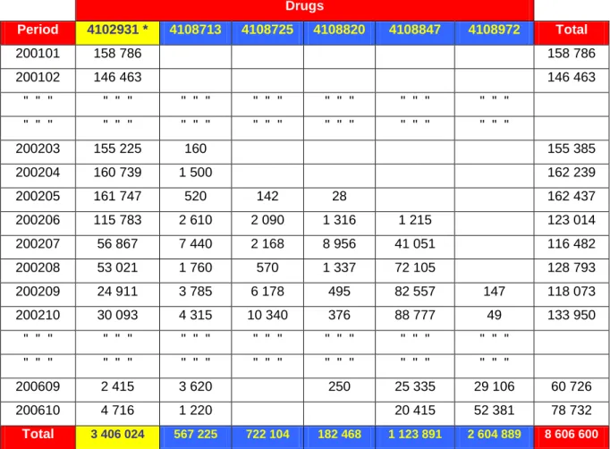
(13) My data cover pharmaceutical market representing the whole Västerbotten county of Sweden being both sparsely and densely populated. There are four inhabitants per square kilometre on average. The county Council of Västerbotten is one of the twenty one principal providers of medical care in Sweden. Aggregate data on the sales of Citalopram are provided by Apoteket AB. The dataset is detailed at product (Citalopram) / brand or generic code, i.g , N06AB04 4102931 , 41087713 etc. Since the aim of this study is to show how branded and generic version of Citalopram compete, I limited my analysis to the data set including a continuous branded and generic versions’ sales periods between September of 2002 and October of 2006. Thereby, six product were taken into account using the relevant literature of Anatomical Therapeutic Chemical (ATC) classification system. Table 1 : Data Summary Drugs Period. 4102931 *. 4108713. 4108725. 200101. 158 786. 158 786. 200102. 146 463. 146 463. " " ". " " ". " " ". " " ". " " ". " " ". " " ". " " ". " " ". " " ". " " ". " " ". " " ". " " ". 200203. 155 225. 160. 155 385. 200204. 160 739. 1 500. 162 239. 200205. 161 747. 520. 142. 28. 200206. 115 783. 2 610. 2 090. 1 316. 1 215. 123 014. 200207. 56 867. 7 440. 2 168. 8 956. 41 051. 116 482. 200208. 53 021. 1 760. 570. 1 337. 72 105. 128 793. 200209. 24 911. 3 785. 6 178. 495. 82 557. 147. 118 073. 200210. 30 093. 4 315. 10 340. 376. 88 777. 49. 133 950. " " ". " " ". " " ". " " ". " " ". " " ". " " ". " " ". " " ". " " ". " " ". " " ". " " ". " " ". 200609. 2 415. 3 620. 250. 25 335. 29 106. 60 726. 200610. 4 716. 1 220. 20 415. 52 381. 78 732. Total. 3 406 024. 567 225. 1 123 891. 2 604 889. 8 606 600. 722 104. 4108820. 182 468. 4108847. 4108972. Total. 162 437. Table 1 indicates a summary of the data in term of DDD (daily defined dose) used in this thesis, without time limitation on dataset. The first generic drug has been introduced into the market in March 2002 ,before the reform, and in September of 2002 one branded and 5. 13.

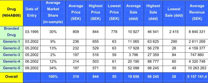
(14) generic product exist in the market. The drug having the code of 4102931, the branded version in the dataset, is the first product introduced into the market. We can see from the table that the generic-3, 4108820, is of very little use. Without any limitation on the dataset, the branded version’s sale is the highest one in the total consumption while the sum of two generics, ( 4th and 5th. generics), are much more than the branded version. In case of. limitation, changes in the sales are shown in table 2. It provides a list of the drugs, their prices and sales, included in the data set and existing in the Swedish pharmaceutical market. Table 2 : List of drugs, market shares, prices, sales and revenues Average Drug. Date of. Market. (N04AB06). Entry. Share. Drug. 03.1995. Highest. Lowest. Average. Highest. Lowest. Average. Price. Price. Price. Sale. Sale. (SEK). (SEK). (SEK). (ddd). (ddd). 30%. 809. 844. 778. 10 927. 46 541. 2 415. 8 840 331. (in-sample) Branded. Average. Sale (ddd). Revenue (SEK). Generic-1. 03.2002. 9%. 236. 655. 63. 11 065. 63 625. 290. 2 611 269. Generic-2. 05.2002. 13%. 232. 529. 63. 17 928. 56 278. 28. 4 159 377. Generic-3. 05.2002. 2%. 197. 516. 59. 3 796. 27 359. 84. 747 860. Generic-4. 06.2002. 12%. 214. 503. 61. 20 190. 88 777. 60. 4 320 748. Generic-5. 09.2002. 34%. 197. 571. 55. 52 098. 98 245. 49. 10 263 263. 100%. 319. 844. 55. 19 656. 98 245. 28. 5 157 141,4. Overall. Although there are some other branded and generic versions of Citalopram, I take these six products into account since others do not have continuous sales periods and some of them left the market during the study period. It is seen that the branded version which has entered into the market first and the generic 5 which has entered into the market last have the highest market shares, 30% and 34%, respectively. Even that the average sales of branded version is fifth in the market, it has second highest average market share and revenue, while it has the highest average price with low deviation between lowest and highest price compared to generic versions during the period.. In the figures 1 and 2 we can see the price and. consumption changes over the period.. 14.

(15) Price. Prices of branded and generic drugs over study period 900 800 700 600 500 400 300 200 100 0. Brand Generic-1 Generic-2 Generic-3 Generic-4 Generic-5 1. 4. 7. 10 13 16 19 22 25 28 31 34 37 40 43 46 49 Period. Figur 1 ( Price of branded and generic drugs). Quantity (ddd). Consumption of branded and generic drugs 50 45 40 35 30 25 20 15 10 5. 000 000 000 000 000 000 000 000 000 000. 000 000 000 000 000 000 000 000 000 000 0. Branded Drug Generics Total. 1. 4. 7. 10 13 16 19 22 25 28 31 34 37 40 43 46 49 52 Period. Figur 2 ( Consumption of branded and generic drugs). Figure 1 shows that although the overall consumption is decreasing ,the price of branded version is higher than the generics prices while its lowest, highest and average prices are 778, 844 and 809, respectively. Remember that the branded version has the second highest average market share and average revenue, thus, I conclude that the company producing the branded version believes that the consumers have a brand loyalty and it keeps the price high to benefit from this. As it is seen in the figure-1, prices of generics-1, 2 and 5 jumped in a some months. It is possible to derive some reasons from marketing strategies or from other terms. One of them could be that the firms agreed to increase the price or that they wanted to see if they could keep the price above the aggregate price. Figure 2 shows that the consumption is decreasing deeply. When I investigate the total consumption of excluded drugs before the start of the study period , it was almost 50 millions SEK, while the branded version’s consumption was more than 2 milliards SEK. Two of the excluded drugs left the market before the study period and the third drugs left the market after 15.

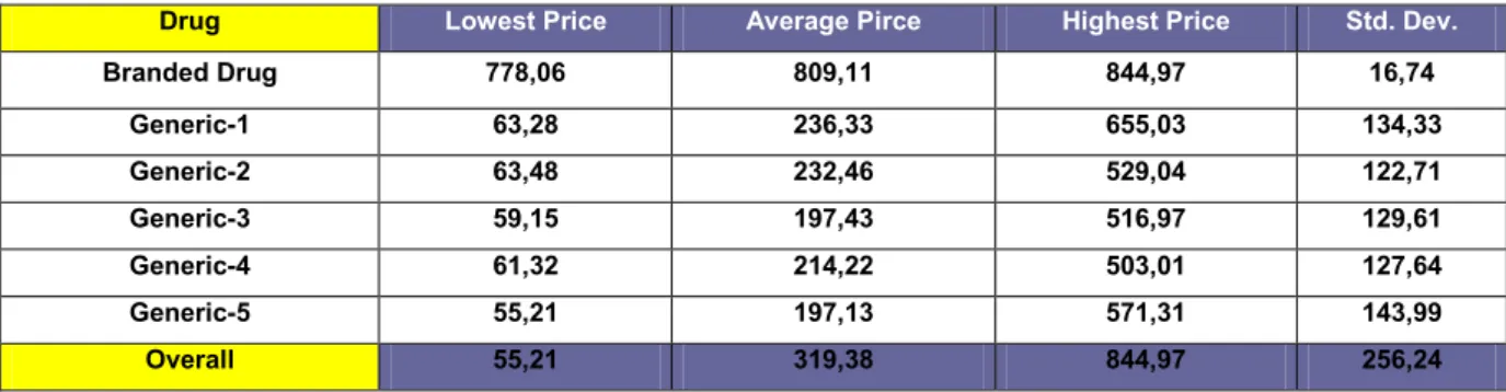
(16) 6 months when its total consumption was almost 47 millions. During the first six month, total consumption of drugs included in the data set is more than 413 millions SEK. Therefore, the decrease in the overall consumption is not directly related to the excluded drugs’ consumptions. Table 3 : Summary statistics of consumption Drug. Avr.DDD. Max.DDD. Min.DDD. Std.Dev.. Branded Drug. 10 927,48. 46 541,00. 2 415,00. 9 992,16. Generic-1. 11 064,70. 63 625,00. 290,00. 13 202,92. Generic-2. 17 928,35. 56 278,00. 28,00. 14 598,19. Generic-3. 3 796,24. 27 359,00. 84,00. 6 449,82. Generic-4. 20 190,41. 88 776,50. 60,00. 23 884,80. Generic-5. 52 097,78. 98 245,00. 49,00. 28 290,09. Overall. 19 656,08. 98,245. 28,00. 23 907,18. Table 4 : Summary statistic of revenue shares Drug. Avr.R.S. Max.R.S. Min.R.S.. Std.Dev.. Branded Drug. 0,30. 0,48. 0,14. 0,07. Generic-1. 0,09. 0,54. 0,00. 0,11. Generic-2. 0,13. 0,38. 0,00. 0,11. Generic-3. 0,02. 0,14. 0,00. 0,04. Generic-4. 0,12. 0,61. 0,00. 0,15. Generic-5. 0,35. 0,74. 0,00. 0,19. Overall. 0,18. 0,74. 0,00. 0,17. Table 5 : Summary statistics of prices Drug. Lowest Price. Average Pirce. Highest Price. Std. Dev.. Branded Drug. 778,06. 809,11. 844,97. 16,74. Generic-1. 63,28. 236,33. 655,03. 134,33. Generic-2. 63,48. 232,46. 529,04. 122,71. Generic-3. 59,15. 197,43. 516,97. 129,61. Generic-4. 61,32. 214,22. 503,01. 127,64. Generic-5. 55,21. 197,13. 571,31. 143,99. Overall. 55,21. 319,38. 844,97. 256,24. Tables 3 and 4 provide some sample statistics for the drugs observed in the data. It can be seen that the average revenue share of branded drug is higher than generic versions except for G5. Although the average sale of branded version in DDD ( daily defined dose) is the second lowest one, 10928 DDD, its revenue share is second highest one, 30%, since the company keep the price above the average price of generics. The generic-5, (G5), has the highest revenue share and sale. This may represent that generics versions of this drug can 16.

(17) compete directly with branded version for the market share after the end of the patent protection. On the other hand, table-5 shows that the branded version’s price is significantly higher than all generics’ prices in each period. Thus, it is possible to conclude that generics compete with the branded drug while they keep the price lower than the branded drug’s price. The branded version and fifth generic represent the highest and lowest average prices, respectively. This is very significant for the analysis since the total consumption of these two products accounts for almost 65% of the total expenditure. As I mentioned before, the twin objective of the Swedish Pharmaceutical Reform are to exchange expensive pharmaceuticals for cheaper generics, and increase the price competition. Until now, summary of data implied that the generic versions of Citalopram can compete directly with branded version for the market share after the brand owner has lost the patent protection. In following sections an empirical investigation of demand would show the degree of substitutability between these two types of product. 4.EMPIRICAL APPROACHES USED FOR DEMAND SYSTEMS 4.1.Multistage Demand System One of the central economic focuses of competition is the issue of “Differentiated products”. It is possible to find examples for this kind of products nearly in every market, like cereal, beer, toothpaste and pharmaceuticals. The common points for those products are of that the brand names are important because of costly R&D activities, and its heavy advertising. The importance of the structure of consumer preferences for the differentiated products was better understood through the advances in economic theory especially over the last two decades and empirical researches began to interest on this concept. Economists recognized that the results might be very sensitive to specific model assumptions on consumer preferences. Two models that are most widely used for consumer preferences in differentiated goods analysis are the representative consumer model or a model of different consumers with different tastes with symmetry property. The independence of irrelevant alternatives (IIA) is known as an axiom of decision theory and social sciences. If X is preferred to Y, then introducing an alternative Z can not make Y preferred to X. The structure of demand in those 17.

(18) models may be in conflict with the facts as the models have various features of IIA. This property was tested and rejected several times by the discrete choice literature, like Hausman and Wise (1978). Thus, it is needed to estimate a demand model which do not restrict unduly pattern of consumer preferences. Nowadays, transaction data are recorded in computers and available at the individual store level. However, one problem arise in use of the store level data. It is difficult to understand the estimation of a demand equation with large number of brands of a product. The multi-level demand estimation approach due to GORMAN (1971) solve this problem since it implies restrictions on demand pattern. This approach also allows for consideration of different segmentation patterns. GORMAN’s multi-stage budgeting approach (1971) is the basic approach which is useful in estimating demand for differentiated products in a three stage demand system. The top level corresponds to overall demand for the product. The middle level corresponds to different segments for the products which are used by marketing people in consideration of overall consumer preferences. The bottom level corresponds to competition within brands in a given segment. Estimating all three level and combining these estimates make able to calculate the overall own-and cross prices elasticities for each brand. This approach is widely used in estimation of demand systems since it is in accordance with segmentation of brand purchasing behaviour that marketing analysts claim rises in purchasing behaviour and it limits the number of cross elasticities. The top level equation corresponding the overall price elasticity is :. log ut   0  1 log yt   2 log  t  Z t    t (1) Where ut is overall consumption, yt is deflated disposable income, Πt is the deflated price index and Zt are variables which account for changes in some factors, like seasonal factors, demographics features. In the middle level the log-log demand system is used. k. log q mnt   m log y Bnt    k log  knt   mn   mnt (2) k 1. 18.

(19) m=1,...,M,. n=1,...,N. t=1,...,T. where the qmnt is log quantity of the mth segment in city n in period t, yBnt is total expenditure and the Πknt are the segment price indices for city n. Alternatives for the price indices are; a weighted average price index, Laspeyres type, Stone price index or some other price indices. However, the choice of the price index does not typically have much influence on the estimations. The econometric specification at the lowest level is the “Almost Ideal Demand System” of Deaton and Muelbauer. This model allows for a second order flexible demand system. The elasticities are unconstrained at the point of approximation. Using a flexible demand system make possible to set some restrictions on preferences when decreasing the number of unknown parameters through the use of symmetry and adding up restrictions from consumer theory. “For each brand within the market segment the demand specification is: J. sint   in   i log( yGnt / Pnt )    ij log p jnt   int (3) j 1. i=1,...J,. n=1,…,N. t=1,…,T. Where sint is the revenues share of total segment expenditure of the ith brand in period t in city n, yGnt is overall segment expenditure, Pnt is a price index and pjnt is the price of the jth brand in city n.”. [ Competitive Analysis with differentiated products, Hausman, Zona, Leonard 1994]. Test for βi=0 allows for a test of segment homotheticity, function of two or more variable in which the ratio of the partial derivatives depends only on the ratio of the variables, not their value; e.g., whether shares are independent of segment expenditure. The estimation of γij allows a free pattern of cross-price elasticities. The Slutsky symmetry can also be imposed by γij = γji . This does not impose any restrictions on competition within brands in a given segment. The use of segment expenditure, ygnt , rather than the use of overall expenditure is a very important econometric consideration since the overall expenditure is inconsistent with the multi-stage budgeting approach, and it can lead to certainly inferior econometric results.. 19.

(20) The next section gives more detailed information about the structure of the Almost Ideal Demand System. 4.2 Almost ideal demand system Estimation of demand for goods or services has been attracting the attention of both the business life and economists, thus, many other models had been proposed. Since Richard Stone’s first estimations of a demand system equations derived from consumer theory (1954), Linear expenditure system (LES) which has some limitations such as proportional income and price elasticities ,researchers have been continuing to work on alternative specifications and functional forms. Rotterdam model (Henri Theil, 1965,1976;Anton Barten) and the Translog model ( see Laurits Christensen, Dale Jorgensen, and Lawrence Lau; Jorgenson and Lau) are the most important ones in current use. In this study, I used the model, Almost Ideal Demand System (AIDS), due to Deaton and Muellbauer, that is of comparable generality of the Rotterdam and translog models, but which is more advantageous than both of them. It allows to compute income, own- and cross price elasticities using household survey data. This model gives an arbitrary first-order approximation to any demand system, satisfying the axioms of choice exactly. It aggregates perfectly over consumers without invoking parallel linear Engel curves. ( www.jstor.org/stable/1805222).. It is simple to. estimate since it avoids largely the need for nonlinear estimation. It has functional form which is consistent with known household-budget data. All of those advantages can be provided by other models, like Rotterdam and translog models. However the Almost Ideal Demand System possesses all of them simultaneously. “ Almost ideal demand system is to be recommended as a vehicle for testing , extending and improving conventional demand analysis.” (Deaton and Muellbauer, 1980) The beginning of demand system equations is the specification of a function that acts as a second-order approximation to any arbitrary direct or indirect utility function or, a cost function. The Almost Ideal Demand System use a first-order approximation to the demand function in term of generality, as the Rotterdam model do , but it starts from a specific class of preferences. Muellbauer (1975, 1976) argued that exact aggregation over consumers is possible within a specific family of preferences. These preferences are known as the PIGLOG. 20.

(21) class and it can be shown by a cost or expenditure function that is the minimum expenditure to achieve a certain level of utility at any given price.. log c(u, p)  (1  u) log ( p)  u logb( p) (1) Where u is the level of utility, which is between 0 and 1, α(p) and b(p) represent positive linearly homogeneous functions of a price vector p. Following Deaton and Muellbauer (1980) it is assumed that log a(p) and log b(p) are: log a( p)   0    k log p k  k. 1  2 k. . * kj. log p k log p j. j. (2). and. log b( p)  log a( p)   0  p k k k. (3). So that the Almost Ideal Demand System cost function is written as: log c(u, p)   0    k log pk  k. 1  2 k.  j. * jk. log pk log p j  u 0  pk k k. (4). Where αi , βi and γij* are parameters. It is possible to check that c(u,p) is linearly homogeneous in p, provided that the following restrictions on the parameters hold, in order to be a valid representation of preferences;.  i. i. 1 ;.  i. ij.   ij  0 ; j. . i. 0. i. We can derive the demand functions directly from equation (4) by applying the Shephard’s lemma and substituting afterwards indirect utility function that is derived form (2). The price derivatives are the quantities demanded :. pq  log c(u, p)  i i  wi (5)  log pi c(u, p) Where wi is the budget share of good i, that is given by the logarithmic differentiation of (4) as a function of prices and utility: 21.

(22) wi   i    ij log p j   i u 0  pkk (6) j. where,. 1 2.  ij  ( ij*   *ji ) (7) If we invert c(u,p), total expenditure x, for (4) and substitute into (6) to get u as a function of p and x, the indirect utility function, the AIDS demand function in budget share form can be denoted by:. wi   i    ij log p j   i log{ x / p}. (8). j. where P is a price index is defined by log P   0   k log pk  k. 1  2 j. . kj. log pk log p j (9). k. As seen in equation (9), the P term makes AIDS a nonlinear model. However, in the literature empiricists used a linear approximation for P quite often. The linear approximation most commonly employed is given by, which is known as Stone Price index; n. log P   wi log pi (10) i 1. The primary reason for the Almost Ideal Demand System to be used widely is that it can be approximated at the estimation stage by a linear form when it satisfies some of desirable properties. The Stone Price index is utilized since the linear model is not itself derived from a well-specified representation of preferences.. (http://www.allbusiness.com/marketing-. advertising/500617-1.html ) The following restrictions are implied by (4) and (7) : n.  i 1. i. 1.  i. ij.    ij  0 j. n.  i 1. i.  0  ij   ji (11). 22.

(23) Provided that (11) hold, the equation (8) denotes a function of demand system. These are homogeneous of degree zero in prices and total expenditure and satisfy Slutsky symmetry. The total expenditure is. w. i.  1.. The interpretation of the demand function summarized by (8) is straightforward. When there is not any changes in relative prices and real expenditures ( x / p ), i.e. the budget shares are constant. Predictions using the model start from this point. The terms γ ij affect the demand share when relative prices changes. These capture the effect on the ith budget share from a one percent increase in the price of the jth category of goods, with x/P held constant. Changes in real expenditure work through βi . The share equation exhibits also some basic properties of the demand function. Other things held constant, the expenditure share of each group of commodities is inversely related with its own price and positively related to the prices of other goods. Thus, it is expected that γii is negative. However, γij should have a positive sign for any i  j if goods are close substitutes. 4.3. Price elasticities In order to calculate elasticity estimates, it is needed to have time series data on prices. Note that data, from the Västerbotten County Council, that I used in this study are also in time series format. Now, in this section, I will explain the calculations of the elasticities. It is possible to derive the uncompensated ( Marshallian) own-price elasticities (εii) and cross-price elasticities (εij ) from the equations (10) and (8) as following ;.  ii  1 .  ij .  ij wi.  ii wi.  i.   i (12). wj wi. , i  j. (13). Where εii is the own price elasticity and εij indicates the cross-elasticity, in Marshallian (uncompensated) terms, wi is the budget share of good i, γii and γij are the coefficients of price. The Slutsky equation are very useful in the calculation for elasticity. We can derive the partial elasticity of substitution that is also known as the Allen elasticity of substitution. 23.

(24)  ij  w j ij  w j i (14)  ij  1 .  ij wi w j. , i  j. (15). Where σij is the Allen elasticity of substitution and the positive value implies that the two goods are substitutes or the negative value indicates that they are complements. 5.The MODEL for CITALOPRAM In this paper, I used a variant of the multistage budgeting model (Gorman, 1971), since it is in accordance with segmentation of brand purchasing behaviour. Drugs are grouped as branded and generics. In the model only one branded drug exists but there are five generics. Thus, the choice within the generics is conditional on choice of the generic group. Conceptually, the doctor prescribes a drug and patient use it but the reform in 2002 has made patients able to choose the cheaper one. This structure makes easier to estimate the own and cross-price elasticity of products. Data that I used is in panel data format, which is also called logitudinal data or crosssectional time series data. Below, in figure 3, you can see the product tree which is constructed to represent the two stage approach.. Figur 3 ( structure of the tree of Citalopram). 24.

(25) Conceptually, a consumer moves down the three. On the top model corresponding the choice of branded or generic version, almost ideal demand system is the specification which allows a flexible demand system specification. For the formulation of the model, there is need to calculate price index. In this study I used the Stone price index, as other similar studies did. On the bottom level of the tree, each node corresponds a generic drug. For example, the consumer can buy the prescribed branded or generic drug or as the reform imposes the pharmacy to inform whether there exist any cheaper substitutes, and he / she can choose one of the generics. The model consist two levels which correspond to the two-stage budgeting decision of the patient. He / she chooses one of the segments, branded drug, with the following equation: 5. Top level: st     log( rt / Px t )   b log( p B t )    g log Pgt trend t (16) g 1. Where st is the revenue share of the branded drug in time t, rt is the total consumption expenditure of drug, Pxt is the stone price index in time t, and defined as. log( Pxt )   j 1 s jn log( p jnt ) , where pjnt is the price of good j in city n ,in time t. PBt is the I. price of branded drug in time t, and Pgt is the price of five generics. Other right side variable is trendt which is a time trend. The bottom model correspond the consumer choices between five generic drugs. Each generic has an estimating equation. 5. Bottom: log q gt   g   log( Rt )    g log( p gt )  trend t (17) g 1. Where qgt is the quantity of generic g in time t , Rt is the total revenue of all generics in time t, pgt is the price of gth generic in time t, and trend t is a time trend. Note that there are five generics , hence , there are five equations.. 25.

(26) 6.ESTIMATION RESULTS 6.1.Estimation of Models The AIDS model defined by equation (16) and (17) is used to investigate the expenditure shares of branded version of Citalopram. The prices of generics, overall consumption expenditure, stone price index and the time trend are the independent variables. Explanatory variables are defined in natural logarithms, except for the trend variable. I estimated the model through the Ordinary Least Squares model , OLS, procedure by using STATA / SE 10.0 . In the dataset, two generics have zero sales in five periods. For instance, one of generics, 4108820, has zero sales in December of 2005, but before and after that time it has sales. This indicates that the product was still in the market but because of any reason, its sale was zero in the given time. Thus, they had likely a determined price. In order to have an appropriate result from estimations in STATA.10.0/SE I have estimated those months´ prices by taking the average prices of before and after that month prices. These predetermined prices make possible to use the Ordinary Least Squares method for calculating both models. It is possible to use different econometric methods. Here, I used the OLS method to present the equations. If the variable “P” in the equation 8 is known, the model would be linear in parameters α, β, and γ. The estimation can be done equation by equation by OLS, which, in this case and given normally distributed errors, is equivalent to maximum likelihood estimation for system as a whole. I model the choices at both levels similarly to Hausman, Leonard and Zona (1994). Remember that the top level describes the consumer’s choice between the branded and generic version. Table.6 shows the results of top level estimation.. 26.

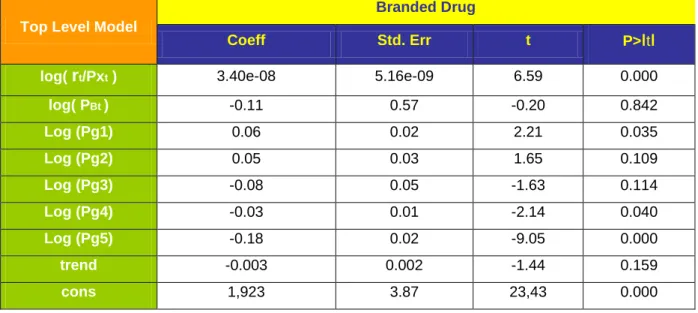
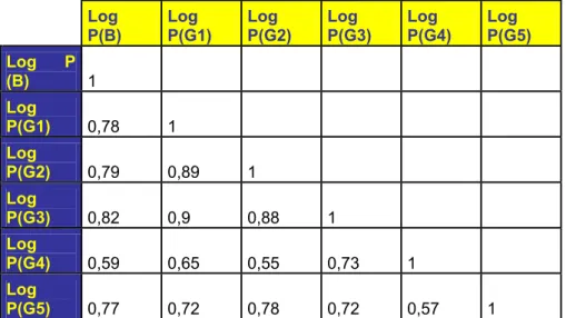
(27) Table 6 : Estimations for top level Branded Drug Top Level Model. Coeff. Std. Err. t. P>ιtι. log( rt/Pxt ). 3.40e-08. 5.16e-09. 6.59. 0.000. log( PBt ). -0.11. 0.57. -0.20. 0.842. Log (Pg1). 0.06. 0.02. 2.21. 0.035. Log (Pg2). 0.05. 0.03. 1.65. 0.109. Log (Pg3). -0.08. 0.05. -1.63. 0.114. Log (Pg4). -0.03. 0.01. -2.14. 0.040. Log (Pg5). -0.18. 0.02. -9.05. 0.000. trend. -0.003. 0.002. -1.44. 0.159. cons. 1,923. 3.87. 23,43. 0.000. The equation has been estimated with 40 observation. The adjusted R2 is 0.78 , indicating the model is able to explain the revenue share with 78% success. The F-statistic is reported as 18,76 which exceeds the critical value 2.25 and it shows that the coefficients are jointly significant. The effect of consumer expenditure log(rt /Pxt), divided by the price index, on the demand share of branded version is positive , significant at 5% , but close to zero. Moreover, we can not consider the sign of latter coefficient as a proof of inferior type of goods, since the dependent variable is not quantity, but it is the revenue share. The result of top level model for the branded drug and the results of bottom level model for each generic drugs which will be explained in this section indicate that drugs are normal goods since their price coefficients have negative signs as it was expected. Price coefficients do not seem so informative at this stage. Generics 1, 4 and 5 are significant at 5%. The own price coefficient of branded version is negative while the sign of generics 3, 4 and 5 are also, unexpectedly, negative. This result should not be interpreted immediately as a sign of complementarity rather than substitution with other version. Here, I tested if the coefficients of generics are equal, by using STATA. The null hypothesis is ; H0: log Pg1 = log Pg2 =…= log Pg5 The F-statistics is ; F(4,31)=24.35 indicates that the null hypothesis is rejected since the F-statistic exceed the critical value, 2,67 and we can conclude that these five generics have 27.

(28) different price coefficients. However, there is still need for more explication about the unexpected negative signs of three generics. Now, I shall interpret the correlation between branded and three generic drugs. The table 7 shows the correlation matrix of variables. Table 7 : Correlation Matrix Log P(B) Log (B). Log P(G1). Log P(G2). Log P(G3). Log P(G4). Log P(G5). P 1. Log P(G1). 0,78. 1. Log P(G2). 0,79. 0,89. 1. Log P(G3). 0,82. 0,9. 0,88. 1. Log P(G4). 0,59. 0,65. 0,55. 0,73. 1. Log P(G5). 0,77. 0,72. 0,78. 0,72. 0,57. 1. As it can be seen from the table above, there is a significant correlation between the price of branded drug and three generics. The positive signs reflect that values of both variables i.e, branded drug and generic-3, increase or decrease simultaneously. For instance, the value of 0.82 indicates a positive strong correlation between branded drug and generic-3. However, this can not be interpreted as a causality between two product. One interpretation could be that these products are produced by the same companies. “Following Stern (1996) and Feenstra (1995), the number of firms in the market could be an indicator of a changing competitive environment (Ellison, Cockburn, Griliches and Hausman 1997)”. As the market for Citalopram is a new market opened to producers of generic versions, there may be a insufficient competition and the company producing the branded version may have a strategy to acquire the highest revenue share by manufacturing generic versions under different names. Although the dataset used in the estimations does not include, there were three other branded drugs and two generics , which had been in the market for a short period. This could prove that the producer of the branded drug included in the dataset has a market strategy based on having the highest marker share and keep its rival away from the market by manufacturing generic versions beside the branded version and try to keep its market power as if it had still patent protection.. 28.

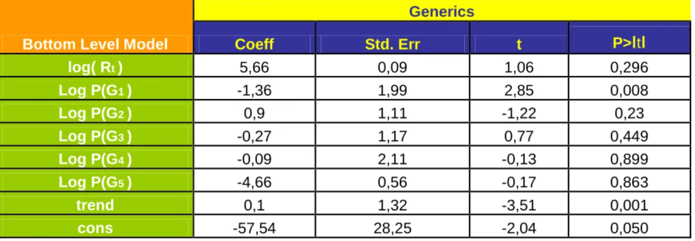
(29) The Allen elasticity shown in the table-10 represents the substitution and complementary relationship between the branded and generic drugs. It is suggested that positive values denote that those drugs are substitutes while the negative sign indicates the complementarity. The Allen elasticity of the branded version are , σ13 ,σ14 and σ15 , (-10.39), (7,13) and ( -0.70), respectively. Therefore, all these generics are complements for the branded drug. Now, I present the bottom level estimates. Here, the dependent variable is log quantity of generic drug i ( i=1,..,5) and the model describes how consumers substitute between different generics. Note that the equation is calculated for each five generics. Table 8 : Estimation of Bottom level model for Generic-5. Generics Bottom Level Model log( Rt ). Coeff. Std. Err. t. P>ιtι. 5,66. 0,09. 1,06. 0,296. Log P(G1 ) Log P(G2 ). -1,36 0,9. 1,99 1,11. 2,85 -1,22. 0,008 0,23. Log P(G3 ) Log P(G4 ). -0,27 -0,09. 1,17 2,11. 0,77 -0,13. 0,449 0,899. Log P(G5 ). -4,66. 0,56. -0,17. 0,863. trend cons. 0,1 -57,54. 1,32 28,25. -3,51 -2,04. 0,001 0,050. The Table 8 presents the result of the bottom level equation for the generic-5. The number of observation is again 40. Coefficients stands between the confidence interval. The F-statistic is given 5. 88 and exceeds the critical value, 2, 31. This implies that the log quantity demanded of generic-5 is related to explanatory variables in the model. The adjusted R2 is 0.46 , indicating the model is able to explain 46% success at the variation in the quantity demanded. The estimation gives unexpected negative signs for coefficients in this level also. The log price of generic-5 has negative sign, as it is expected. On the other hand, generic-1, 3 and 4 have also negative signs. When the correlation between these generics is checked , we can see that between generic-1 and 3 there is a strong positive correlation, that is shown in the Table 7. The positive sign of value represents that changes in log P(G1) and log P(G3) occurs simultaneously to the same direction.. 29.

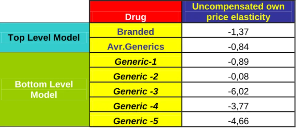
(30) As I mentioned before, in the top level estimation, one companies may produce two or more same drugs under different names in order to have higher market share in total, with respect to its marketing strategy. The calculation of elasticities will give us better explication about this. 6.2.Elasticities Using the results of the top level model estimation and by applying the definitions derived in section 4.3 , we can calculate the uncompensated own-price elasticities of the demand for six drugs. Table 9 summarises the calculations of own-price elasticity. Table 9 : Own Price Elasticities. Top Level Model. Bottom Level Model. Drug. Uncompensated own price elasticity. Branded. -1,37. Avr.Generics. -0,84. Generic-1. -0,89. Generic -2. -0,08. Generic -3. -6,02. Generic -4. -3,77. Generic -5. -4,66. All uncompensated own-price elasticities have the negative sign as there were expected and they vary between -6,02 and -0.08, substantially. When the price elasticity is analyzed , it is concerned with its absolute value, so we can ignore the negative sign. Thus, we conclude that the price elasticity of demand when the price increases one unit is 1,37 for the branded drug. The price elasticity of demand is used to see how sensitive the demand for a good is to a price change. The higher the price elasticity, the more sensitive consumers are to price changes. A high price elasticity suggests that when the price of a good goes up, consumers will buy a great deal less of it. The negative sign reflect that the demand is not sensitive to price changes. However, recall that the negative sign is ignored when analyzing price elasticity. Thus, the price elasticity of demand for branded drug is 1,37 and it is price elastic and sensitive to price changes. It is possible to conclude that the branded drug whose comparative advantage e.g. the patent protection, has been undermined by new alternatives. On the other hand, note that the generics 3, 4, and 5 are very sensitive to price when , in contrast, the generics 1 and 2 are relatively lower sensitive to price.. 30.

(31) The Allen elasticity whose result are reported in table 10 shows the substitution and complementary relationships between branded and generic drugs. Here, I used just the top level model, since I investigate the relationship between branded drug and generics. Positive values denote that those drugs are substitutes while the negative sign indicates the complementarity. Table 10 : Allen Elasticities Allen Elasticity Branded Generic-1 Generic-2 Generic-3 Generic-4 Generic-5. Branded 3,17 2,21 -10,39 -7,18 -0,7. Table 10 shows the Allen elasticities of six drug. In this case, generics having the negative sign appear to be complements for the branded version. Remember that the model estimations and the correlation table , table-7, had proved that there were a strong correlation between branded drug and these three generics. If these generics are not complements in practice, thus, I thing the suggestion is that the company of branded drug manufactures some other generic versions under different products names and it follows the same marketing strategy for all products that it produces. 6.3.Possible reasons for unexpected results The OLS regression has unexpected signs of some coefficients. For instance, in the top level estimation, the result implies that the revenue share of branded version increases with an decrease in its own price, while an increase in the prices of generic 1 and 2 rises its revenue share. However an increase in prices of generic 3, 4, and 5, lead the share of branded version to decrease. When we interpret this situation we can mention about some possible reasons. In general, it is expected that prices are correlated with the error terms since companies adjust prices to demand shocks. I assume that prices were predetermined with respect to the estimating equation. Preparing shelf stickers and some marketing material for stores may be a reason for doing this. This would be consistent with the structure of the retail chain. I observed also, in the dataset, that in a few months some drugs’ prices jumped up unexpectedly. If the supply reasons caused the price promotions, for instance a change in 31.

(32) input prices or shocks to inventory levels, then the price variation would not be correlated with the error term in the demand equations. Therefore, it is possible to assume predetermined prices with respect to the estimating equation, we can use OLS and identify parameters. In general cases, if prices are correlated with demand shocks , it is possible to classify into two levels. It is not expected that the demand shock in a given city affect price promotions significantly as the retailer prices multiple stores which are in the same district. In cases of that stores control the price, they can adjust prices to local demand shocks. On the other hand,. at the regional level, those shocks are taken into account by retailers and. producers arrange prices to vary according to the region that would violate the exogeneity assumption. One way to deal with this endogenous prices is to use the panel structure of the data to provide instruments. A possible instrument could be the pharmacy / hospital split. However, the dataset does not include sale in hospitals and it is not defined sales with respect to locations or cities in the dataset. The basic equations in my thesis are those of the model presented earlier with additive errors. I used the data set, monthly time series of price and revenue for six products. Note that each equation has not the same number of observation since the were some month for some of generics without sales. The current literature suggests that the dispensing doctors have a tendency to prescribe more medicines per capita than non-dispensing physicians (Trap et al. 2002). Dispensing doctors can be more risk averse and perceive a lower risk in prescribing new version of a drug. This could be a reason for the suggestion of that the company of the branded drug wants to keep its market power by manufacturing generic versions beside the branded version. Another reason could be related to the profit maximizing behaviour, since physicians get a mark up on directly dispensed drugs or pharmaceutical companies set effective marketing strategies. However, the Apoteket AB, managed by the Swedish government, provide the price to be the same in each counties. In addition, , there are not dispensing doctors in the Swedish health care system. Therefore, some other reasons must be investigated. One explanation might be that patients using the branded version may resist to substitute the drug that they use currently since they believe , wrongly, that any substitution would not show the same effect on their health. Remember that the County Council of Västerbotten is a regional foundation. Hence we can also expect that all generics may be not sold in every pharmacies and this may lead a wrong interpretation for the given drug in the model.. 32.

(33) The demand for Citalopram may be also affected by other variables rather than price which account for expenditure changes. For instance, the incidence of depressions may imply regional or seasonal trends in the per capita consumption. Socioeconomic characteristics of the population ,aspects of health care, life style may also affect the use of antidepressant drugs. However, all these aspects may have a little relevance in the demand share of different types of Citalopram, unless they shape preferences for specific product categories. The unexpected signs of coefficients lead to consider the concept of “endogenous variable”. It has causal links which lead to them from other variables or which has explicit causes within the model. If the prices for products are predetermined, the need for instruments is lower. Remember that because of months without sales but with determined prices before and after these months, I had assumed that prices were predetermined. The price endogeneity arises in estimating the demand functions when the price determination process includes significant interplay of supply and demand. In the demand models, the price is endogenous since consumers can change their demand in response to the price. We can mention about endogeneity when parameters or variables are predicted by other variables in the model. The independent variables in the top level and bottom level models, the revenue share and the quantity demanded, respectively, may be correlated with the error term. For the demand of Citalopram, we can not mention about consumer tastes since it is the physicians who prescribe the drug. On the other hand, consumer preferences are more effective in the decision making process with respect to the Swedish pharmaceutical reform permitting them to choose the lowest priced drug. Besides the price, the expenditure can also be an endogeneity problem. A demand analysis can not cover all goods and services that a consumer purchases. Such analyses indicates the last stage of a multi-stage budgeting process which is justified on the assumption of weak separability of preferences ( Deaton and Muellbauer 1980). Therefore, when the consumer expenditure allocation is correlated with the demand behaviour of the product or product group being analyzed , expenditure endogeneity may arise. This endogeneity problems arise when there are some factors effecting the consumer choices that are not taken into consideration by the model , dataset or the researcher. In contrast with the Swedish pharmaceutical market, it is possible to derive some reasons from the marketing or pricing strategies of retailer companies in other countries. The price is. 33.

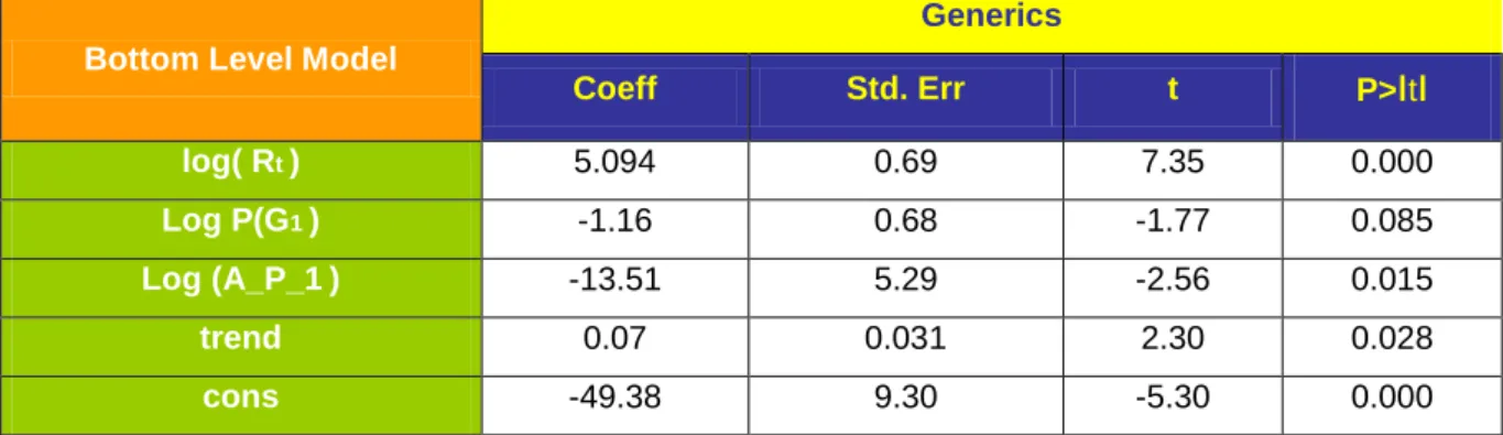
(34) determined according to the price strategy incorporating supply and demand characteristics. If some of the determinants of the pricing process include unobserved demand characteristics, considering the price as exogenous, leads to biased and inconsistent demand estimations. The same possible reasons, e.g, unobserved factors, are in valid for the expenditure endogeneity also. However, as I mentioned before, the Apoteket AB provides the price to be same in each county. The instrumental variable estimation method is a way to control for price endogeneity. For instance, Hausmand, Leonard and Zona and Nevo (2001) has used an instrumental variable approach first proposed by Hausmand and Taylor for panel data. Another alternative approach includes the explicit specification of price equations which reflect strategic firm behaviour. The first approach takes advantage of the panel nature of multi-city scanner data and it uses the prices of neighbouring cities as instruments. The second approach , instruments for estimation are the demand and supply shifters within a city or region. One possible instrumental variable could be the pharmacy / hospital split, however , the dataset contains sales only in pharmacies. To test if the model is mis-specified ,I applied the “Ramsey Reset Test” for the top level model and the F-statistic is reported as 3.75 . It exceeds the critical value of 2.94 . But the value of “Prob>F”=0.022 and this implies that we should better not to be sure that the null hypothesis is rejected. The result of the bottom level for the first generic denote that there is one or more omitted variables. The F-statistic is 1.90 and lower than the critical value, 2.93. Therefore, it is obvious that both model can be developed by more explanatory variable(s). In order to reduce the endogeneity in the model by using the current dataset, it is possible to use one variable that may be called “log average price of generics “ (Log_Average_P_G) instead of five “log price” variables. Because the endogeneity rises when parameters or variables are predicted by other variables in the model. By using the average price, I aimed to reduce possible direct relationship between parameters or variables. Remember that the Allen elasticity in section 6.2 has implied that the branded drug and the generics 3, 4 and 5 are not substitutes. For the top level, estimations is shown in table 11. Coefficients have still unexpected sign . The adjusted R2 , 0.19, and the F-statistic decreased to 3.31. It is still significant but not more than the original model.. 34.

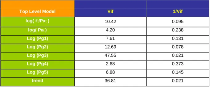
(35) Table 11 : Estimation of top level with Log ( Average Price of Generics ) Branded Drug Top Level Model. Coeff. Std. Err. t. P>ιtι. log( rt/Pxt ). 5.93e-09. 8.20e-09. 0.72. 0.474. log( PBt ). -0.58. 1.07. -0.54. 0.59. Log (A_P_G). -0.08. 0.05. -1.50. 0.141. trend. -0,005. 0,002. -2.24. 0.031. cons. 4.70. 7.11. 0.66. 0.513. For the bottom level model, each generics have an estimation. Here, I calculated the model just for the first generic by using a variable called “L_avr_price1” which indicates the average price of generics other than the first generic’s price. The result is reported in the table 12. In this case, the adjusted R2 is lower, 0.69, and the F-statistic, 20.12, is almost the same with the original model. All of the coefficients would become significant at α =0.10 . Thus, it is possible to use the “log average price” variable rather than four log price variables of generics other than the first generic, in order to reduce the endogeneity. Estimation with the same way for other generics are reported in appendix. Table 12 : Estimation of bottom level model for generic-1 with log average price Generics Bottom Level Model. Coeff. Std. Err. t. P>ιtι. log( Rt ). 5.094. 0.69. 7.35. 0.000. Log P(G1 ). -1.16. 0.68. -1.77. 0.085. Log (A_P_1 ). -13.51. 5.29. -2.56. 0.015. trend. 0.07. 0.031. 2.30. 0.028. cons. -49.38. 9.30. -5.30. 0.000. Another possible reason for unexpected sign may be multicollinearity problem which corresponds the dependencies between the dependent variable and independent variables. As it is shown in the section 6.1, between some of generics and the branded drug there is a relation other than the substitution and this causes some variables to be the components of a mixture. Although the F-statistics of models are significant, it is possible to have multicollinearity when the individual regression coefficients are not significant. Thus, I checked it by the “Variance Inflation Factors”. It is suggested that the larger the variance inflation factor is, the more severe the multicollinearity will be. 35.

(36) Table 13 : Results of Vif. Top Level Model. Vif. 1/Vif. log( rt/Pxt ). 10.42. 0.095. log( PBt ). 4.20. 0.238. Log (Pg1). 7.61. 0.131. Log (Pg2). 12.69. 0.078. Log (Pg3). 47.55. 0.021. Log (Pg4). 2.68. 0.373. Log (Pg5). 6.88. 0.145. trend. 36.81. 0.021. The Table 13 shows the STATA output of the variance inflation factors for the top level model. It is argued that if it is more than 10, there exist multicollinearity problem. The mean of variance inflation factor is reported as 16.11 while four of regressors also exceed 10. Thus, it is clear that there exist multicollinearity problem. One way to eliminate or reduce this problem could be using a method which is less sensitive to multicollinearity than ordinary least squares e.g. ridge regression. Another alternative is augmenting the data with new observation specifically designed to break up the approximate linear dependencies that currently exist.. 36.

(37) 7.CONCLUSION The demand systems are one of the central economic focuses of competition. After the reform in the Swedish pharmaceutical market, the focus on the demand of drugs without patent protection become more important in order to reduce the health care expenditures and increase the price sensitivity of the market. I proposed a model of demand for Citalopram in this thesis. The estimations indicated that the linear approximate almost ideal demand system model can be improved by determinants of demand structure other than price, like a regional, demographic, cultural characteristics of the County of Västerbotten or by diversification of sales with respect to the sales in hospitals and pharmacies. Additional variables can make the model more appropriate. In contrast to the general expectation on new entries to a market, in the pharmaceutical market, the price of the branded drug, usually, is not effected dramatically and does not jump down immediately. It can be considered as an evidence that the price deviation is not high for the branded drug. One demand side feature of the branded version is that price discounts after the end of the patent protection and the price competition increased through the reform do not have much effect as it might be expected. New entries of generics decreased the demand and the price of branded drug, however , it has still highest second revenue share. The uncompensated elasticity of the generic-2 is relatively inelastic, (-0.08), and it implies that the quantity demanded changes less than the change in price, while the generic-1 is near the unit elasticity, (-0,89). These values are smaller than the other generics’ own price elasticities and the branded drug’s. I found high correlation between the prices of branded drug and three generics, in addition, the Allen elasticity showed that they are not substitutes. Thus, I concluded that the generics-1 and 2 , with almost %23 of revenue share in total, are able to compete in the market that can be considered as a new market if they keep the their price lower than the branded drug’s price. As the Allen elasticities denote, the branded version and three generics are complements. It is argued that companies may have different names strategy since selling of generic equivalent that for 50% to 80% less than the cost of the brand name (www.whocc.no/atcddd/). The role of the reform can be separately a topic to study, however, I think that more effective dissemination of information on prices might be an example of measure to improve. 37.

(38) efficiency in the use of pharmaceuticals in such a country like Sweden, having high health care expenditure. Finally, a common difficulty in the estimation of demand function is the lack data which is at a local level and is not easily available. I think that it would be advisable to promote the regular collection and they can be used in new studies. Obviously , the results of this kind of partial analysis may not be very reliable for a marketing researcher to design a policy. Deaton (1988) has introduced an approach for using household survey data in order to calculate the price elasticities. However, its application needs certain conditions on the data set which can not always be met.. 38.

No results found