A method to generate drive cycles from operational data

(1)

IN

DEGREE PROJECT

VEHICLE ENGINEERING,

SECOND CYCLE, 30 CREDITS

,

STOCKHOLM SWEDEN 2019

A method to generate drive

cycles from operational data

DAVID AKNER

KTH ROYAL INSTITUTE OF TECHNOLOGY

SCHOOL OF ENGINEERING SCIENCES

(2)

(3)

iii

Abstract

This thesis investigates the possibility to develop a method to generate drive cycles for heavy duty vehicles for Scania’s customers. A representative drive cycle is important to simulate realistic driving of vehicles.

Trucks that are sold by Scania and other manufacturers are collecting data which are logged from the vehicle’s on-board computer during operations. This data is used for the development of new trucks, and the idea is that with operational data, a drive cycle can be generated which is representative for the operations of a specific truck.

The developed methodology generates a drive cycle which is compared against this operational data. By making a first selection of already existing drive cycles and modifying the closest drive cycle to a selection of parameters, a drive cycle which corresponds to the operations of the specific truck can be designed.

To compare against the operational data, simulations of the truck performing the drive cycle are conducted, and the results are compared to the truck’s operational data. The simulation tool is an internally developed model at Scania which has been verified against test measurements on trucks.

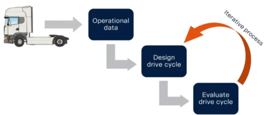
A final methodology to generate drive cycles are developed and it compares the simulated fuel consumption and engine load matrix against operational data. By redesigning the drive cycle in an iterative process, results from simulation of the drive cycle becomes very similar to the operational data.

(4)

(5)

v

Sammanfattning

Detta examensarbete undersöker möjligheten att utveckla en metod för att generera körcykler för tunga vägfordon för Scanias kunder. En körcykel som är representativ mot verklig körning är av stor vikt för att ha möjligheten att kunna simulera en realistisk körning av vägfordon.

Lastbilar som säljs av Scania och andra fordonstillverkare samlar in kördata som loggas på fordonets interna dator under användning. Dessa data används i vidareutvecklingen av fordon och idén till detta arbete är att med tillgänglig kördata kan körcykler genereras som efterliknar användningen av en specifik lastbil.

Den framtagna metoden tar fram en körcykel som jämförs mot kördata. Genom att först välja ut en redan befintlig körcykel som generar liknande resultat sett till kördatan så kan denna körcykel designas om för att än bättre anpassas till kördatan.

Genom simulering kan körcykeln testas med det fordon som körcykeln skall efterlikna. Resultaten från simuleringen av körcykeln jämförs med den loggade kördatan. Simuleringsverktyget har utvecklats internt på Scania och är verifierat mot tester från lastbilar som genomfört verkliga körningar.

Den slutgiltiga metoden som genererar körcykler jämför bränsleförbrukning och motorns lastmatris jämtemot den loggade kördatan. Genom omarbetning av körcykeln i en iterativ process tas en slutgiltig körcykel fram som ger ett mycket liknande resultat mellan simulering och loggad kördata.

(6)

(7)

vii

Preface

As this is the last work that I will perform in my engineering master degree I hope to be able to achieve a work which somewhat contributes to the development of real products. In the vehicle industry, scandals of cheating test cycles have been a big topic during the time of my studies. I hope that the methodology developed and suggested in this report can be of use to give accurate simulation results which might provide a higher standard in HDV development.

I am truly grateful for all the professional support I’ve received while performing this work. My supervisors Antonius Kies and Anders Jensen from Scania has offered me many giving advices. The support that I’ve received from my supervisor Jenny Jerrelind at KTH has been very helpful to achieve a report which is well written and clear. I would also like to thank my other colleagues at Scania for giving me a good time and learning me interesting things while performing this work. Last and not least, I’ld like to thank my family and friends for giving me support and encouragement throughout my studies, without you this would have been much harder!

(8)

(9)

ix

1. Introduction

Today there are large needs to transport goods and people all around the world. Different transport needs require different transportation modes. When it comes to transporting goods on land such as food, clothes, electronics and other supplies, trucks account for about 70% of all road freight. A total of roughly 400 000 trucks were manufactured in Europe in 2016, and continuous development by the manufacturers is a necessity to reduce the environmental impact and improve the usability in order to maintain or increase the company’s market share [1].

Scania is a manufacturer of commercial vehicles and engines, mainly within heavy trucks and buses. The company has been developing trucks and buses for over 100 years and employs today almost 50 000 people worldwide of which about 4000 are within research and development [2].

For Scania, the development of trucks is continuously ongoing and an important tool in the development is the possibility to analyse operational data. Scania trucks sold since 2011 gather and upload operational data to Scania’s research and development facilities. Today more than 350 000 vehicles are connected [3]. With this data, Scania can develop tailor-made solutions for its customers which are based on how the sold trucks are driven by the drivers on real roads.

To test vehicles, there are different drive cycles that the vehicle can perform. A drive cycle is a series of data points which tells the speed and gradient that a vehicle should perform. When an engineer has a drive cycle, it is possible to either simulate or test the vehicle physically with either real driving or having it run on a so called chassis dynamometer, also known as a rolling road [4]. In order to make sure that the drive cycle accurately reflects real driving, it is necessary that the drive cycle is based on some real driving pattern.

1.1. Purpose of thesis

The aim with this work is to develop a method where drive cycles can be generated for a specific truck with available operational data. The methodology should be general so that it can be applied to different sorts of trucks. The drive cycles will be validated through a simulation tool using longitudinal vehicle dynamics.

More specifically, the goal is to generate drive cycles which represent fuel consumption and engine work accurately whilst having a similar topography and vehicle speeds as the underlying operational data.

1.2. Delimitations of thesis

The thesis is limited mainly by the time constraint which is 20 weeks of work. In order to manage this time constraint and limit the work further, the thesis will not include making any validation of how well the methodology generates a drive cycle. That is, to not investigate with real measurements how accurately the drive cycle fits the operational data. Furthermore, there will be a selection of parameters in the operational data that will be used in the design process. Too many parameters used for comparison was argued to be too time consuming for this time frame.

(12)

2

1.3. Work plan

The following work plan was set up at the beginning of the work in order to reach the final goal of having a methodology to generate drive cycles from operational data.

a) Literature survey on:

• Representing real driving with drive cycles • Theory to generate drive cycles

• What data is used in the design of drive cycles

• Differences between passenger cars and heavy duty vehicles b) Investigation of available operational data in order to understand:

• What sort of data that is available

• Which parameters should be extracted and used

c) Development of tools to compare simulation and operational data • Learn and understand the simulation model that will be used • Develop scripts which analyse drive cycles statistically

• Develop scripts which compare simulated results and operational data d) Evaluation of results and development a method for generating drive cycles

• Does simulated results reflect operational data well? • Should any comparable parameters be changed? • Make graphs and tables easy to compare

e) Generate a drive cycle for the customer value vehicle with the method

1.4. Outline of thesis report

The thesis report will start with a short background (Chapter 2) on relevant topics to the work. Thereafter a chapter describing the theory (Chapter 3) related to generating drive cycles as well as theory to the simulation model used. In Chapter 4, the developed methodology is presented and explained followed by Chapter 5, presentation of the results to a generated drive cycle for the customer value vehicle. The final part of the report is some discussion and conclusions, as well as some indication of future work.

(13)

3

2. Background

2.1. Research and development at Scania

The main segment of Scania are long haulage trucks which consist of a tractor and a trailer which transports goods over large distances. Scania trucks are today sold within all continents of the world and the trucks perform different driving patterns in different parts of the world. In order to develop trucks which are adapted around the specific customer, Scania offers a customisation of each truck where for example different engines can match with different gearboxes.

In order for Scania to develop trucks that are performing well for all its markets, it’s important that the engineers have a good reference how the vehicles are driven in different parts of the world. Therefore, many different drive cycles must be used to reflect the driving patterns in different segments and different countries. With the ability to collect data from a specific truck anywhere in the world, it should be possible to have a drive cycle which reflects the driving of that truck.

There are two main types of trucks. Articulated trucks have a tractor which pulls a semitrailer on a fifth wheel. This type is usually used for long haulage applications. The other type is the rigid truck where the full truck, including its cargo bay are mounted on a common frame.

2.2. Operational data

As mentioned earlier, all trucks sold by Scania are equipped with a communication system which sends the operational data to Scania. The operational data contains many different parameters which partially reveal how the specific truck is being driven. However, the data is not time resolved but rather collected as aggregated data to show the vehicles performance in general. Examples of operational data parameters are average moving speed, distribution of the road slope driven by the vehicle and how many stops that are performed per 100 km.

By combining different parameters from the operational data, it is possible for the engineers to extend this information and understand how the truck is driven. For example, the combination of speed and gradient distribution as well as engine loads could reveal if the specific truck is equipped with a too small engine for the sort of driving that the vehicle is performing. This would be the case if the engine operates mainly at full load.

2.3. Drive cycles

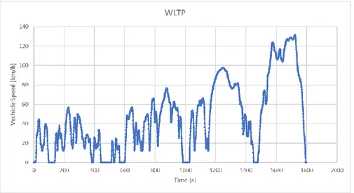
Drive cycles are used to assess a vehicles performance in regard to areas such as emissions, fuel consumption or powertrain performance. A cycle is a set of datapoints which tells how fast and with what slope a vehicle should drive, at a specific time or distance. Below is an example of the WLTP (Worldwide Harmonised Light vehicle Test Procedure) [5] which is used to benchmark passenger cars’ emissions and fuel consumption. This cycle is the common cycle in EU which all new passenger cars needs to be tested against, it is aimed to reflect typical driving of passenger cars. The passenger car cycles are used here as examples since they are more well known among the common audience.

(14)

4

Figure 1. The drive cycle WLTP used to test passenger cars.

Usually, drive cycles are developed by national authorities or organisations to have a common way for all manufacturers to test their vehicles and thereby compare the vehicles with each other. However, many road vehicle manufacturers have developed their own drive cycles to better reflect their main segments. This is done because drive cycles represent different sorts of driving and it is important when developing a new vehicle that the benchmark drive cycle accurately reflects the real world driving pattern.

A problem which arises from these common benchmarking drive cycles is called “cycle beating”, where manufacturers have designed their vehicles to operate best when performing a specific drive cycle, so that the performance indicators show that their vehicle is optimal. The issue is that the drive cycle only reflects one sort of driving which is not representative to all types of vehicles and drive patterns. For example, previously the NEDC (New European Driving Cycle) [5] has been used to assess passenger cars’ performance but has been criticized of misrepresenting real driving accurately. As shown in a report from the International Council on Clean Transportation [6], the NEDC cycle misrepresent passenger cars’ fuel consumption with up to 20 % compared to real fuel consumption. Therefore, it is important to have drive cycles which accurately reflects real driving patterns of vehicles.

When developing the cycles, it can be done either theoretically with set speed, acceleration and gradient, or the cycle can be the exact measurement from driving. Both ways of designing the drive cycle originates from real driving. By analysing the data from real driving and considering ambient conditions such as weather, traffic and road condition, it’s possible to say that a certain measurement of this driving represents a specific type of driving such as, urban, rural or highway driving.

2.4. Customer Value Vehicle, CVV

In order to have a vehicle that represents the typical customer at Scania, the company has developed a method to pinpoint a specific vehicle which on average represents the typical Scania customer operation within a certain transport application. This typical truck is called a Customer Value Vehicle, (CVV) and has a specific chassis number with a unique component specification. The truck itself is rolling on public roads in real traffic and is used by its operator.

(15)

5

For this thesis, the Customer Value Vehicle which represents Scania’s main segment, long haulage trucks, is used to develop the methodology of generating drive cycles. The final drive cycle therefore aims to represent the drive patterns of this specific truck. The specifications of this Customer Value Vehicle, denoted as CVV1, is specified in Table 1 below. Since the truck is in operation at a customer, it cannot be used for testing or validation purposes at Scania’s facilities.

Table 1. Specifications of CVV1.

Type Tractor 4x2

Application Long Haulage

Engine 13L - 6 cyl. - 450 HP - EU6 Gearbox 12 speed AMT, 11.32 - 1.00 Axle Gear Single reduction axle, 2.59

Wheels 315/70 R22.5

Average vehicle mass 26.79 tons

2.5. Vehicle simulation model

In order to simulate the drive cycles, a vehicle model developed at Scania has been used. The model itself uses the same approach of simulations as done in VECTO, Vehicle Energy

Calculation Tool [7]. VECTO is a tool developed to determine CO2 emissions and fuel

consumption of Heavy Duty Vehicles, HDV. The definition of Heavy Duty Vehicles are vehicles with a gross vehicle weight of more than 3.5 tons. The Scania vehicle model was developed by Johan Holmberg [8] as part of his master thesis.

Since 1st_{of January 2019, the VECTO tool is mandatory for vehicle certification for all OEMs}

whose vehicles are considered in the CO2 legislation. The tool uses data that is specific for

all relevant components, for example masses, friction, inertias, auxiliary powers and engine efficiency. The results from VECTO are thus unique for each combination of components and give a relevant measure of the fuel consumed and the CO2 emitted for a specific vehicle

(16)

6

3. Theory

The purpose of this chapter is to give relevant background theory on how drive cycles are designed. The latter part of the chapter aims to present the theory on how to simulate drive cycles with longitudinal vehicle dynamics and also give theory for engine load matrices.

3.1. Drive cycles

A drive cycle is a set of datapoints which show how a vehicle should operate over a set of time or distance. The datapoints can describe what speed or gradient that the vehicle should operate at.

The drive cycles’ speed profile is generally divided into two sorts; target or demanded velocity profiles. Target velocity cycles are cycles where the speed of the vehicle should reach a certain target with no set constraints for the acceleration. For demanded velocity cycles, a targeted speed should be achieved but the acceleration is set by predefined limits, meaning that the drive cycle sets the bound on what maximum accelerations are allowed.

As mentioned before, the speed and gradient profiles are based either on time or distance. In Figure 2, an example of a distance based drive cycles with targeted speed (orange) and demanded speed (blue). Note how the demanded speed profile has a limited acceleration.

Figure 2. Generic distance based drive cycle showing target and actual vehicle speed [8].

3.1.1. Transient or setpoint cycles

For the layout of cycles, there are two distinct types. Either you have a transient pattern of the cycle such as the WHVC (World Harmonized Vehicle Cycle) cycle [5], or the cycle can be made up of set points for certain durations with constant accelerations. An example of set point cycles are the SORT (Standardized On Road Test) cycles [5]. Transient and set point drive cycles are two different types of representing drive patterns. Figure 3 and Figure 4 shows the two different types.

(17)

7

Figure 3. The WHVC cycle is an example of a set point cycle.

Figure 4. The SORT 3 cycle is an example of a set point cycle.

3.1.2. Comparable parameters for representing real driving

In order to link a certain driving pattern with a drive cycle, the driving must be quantified. Depending on the usage of the drive cycle, different parameters will have a higher impact on the output than other parameters. In the case of developing drive cycles which are supposed to more accurately reflect the fuel consumption for real driving, there are certain parameters that have a higher significance relating to the fuel consumption when performing the drive cycle.

Studies which have been performed to quantify the parameters that influence fuel consumption the most has generally been done by comparing vehicles driving in many different driving patterns whilst collecting data. With factorial analysis, linking the properties between each vehicle and its fuel consumption, a selection of parameters with the highest influence was made as done by Ericsson’s research [9]. These parameters, also called characteristic parameters can be categorized into different parts of driving patterns. These groups, Dynamics, Operation modes, Speed and Acceleration, have several characteristic parameters within them.

(18)

8

Dynamics describe how the changes in driving occur, how much power is needed to

accelerate in different levels, usually grouped in low, medium and high power levels. The

Operation modes describe how often and for how long different driving scenarios such as

stopping, cruising and accelerations are occurring. Speed parameters describe the distribution of speed as well as what the mean and maximum speeds are. Acceleration parameters, include positive and negative accelerations and are usually set by certain limits stating how often acceleration occurs above or below a certain limit. The specific characteristic parameters for these groups are collected during driving and are then used later in the design phases [10].

From the report by Ericsson [9] some of the most important characteristic parameters are summarized in Table 2. These parameters are for example also used by Huertas and others [10], in their methodology.

Table 2. Summary of most occurring parameters linking drive patterns to fuel consumption.

Group

Parameter

Dynamics Acceleration power factor*

Stops per 100 km Operation modes Percentage idling Percentage accelerating Percentage decelerating Percentage cruising Speed Average speed Standard deviation speed

Maximum speed Speed distribution

Acceleration

Average acceleration Average deceleration Standard deviation acceleration Standard deviation deceleration

Maximum acceleration Maximum deceleration

*) The acceleration power factor is a measure of how much time is spent in

different levels of power usage, usually high, moderate or low power. This gives a good indication as to how “aggressive” the accelerations are.

3.1.3. How drive cycles can be designed

Most drive cycles are usually based upon data collected from driving in traffic. The collected data can thus be impacted by the driver’s unique drive style, traffic specific circumstances and other non-controllable parameters. When collecting data in real traffic, there should be different drivers driving in different patterns with varying traffic conditions to mitigate the risk of having misrepresented data that is used to generate a drive cycle.

From the collected data, there are different ways of generating a drive cycle. Two ways that are occurring more often in literature are mathematical design with Markov chains and

(19)

9

Monte Carlo methods as described further in Huertas report [10]. The other way is iteration of a drive cycle until the design has similar characteristics as the data collected from all drive patterns. The method using iterations is chosen in for the work in this thesis.

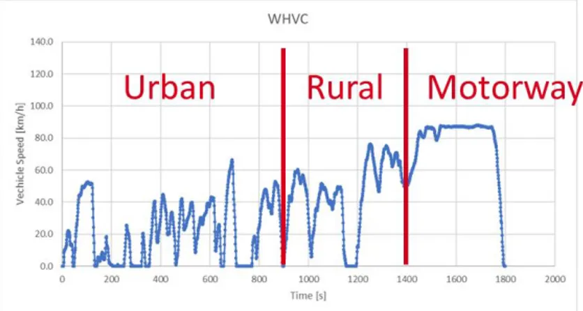
To iterate a drive cycle which yields the same characteristic parameters as the collected data, it can be done in two ways. The designer can make a set point cycle or can use parts of collected data to form a full cycle. A set point cycle sets the duration and magnitude of accelerations and speeds. These set accelerations and speeds will affect the parameters within dynamics and operational modes which again is compared to the collected data. This methodology was done when designing the SORT cycles [11]. Another way to perform iterations for a drive cycle, is by combining different base cycles which together form a complete cycle which better fits the collected data. As described in the SORT report, this can create as many drive cycles as there are drive patterns. The idea is that some base cycles represent different driving patterns and by combining these you will change the characteristic properties related to your collected data. As shown below in Figure 5, the WHVC cycle for heavy duty vehicles, used this approach to create the cycle which consists of urban, rural and motorway driving parts [5]. The approach with base cycles is independent of having transient or static, set point layouts.

Figure 5. The WHVC cycle consists of different base cycles.

3.2. Simulation of drive cycle

In order to simulate the drive cycle, the thesis used a vehicle simulation model developed at Scania by Johan Holmberg [8]. The model itself is built up in Simulink, a graphical coding program within MATLAB and the model has been validated against real measurements. The Simulation model is based on longitudinal vehicle dynamics and can simulate the performance of a truck performing a drive cycle. Below follows a description of the vehicle model and the simulation environment for the driving cycles.

3.2.1. Longitudinal vehicle dynamics

Longitudinal vehicle dynamics are the modelling of a vehicle travelling in the longitudinal direction. With the simplification that the whole vehicle consists of rigid bodies without any elasticity and deformation, equations relating the vehicles acceleration to the forces acting on the vehicle when travelling. Antonius Kies shows in his report [12] what forces that acts on a wheeled vehicle shown in Figure 6.

(20)

10

Figure 6. Forces that act on the vehicle in the longitudinal direction [12].

With Newtons 2nd_{law and equilibrium of forces, an expression for the required wheel force}

to overcome other longitudinal forces can be acquired and is shown in Equation 1.

𝐹𝑤ℎ= 𝐹𝑟𝑜𝑙𝑙+ 𝐹𝑔𝑟𝑎𝑑𝑒+ 𝐹𝑎𝑖𝑟+ (𝐹𝑖𝑛𝑒𝑟𝑡,𝑡𝑟𝑎𝑛𝑠𝑙+ 𝐹𝑖𝑛𝑒𝑟𝑡,𝑤ℎ) (1)

Where: Fwh Tractive forces at the wheels Froll Rolling resistance forces of tires Fgrade Gravitational forces acting on vehicle Fair Air drag force acting on vehicle

Finert,transl Inertia force of translationally accelerated vehicle mass Finert,wh Equivalent inertia force of all rotating wheels

Through simplifications and assuming small road angles and no cross-wind, the equation can be rewritten into Equation 2, where a more complete expression declares what forces act on the vehicle.

𝐹𝑤ℎ= ( ∆𝑎𝑙𝑡 ∆𝑠 + 𝑅𝑅𝐶) ∗ (𝑚𝑐𝑢𝑟𝑏+ 𝑚𝑝𝑎𝑦𝑙) ∗ 𝑔 + 𝐶𝑑∗ 𝐴𝑐𝑟∗ 𝜌_𝑎𝑖𝑟 2 ∗ 𝑣𝑣𝑒ℎ 2 _{+ (𝑚} 𝑐𝑢𝑟𝑏+ 𝑚𝑝𝑎𝑦𝑙+ 𝑚𝑟𝑜𝑡,𝑒𝑞,𝑤ℎ) ∗ 𝑎𝑣𝑒ℎ (2)

Where: ∆𝑎𝑙𝑡 Difference in altitude at road section ∆𝑠 Horizontal distance at road section RRC Rolling resistance coefficient of tires mcurb Curb mass of vehicle

mpayl Mass of payload

g Gravity coefficient (9.81 m/s2₎

Cd Drag coefficient

Acr Cross sectional area of vehicle

𝜌𝑎𝑖𝑟 Air density

Vveh Velocity of vehicle

mrot,eq,wh Equivalent mass of rotating wheels

(21)

11

3.2.2. Simulation model

The Simulink model that was used in this thesis to simulate drive cycles, was developed at Scania by Antonius Kies and Johan Holmberg. Holmberg developed the model as part of a master thesis and showed that fuel consumption from simulation compared against real measurements only deviate with ±2 % [8].

The Simulink model consists of several sub models which together form a complete model of the vehicle’s longitudinal dynamics. The model is based on the same simulation principles as used in VECTO. The principle of the modelling is to calculate the necessary engine power in order to follow the speed profile of the drive cycle. This is done by first calculating the necessary traction power to accelerate/brake the vehicle according to Figure 7. By calculating the torque and rotational speeds, the model goes through the drive line’s components, using look up tables to see the drag torque from each component. As shown by Holmberg’s flow chart in Figure 7, the model ends up with a requested engine torque and rotational speed where look up tables for the fuel consumption gives the fuel consumed. Through time stepping with a look ahead function to follow the drive cycle, the consumed fuel is given as output in the end of the simulation.

Figure 7. Flow chart of how the simulation model calculates necessary engine power [8].

All inputs to the model are vehicle specific and have on forehand been measured and set up in different files. The drive cycle can be time or distance based. The vehicle parameters are filled in an xml-file and additional data stating payload and other specifications are stated in a separate excel-file. The results from the simulation are post processed in MATLAB and output is saved in a large excel sheet where the parameters used in the simulation can be examined for each time step of the simulation.

3.2.3. Engine Load Matrix, ELM

One specific output that can be achieved through the simulation model is a so called Engine Load Matrix, referred to as ELM in this report. An ELM aims to show how the engine operates in terms of indicated torque and engine speed. The engine’s operation depends on what rotating speed and torque it should deliver to the crank shaft. The crank shaft’s rotation and torque depend on what gear is selected and what forces should be applied to the wheels. Equation 2 shows what forces the driven wheels need to deliver in conjunction with the longitudinal vehicle dynamics used in the simulation model.

(22)

12

From the simulation, among other parameters, the indicated engine torque and speed at each time step is given and can be used to create the ELM. To give a similar comparison to the operational data, the maximum torque should be converted to percentage of maximum fuel injected which, for each column is specific for that engine speed. Due to the fact that the engine load curve which shows the engine power over the engine speed, is not constant over all engine speeds, the maximum fuel injected at each engine speed is therefore not constant either. In order to utilize the full range in the y-direction of the matrix, the percentage of maximum fuel injected for each rpm bin is used as a measure.

The way to transform the simulated results to the engine load matrix is to first take the engine load curve of the vehicle and see what the maximum torque is for each column. When knowing the maximum torque for each engine speed group, the engine’s fuel map is used to calculate how much fuel is injected at this torque and speed. With the calculated maximum fuel injected for each group, a post analysis of the simulation results calculates the percentage of maximum fuel injected at each time step in the simulation. It then sums up how much time is spent in each cell of the matrix and converts this to percentage of total operating time.

Figure 8 on the next page, show an example of an engine load matrix yielded through simulation. The y-axis is the percentage of maximum fuel injected with the same bin sizes as operational data. The x-axis is engine speeds in the same categories as operational data. The value of each cell of the matrix is the percentage of total operating time. A colour scheme was set up to highlight the highest value in dark red and the lowest value in white. On the top row and last column, a sum of each column respectively row is set up. This set up of sums offer the designer a better understanding of how much time is spent at certain fuel injection levels and also at different engine speeds.

(23)

13 0 ,0 % 1 4 ,1 % 7 ,5 % 5 ,8 % 9 ,7 % 2 4 ,9 % 3 5 ,0 % 1 ,5 % 1 ,3 % 0 ,1 % 0 ,0 % 0 ,0 % S U M > 9 8 % 0 ,2 % 0 ,4 % 0 ,8 % 0 ,9 % 1 ,1 % 0 ,5 % 0 ,9 % 0 ,3 % 0 ,1 % 0 ,0 % 0 ,0 % 0 ,0 % 5 ,1 % 8 5 9 8 % 0 ,1 % 0 ,1 % 0 ,2 % 0 ,4 % 0 ,5 % 0 ,9 % 0 ,2 % 0 ,7 % 0 ,0 % 0 ,0 % 0 ,0 % 0 ,0 % 3 ,1 % 7 5 8 5 % 0 ,2 % 0 ,2 % 0 ,1 % 0 ,3 % 0 ,4 % 0 ,7 % 0 ,0 % 0 ,2 % 0 ,0 % 0 ,0 % 0 ,0 % 0 ,0 % 2 ,1 % 6 5 7 5 % 0 ,0 % 0 ,1 % 0 ,1 % 0 ,3 % 0 ,8 % 0 ,9 % 0 ,0 % 0 ,1 % 0 ,0 % 0 ,0 % 0 ,0 % 0 ,0 % 2 ,3 % 5 5 6 5 % 0 ,0 % 0 ,2 % 0 ,3 % 0 ,2 % 1 ,0 % 0 ,9 % 0 ,0 % 0 ,0 % 0 ,0 % 0 ,0 % 0 ,0 % 0 ,0 % 2 ,7 % 4 5 5 5 % 0 ,0 % 0 ,1 % 0 ,1 % 0 ,2 % 1 ,9 % 2 ,5 % 0 ,0 % 0 ,0 % 0 ,0 % 0 ,0 % 0 ,0 % 0 ,0 % 4 ,8 % 3 5 4 5 % 0 ,0 % 0 ,2 % 0 ,7 % 0 ,7 % 4 ,8 % 7 ,2 % 0 ,1 % 0 ,0 % 0 ,0 % 0 ,0 % 0 ,0 % 0 ,0 % 1 3 ,7 % 2 5 3 5 % 0 ,0 % 0 ,7 % 0 ,4 % 2 ,7 % 3 ,8 % 9 ,2 % 0 ,1 % 0 ,0 % 0 ,0 % 0 ,0 % 0 ,0 % 0 ,0 % 1 6 ,9 % 1 5 2 5 % 1 3 ,3 % 1 ,2 % 0 ,5 % 1 ,1 % 3 ,0 % 8 ,0 % 0 ,1 % 0 ,0 % 0 ,0 % 0 ,0 % 0 ,0 % 0 ,0 % 2 7 ,2 % 2 1 5 % 0 ,2 % 1 ,6 % 0 ,8 % 1 ,2 % 4 ,0 % 2 ,4 % 0 ,1 % 0 ,0 % 0 ,0 % 0 ,0 % 0 ,0 % 0 ,0 % 1 0 ,4 % < 2 % 0 ,1 % 2 ,7 % 1 ,9 % 1 ,7 % 3 ,5 % 1 ,8 % 0 ,0 % 0 ,0 % 0 ,0 % 0 ,0 % 0 ,0 % 0 ,0 % 1 1 ,7 % < 6 5 0 r p m 6 5 0 - 8 5 0 r p m 8 5 0 - 1 0 0 0 r p m 1 0 0 0 - 1 1 2 0 r p m 1 1 2 0 - 1 2 4 0 r p m 1 2 4 0 - 1 3 2 0 r p m 1 3 2 0 - 1 4 0 0 r p m 1 4 0 0 - 1 4 8 0 r p m 1 4 8 0 - 1 6 0 0 r p m 1 6 0 0 - 1 9 0 0 r p m 1 9 0 0 - 2 2 0 0 r p m > 2 2 0 0 r p m S im u la te d m o d if ie d V E C T O R D f in a l % o f m ax im um fu el in je cte d Fi gu re 8 . An e xam ple o f a n En gin e Lo ad Matr ix.

(24)

14

4. Method development

With general knowledge of the area, an initial methodology can be set up and base the work around it and develop tools necessary for evaluating drive cycles. The methodology is based on analysing characteristic parameters which influences fuel consumption. These parameters are attained from the truck’s operational data and give the first design ideas on how a representative drive cycle should look like. By choosing a pre-existing drive cycle and redesign it (by parts or as a whole) it is possible by iteration with redesigns to evaluate the characteristic parameters and compare simulated results to the operational data. The final drive cycle should yield characteristic parameters from simulation which are similar to the operational data. It’s up to the designer to choose when the drive cycle yields satisfactory similarity. The methodology is visualized in Figure 9.

Figure 9. Initial methodology on how to generate a drive cycle.

4.1. Choosing parameters for comparison

In order to choose what available data to compare, it is necessary to know what the drive cycle should represent. Two examples of representations with the drive cycle can be, engine work to see fuel consumption, or simulate engine loads to analyse how much noise is produced by the vehicle. The most common way in which drive cycles are used is to investigate fuel consumption and emissions by driving on a chassis dynamometer.

For this thesis, the goal was to generate drive cycles which represent fuel consumption and engine work accurately whilst having a similar topography and vehicle speeds as the underlying operational data.

The characteristic parameters displayed in Table 2 have a significant impact on the fuel consumption as shown by Ericsson in her report [9]. In order to represent these characteristic parameters in the drive cycles, a look up in the operational database was made to check for available parameters to compare. Since the operational data shows aggregated data and not time-resolved signals, some parameters aren’t directly found in the database but rather similarities which are used instead. These parameters were chosen after consultation with the supervisors Anders Jensen and Antonius Kies from Scania.

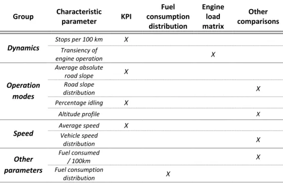
In Table 3 a summary of the parameters used in this thesis to compare simulation results to operational data is presented. The table shows the different groups that represent different parts of driving patterns. It also shows the developed comparison tools (Key Performance Indicators (KPI), Fuel Consumption, Engine Load Matrix and other parameters, which are explained in detail later) and which characteristic parameters are included within each tool.

(25)

15

Table 3. Parameters chosen for comparison and in which tool they are evaluated.

Group Characteristic parameter KPI Fuel consumption distribution Engine load matrix Other comparisons Dynamics Stops per 100 km X Transiency of engine operation X Operation modes Average absolute road slope X Road slope distribution X Percentage idling X Altitude profile X Speed Average speed X Vehicle speed distribution X Other parameters Fuel consumed / 100km X Fuel consumption distribution X

The goal of the method is that when simulating and executing the drive cycle with the same vehicle specifications as the underlying vehicle, the simulation should yield similar results for the comparable parameters of the operational data.

4.2. Comparing against operational data

To evaluate if the drive cycle yields the same output as the operational data, simulations with the CVV1 are conducted, performing the designed drive cycle. The simulation model explained in Chapter 3.2 is used, and post processing of the simulation results is made to get comparable parameters in the same format as in the operational data base.

All comparable parameters are divided into three main parts when comparing. The first comparable parameters are so called KPI-values, (Key Performance Indicators) which give the first design ideas on what general layout the cycle should have. The second comparison is the fuel consumption of the vehicle. The final comparison is to look at the engine load matrix to ensure a similar engine usage. These ways of comparing are described further below.

4.2.1. KPI

In order to make a first selection of a drive cycle that can be redesigned to better fit the operational data, an Excel table is designed. This table uses some of the characteristic parameters as input that could be attained through statistically analysing the drive cycle before simulation. By comparing many different, already existing drive cycles, and also inserting the operational data of the vehicle, a colour scheme is made to better visualize what cycles are the closest ones to the investigated operational data.

Figure 10 gives an example with generic data showing the layout of the KPI-table. Each row indicates a different drive cycle and the columns show the different characteristic parameters used. The colour scheme compares the drive cycles parameters to the operational data of the customer value vehicle. A dark green colour indicates a small

(26)

16

difference and a dark red colour indicates a large difference. The last column is an average of the for characteristic parameters relative difference to the operational data. This gives a weight factor which is the same for all parameters.

Figure 10. The KPI-table with generic data used to compare different drive cycles.

The statistical analysis of drive cycles is conducted by running a developed MATLAB script. This script analyses the KPI parameters from the data points of the drive cycle. The data points used are the speed, the road gradient and the corresponding time or distance points. The average speed is calculated for speeds above 0 km/h. When calculating the stops / 100 km, it counts the number of times the speed goes from positive to 0 km/h and uses the length of the drive cycle to convert it to a fixed length for comparison. The share of idling analyses the time spent with speeds at 0 km/h and thus neglects idling when coasting and does not separate idling with or without power take off. This was considered alright for long haulage trucks, but this methodology could be necessary to change if applied to other types of trucks which uses power take out when standing still. Some examples of vehicles were this is occurring are garbage trucks, timber trucks or mining vehicles.

4.2.2. Fuel Consumption

The next part of comparison process is the fuel consumption of the vehicle when performing the drive cycle. This measure is of high significance when designing the drive cycle due to the goal of having a similar fuel consumption between the simulated drive cycle and the operational data.

By simulating the chosen or modified drive cycle, with the truck that one aims to create a cycle for, it is possible to get a figure on the fuel consumption for that truck and drive cycle. In the operational data, the fuel consumption is given in the measure of fuel consumed per 100 km and also given as distribution of fuel consumed per velocity bin. The explained simulation model outputs how much fuel is consumed by the vehicle model when performing the drive cycle. After simulation, developed scripts are used to analyse the results and categorize the consumed fuel in the same categories as given in the operational data. In order to give a good overview on how much the distribution differed, the simulated data is plotted together with the operational data. The categories vary in ranges of 5-10 km/h per bin starting from <3 km/h and going to >105 km/h.

v_drive avrg [km/h] stops /100km [#] avrg abs(grad) [%] Idling, share of op time [%] v_drive avrg stops /100km avrg abs(grad) Idling, share of op time Average relative difference Operational data for

specific vehicle 77,0 8,0 0,6 12 0% 0% 0% 0% 0% Cycle 1 88,0 0,0 1,2 0,0 14% 100% 85% 100% 75% Cycle 2 75,0 12,0 0,8 16,0 3% 50% 21% 33% 27% Cycle 3 78,0 6,0 1,9 5,0 1% 25% 203% 58% 72% Cycle 4 56,4 40,0 2,4 21,0 27% 400% 287% 75% 197% Cycle 5 76,0 4,0 0,9 9,0 1% 50% 37% 25% 28%

(27)

17

Figure 11 shows an example of the distribution of fuel consumption when simulating a drive cycle compared to the operational data. The red bars are the simulated results and the blue bars shows the fuel consumption extracted from the operational data. The y-axis shows percentage of total fuel consumed and the x-axis shows the different speed categories.

Figure 11. The fuel consumption distribution for VECTO Regional Delivery cycle with the CVV1 truck.

As mentioned, the fuel consumed per 100 km is also checked to give a relevant number for comparing the drive cycle to the operational data. The length of the simulated drive cycle can vary and must therefore be limited in this investigation to 100 km. The distribution of consumed fuel gives extended information on where fuel is consumed. With that measure it’s possible to draw conclusions on what part of the drive cycle that the fuel is consumed, for example during constant speeds on highway or while driving with varying speeds.

4.2.3. Engine Load Matrix

Another measure used to compare the drive cycles representativeness is to generate an ELM from the simulation which is to be compared to the ELM from the operational data.

In the simulation, all parameters are logged for each time step. From this knowledge, it is possible to post process the results and yield an ELM with the same layout as the one given in the operational data. The layout and the parameters used in the design of this matrix is described in more detail in the Chapter 3.2.3 Engine Load Matrix.

After the simulation, a MATLAB script is used to generate the corresponding ELM for the simulation of the specific drive cycle. In order to better compare the ELM from simulation to the operational data, there is a sub-matrix designed to compare the two matrices in terms of percentage point. The matrix is referred to as the comparison matrix and takes the operating time percentages in the matrix from operational data minus the percentages from the simulated matrix. This yields the difference in terms of percentage points of

(28)

18

operating time in each cell. The difference is summarized in the cells on the top row and in the last column.

The way the comparison matrix is intended to be used, is to see in what cells the operation time from simulation is too large or too small compared to operational data. By calculating the engine speed for different vehicle speeds, knowing the gear ratio for different gears, the ELM can be analysed more closely. For example, when analysing drive cycles for Long Haulage trucks, the engine speed at final gear is relevant to compare in the ELM. By knowing this, it’s easier to analyse which part of the drive cycle is represented where in the ELM.

In Figure 12 on the next page, matrices yielded from operational data and simulation are shown in the first two matrices. On the bottom is the comparison matrix which shows the absolute difference between the two. The colour scheme for the comparison matrix is yellow for negative values and red for positive values.

(29)

19 Figu re 12 . An e xa m p le o f t h e co m p a ris o n m a tr ix u se d t o c o m p a re simu lat io n a n d o p er a tio n a l d a ta . 2 0 ,9 % 2 ,5 % 5 ,8 % 8 ,3 % 2 4 ,0 % 3 2 ,7 % 2 ,1 % 1 ,7 % 1 ,5 % 0 ,4 % 0 ,0 % 0 ,0 % S U M > 9 8 % 0 ,0 % 0 ,0 % 0 ,1 % 0 ,2 % 1 ,2 % 0 ,4 % 0 ,7 % 0 ,8 % 0 ,8 % 0 ,2 % 0 ,0 % 0 ,0 % 4 ,4 % 8 5 9 8 % 0 ,0 % 0 ,0 % 0 ,1 % 0 ,4 % 1 ,5 % 0 ,5 % 0 ,1 % 0 ,1 % 0 ,1 % 0 ,0 % 0 ,0 % 0 ,0 % 2 ,8 % 7 5 8 5 % 0 ,0 % 0 ,0 % 0 ,1 % 0 ,3 % 0 ,8 % 0 ,5 % 0 ,1 % 0 ,1 % 0 ,1 % 0 ,0 % 0 ,0 % 0 ,0 % 2 ,0 % 6 5 7 5 % 0 ,1 % 0 ,0 % 0 ,1 % 0 ,3 % 1 ,0 % 0 ,8 % 0 ,1 % 0 ,1 % 0 ,1 % 0 ,0 % 0 ,0 % 0 ,0 % 2 ,6 % 5 5 6 5 % 0 ,1 % 0 ,1 % 0 ,1 % 0 ,4 % 1 ,3 % 1 ,3 % 0 ,1 % 0 ,1 % 0 ,1 % 0 ,0 % 0 ,0 % 0 ,0 % 3 ,4 % 4 5 5 5 % 0 ,2 % 0 ,1 % 0 ,2 % 0 ,4 % 1 ,7 % 2 ,2 % 0 ,1 % 0 ,1 % 0 ,1 % 0 ,0 % 0 ,0 % 0 ,0 % 5 ,0 % 3 5 4 5 % 0 ,5 % 0 ,1 % 0 ,3 % 0 ,4 % 2 ,3 % 4 ,4 % 0 ,1 % 0 ,1 % 0 ,1 % 0 ,0 % 0 ,0 % 0 ,0 % 8 ,4 % 2 5 3 5 % 3 ,5 % 0 ,2 % 0 ,7 % 0 ,8 % 4 ,1 % 1 0 ,7 % 0 ,1 % 0 ,1 % 0 ,0 % 0 ,0 % 0 ,0 % 0 ,0 % 2 0 ,4 % 1 5 2 5 % 1 0 ,3 % 0 ,4 % 0 ,8 % 1 ,3 % 3 ,3 % 5 ,2 % 0 ,2 % 0 ,1 % 0 ,0 % 0 ,0 % 0 ,0 % 0 ,0 % 2 1 ,6 % 2 1 5 % 5 ,9 % 0 ,6 % 1 ,1 % 1 ,8 % 3 ,0 % 2 ,8 % 0 ,2 % 0 ,1 % 0 ,1 % 0 ,0 % 0 ,0 % 0 ,0 % 1 5 ,6 % < 2 % 0 ,2 % 0 ,9 % 2 ,1 % 1 ,9 % 3 ,9 % 3 ,8 % 0 ,5 % 0 ,2 % 0 ,1 % 0 ,1 % 0 ,0 % 0 ,0 % 1 3 ,9 % < 6 5 0 r p m 6 5 0 8 5 0 r p m 8 5 0 1 0 0 0 r p m 1 0 0 0 1 1 2 0 r p m 1 1 2 0 1 2 4 0 r p m 1 2 4 0 1 3 2 0 r p m 1 3 2 0 1 4 0 0 r p m 1 4 0 0 1 4 8 0 r p m 1 4 8 0 1 6 0 0 r p m 1 6 0 0 1 9 0 0 r p m 1 9 0 0 2 2 0 0 r p m > 2 2 0 0 r p m 9 ,2 % 4 ,0 % 1 0 ,3 % 6 ,0 % 1 7 ,8 % 4 9 ,2 % 1 ,1 % 0 ,4 % 1 ,2 % 0 ,8 % 0 ,0 % 0 ,0 % S U M > 9 8 % 0 ,1 % 0 ,6 % 0 ,7 % 0 ,6 % 1 ,7 % 0 ,7 % 0 ,5 % 0 ,3 % 0 ,7 % 0 ,7 % 0 ,0 % 0 ,0 % 6 ,6 % 8 5 9 8 % 0 ,0 % 0 ,1 % 0 ,1 % 0 ,3 % 0 ,7 % 0 ,9 % 0 ,1 % 0 ,0 % 0 ,1 % 0 ,0 % 0 ,0 % 0 ,0 % 2 ,4 % 7 5 8 5 % 0 ,0 % 0 ,1 % 0 ,2 % 0 ,3 % 0 ,0 % 1 ,0 % 0 ,2 % 0 ,0 % 0 ,1 % 0 ,1 % 0 ,0 % 0 ,0 % 2 ,0 % 6 5 7 5 % 0 ,0 % 0 ,1 % 0 ,2 % 0 ,3 % 0 ,9 % 1 ,8 % 0 ,2 % 0 ,0 % 0 ,2 % 0 ,0 % 0 ,0 % 0 ,0 % 3 ,7 % 5 5 6 5 % 0 ,0 % 0 ,3 % 0 ,0 % 0 ,2 % 2 ,3 % 3 ,8 % 0 ,0 % 0 ,0 % 0 ,0 % 0 ,0 % 0 ,0 % 0 ,0 % 6 ,8 % 4 5 5 5 % 0 ,0 % 0 ,3 % 1 ,1 % 0 ,6 % 1 ,7 % 5 ,1 % 0 ,0 % 0 ,0 % 0 ,0 % 0 ,0 % 0 ,0 % 0 ,0 % 8 ,9 % 3 5 4 5 % 0 ,0 % 0 ,6 % 2 ,5 % 0 ,8 % 1 ,5 % 5 ,7 % 0 ,0 % 0 ,0 % 0 ,0 % 0 ,0 % 0 ,0 % 0 ,0 % 1 1 ,1 % 2 5 3 5 % 0 ,0 % 0 ,6 % 2 ,1 % 0 ,4 % 1 ,3 % 6 ,1 % 0 ,1 % 0 ,0 % 0 ,0 % 0 ,0 % 0 ,0 % 0 ,0 % 1 0 ,6 % 1 5 2 5 % 8 ,8 % 0 ,4 % 0 ,8 % 0 ,8 % 2 ,3 % 6 ,7 % 0 ,0 % 0 ,0 % 0 ,0 % 0 ,0 % 0 ,0 % 0 ,0 % 1 9 ,7 % 2 1 5 % 0 ,0 % 0 ,7 % 1 ,0 % 0 ,9 % 1 ,3 % 9 ,0 % 0 ,0 % 0 ,1 % 0 ,1 % 0 ,0 % 0 ,0 % 0 ,0 % 1 3 ,1 % < 2 % 0 ,0 % 0 ,2 % 1 ,7 % 0 ,7 % 4 ,2 % 8 ,2 % 0 ,0 % 0 ,0 % 0 ,0 % 0 ,0 % 0 ,0 % 0 ,0 % 1 5 ,1 % < 6 5 0 r p m 6 5 0 8 5 0 r p m 8 5 0 1 0 0 0 r p m 1 0 0 0 1 1 2 0 r p m 1 1 2 0 1 2 4 0 r p m 1 2 4 0 1 3 2 0 r p m 1 3 2 0 1 4 0 0 r p m 1 4 0 0 1 4 8 0 r p m 1 4 8 0 1 6 0 0 r p m 1 6 0 0 1 9 0 0 r p m 1 9 0 0 2 2 0 0 r p m > 2 2 0 0 r p m -1 1 ,7 % 1 ,5 % 4 ,5 % -2 ,3 % -6 ,3 % 1 6 ,5 % -1 ,0 % -1 ,3 % -0 ,3 % 0 ,4 % 0 ,0 % 0 ,0 % S U M > 9 8 % 0 ,1 % 0 ,6 % 0 ,6 % 0 ,4 % 0 ,4 % 0 ,3 % -0 ,2 % -0 ,5 % 0 ,0 % 0 ,5 % 0 ,0 % 0 ,0 % 2 ,2 % 8 5 9 8 % 0 ,0 % 0 ,1 % 0 ,0 % -0 ,1 % -0 ,8 % 0 ,4 % 0 ,1 % -0 ,1 % 0 ,0 % 0 ,0 % 0 ,0 % 0 ,0 % -0 ,4 % 7 5 8 5 % 0 ,0 % 0 ,1 % 0 ,1 % 0 ,0 % -0 ,8 % 0 ,5 % 0 ,1 % -0 ,1 % 0 ,0 % 0 ,1 % 0 ,0 % 0 ,0 % 0 ,1 % 6 5 7 5 % -0 ,1 % 0 ,1 % 0 ,0 % 0 ,0 % 0 ,0 % 1 ,0 % 0 ,1 % 0 ,0 % 0 ,1 % 0 ,0 % 0 ,0 % 0 ,0 % 1 ,1 % 5 5 6 5 % -0 ,1 % 0 ,3 % -0 ,1 % -0 ,1 % 1 ,1 % 2 ,5 % -0 ,1 % -0 ,1 % -0 ,1 % 0 ,0 % 0 ,0 % 0 ,0 % 3 ,3 % 4 5 5 5 % -0 ,2 % 0 ,2 % 0 ,9 % 0 ,2 % 0 ,1 % 2 ,9 % -0 ,1 % -0 ,1 % 0 ,0 % 0 ,0 % 0 ,0 % 0 ,0 % 3 ,9 % 3 5 4 5 % -0 ,5 % 0 ,5 % 2 ,1 % 0 ,3 % -0 ,9 % 1 ,3 % -0 ,1 % -0 ,1 % -0 ,1 % 0 ,0 % 0 ,0 % 0 ,0 % 2 ,7 % 2 5 3 5 % -3 ,5 % 0 ,3 % 1 ,5 % -0 ,4 % -2 ,9 % -4 ,7 % 0 ,0 % -0 ,1 % 0 ,0 % 0 ,0 % 0 ,0 % 0 ,0 % -9 ,7 % 1 5 2 5 % -1 ,5 % 0 ,0 % -0 ,1 % -0 ,5 % -1 ,0 % 1 ,5 % -0 ,2 % -0 ,1 % 0 ,0 % 0 ,0 % 0 ,0 % 0 ,0 % -1 ,9 % 2 1 5 % -5 ,9 % 0 ,1 % -0 ,1 % -0 ,8 % -1 ,8 % 6 ,3 % -0 ,2 % 0 ,0 % 0 ,0 % 0 ,0 % 0 ,0 % 0 ,0 % -2 ,5 % < 2 % -0 ,2 % -0 ,7 % -0 ,4 % -1 ,3 % 0 ,3 % 4 ,4 % -0 ,5 % -0 ,2 % -0 ,1 % -0 ,1 % 0 ,0 % 0 ,0 % 1 ,2 % < 6 5 0 r p m 6 5 0 8 5 0 r p m 8 5 0 1 0 0 0 r p m 1 0 0 0 1 1 2 0 r p m 1 1 2 0 1 2 4 0 r p m 1 2 4 0 1 3 2 0 r p m 1 3 2 0 1 4 0 0 r p m 1 4 0 0 1 4 8 0 r p m 1 4 8 0 1 6 0 0 r p m 1 6 0 0 1 9 0 0 r p m 1 9 0 0 2 2 0 0 r p m > 2 2 0 0 r p m 7 2 -8 0 k p h 8 0 8 9 k p h 8 9 9 5 k p h 9 5 1 0 0 k p h O p e ra ti o n a l D a ta S im u la te d r e su lt s fr o m d ri v e c y c le D if fe re n c e : O p e ra ti o n a l d a ta S im u la ti o n @ F in a l G e a r % o f m ax im um fu el in je cte d d cte je in el fu um im ax f m % o d cte je in el fu um im ax f m % o

(30)

20

4.2.4. Other comparison measures

As an additional check if the drive cycle is representative compared to the operational data, it can be interesting to compare the vehicle speed distribution, road slope distribution and altitude profile of the drive cycle.

The vehicle speed distribution shows if the vehicle is travelling in the same speeds which is important in terms of simulating the drag forces on the vehicle more accurately. For example, the fuel consumption distribution and engine load matrix might be similar to the operational data, but the vehicle can have performed this whilst driving at lower speeds than its true operation, and the air drag is thus represented lower than it should.

The road slope distribution can in the same way show flaws in the drive cycle. The simulation might yield a satisfactory fuel consumption distribution and ELM even if it is driven on a flatter road than in operation. The simulation of braking energy and uphill driving is then to low in the simulation compared to operational data.

In order to accurately represent the full operational data in a shorter drive cycle, it’s important that the vehicle model does not perform a cycle which ends up at an altitude lower or higher than it started. This would cause the potential energy in the end of the simulation to be different than at the beginning. For the operational data, the vehicle drives so long that it is assumed that the total driving gives a difference in altitude of 0 m.

To get all these comparison tools to accurately reflect the operational data is very time consuming and depending on what the drive cycle should represent, some measures are of higher significance than others. For this thesis, the goal was to represents fuel consumption and the engine load matrix accurately.

4.3. Driving cycle design methodology

After selecting different parameters to analyse the representativeness of the cycle, a methodology on how to design the drive cycle is developed. The general idea is to choose a pre-existing drive cycle and redesign it (by parts or as a whole) to get the same output from simulation for the selected parameters as in the operational data base.

4.3.1. Choose a cycle to start with

The first step is to choose a drive cycle which is similar to the operational data in terms of the comparable characteristic parameters presented in Table 3. This drive cycle is referred to as the base drive cycle.

This is done by first assessing the KPI values from the operational data base and then inserting these in the Excel table for the KPI’s. In the table there should be data pre-inserted which holds the KPI-values for many different, already existing drive cycles. Depending on the type of truck which the drive cycle is generated for, drive cycles that are aimed for the same usage as the truck in question should have been inserted in the table. With the data inserted, it’s up to the designer to tell which drive cycle fits the best.

After choosing a base drive cycle, a simulation of it should be performed with the vehicle in question. For this thesis, the simulation is done with the Simulink model presented in Chapter 3.2. From the simulation, the designer can analyse the fuel consumption, engine load matrix and results for the other comparison measures.

(31)

21

4.3.2. Redesigning to fit fuel consumption comparison

Before changing the drive cycle to fit the distribution of fuel, which itself shows share of total fuel consumed, the fuel consumed per 100 km should be reviewed. Some parameters that influence the engine’s workload and thus the fuel consumption are acceleration levels, number of stops, speed of vehicle and road gradient [9]. These parameters can be changed by moving the speed or road gradient set points in the drive cycle. If too little fuel is used, one approach could be to increase the drive cycle’s road gradient which increases the fuel consumption.

In order to get a fuel consumption distribution which is similar to the operational data, one way of achieving this is to change the duration of driving in certain speeds. This will cause a portion of the total fuel to be used at these specific speeds. In order to achieve a consumption of fuel at lower speeds in a realistic way, stops should be included, letting the vehicle use fuel in lower speeds.

Figure 13 shows an example of how a basic drive cycle was redesigned to better fit operational data. In the drive cycle, the speeds were changed to have the same share of fuel consumption from operational data. This causes the fuel consumption to become similar to the requested consumption. The left two graphs in the figure show the base drive cycle and its corresponding fuel consumption distribution. The right two graphs show the redesigned base drive cycle and its corresponding fuel consumption. The purpose of the figures is to show the general trend of how the fuel consumption distribution changes when the speed profile is modified.

(32)

22

Figure 13. Example on how a drive cycle was changed to better fit the targeted fuel consumption distribution in blue. The left figures are the base drive cycle, the right figures

are after changing the speed points.

This way of redesigning is iterated until yielding a satisfactory result between simulated and operational fuel consumption data, that is to fit the red bars with the blue bars and to have the correct fuel consumption per 100 km.

Important to keep in mind is that when changing the speed profile of the drive cycle, the average speed of the full cycle is changed. This could cause the simulation to neglect some resistance forces which are dependent on the vehicle speed and overall energy consumption.

(33)

23

4.3.3. Redesigning to fit Engine Load Matrix

When the design of the drive cycle yields a simulated fuel consumption, similar to the operational data, the next step is to make sure that the engine operates like its true operation. This is done by comparing the simulated engine load matrix to the one from operational data.

With an accurate representation of the fuel consumption distribution, the simulated engine work should be rather similar as well, compared to the operational data. However, from experience in designing drive cycles, it was noticed that there could often be differences in how fluctuating the engine was operating in the engine load matrix. For example, the drive cycle could often yield satisfactory fuel consumption without having to operate at high and low loads but rather in a very small operating range. In order to match the engine’s work in the simulation closer to the operational data, accelerations and road gradient was changed to make the engine work more fluctuating throughout the cycle.

The engine load matrix presented and explained in Chapter 3.2.3 depends on parameters affecting the engine’s speed and load such as gear shifts, vehicle speed and road gradient.

In order to alter the engine’s use in the y-range (percentage of maximum fuel used), the engine’s load needs to be affected. A larger spread is caused by having higher accelerations as well as increasing the roads gradient. This is done by changing the speed and gradient data points of the drive cycle.

Due to the truck having a gear shift algorithm, the timing of the gear shifts and engine speed cannot easily be decided by changing the transient parts of the drive cycle. One way to alter the matrix in the x-range (engine speed) is to change the vehicles speed whilst in final gear. An accurate fuel consumption distribution should have yielded a somewhat similar engine load matrix layout in the x-axis but smaller changes to the drive cycle’s speed (1-5 km/h) could be necessary to move the engine’s operation from one engine speed column to another.

Figure 14 and Figure 15 show an example of how the ELM is changed by altering the speeds whilst in simulated operations in the final gear (speeds 77-85 km/h). The top figure,

“cycle 1” shows a generic speed and gradient profile and the lower, “cycle 2” shows the

same speed profile but with 50 % road gradient relative to the previous layout, thus changing the engine’s operation. The purpose of the figures is to show the general trend of the ELM when road gradient is modified.

(34)

24

Figure 14. Generic drive cycle with corresponding ELM.

Figure 15. Drive cycle with corresponding ELM. Same speed profile as figure 14 but with 50% of its gradient.

Another way to also modify the resulting ELM is to change parts of the gradient profile where the designer knows it will impact a certain rpm-bin. However, it’s important to keep in mind that when changing the road gradient for parts where the vehicle speeds are high, a change in road gradient will cause the vehicle to gain (or lose) altitude quicker than at lower speeds because the vehicle travels further per time unit.

Since the engine’s operation is changed when designing a good fit for the ELM, the fuel consumption, which is correlated to the engine’s work will change. This can cause the fuel consumption distribution graph to be too offset. This is part of the iterative process and can be time consuming for the designer.

Cycle 1: 100% road gradient

Cycle 2: Same speed profile 50% road gradient

(35)

25

4.3.4. Check of plausibility

After having designed a drive cycle which satisfies the designers goals for the KPIs, fuel consumption and ELM, the drive cycle should be checked for plausibility. That means to check so that the drive cycle is a reasonable representation of real driving.

A first step is to check the data points in the drive cycle and analyse its speeds and accelerations. For example, when designing a drive cycle for trucks, the cycle should not have target speeds above the vehicles intended use (80-90 km/h). A check for the acceleration levels can also be relevant to perform, in order to make sure that the drive cycle has realistic driving patterns in it, meaning that the speeds that the vehicle should perform are close to how an actual drive with the vehicle would look like.

Another measure to check when settling for a design is the final altitude relative to the starting point of the drive cycle. If the vehicle does not end up in a similar height as the starting point, then the vehicle must have put in or gained potential energy which is not favourable. Adding potential energy when performing the drive cycle will cause the fuel consumption to be incorrect when representing real driving. In order to avoid this error, the designer should check at what altitude the vehicle will end up at when using the drive cycle. An example of how to check this is shown in Figure 16 where the vehicle’s altitude is plotted over the driven distance. In this example of the drive cycle 1000 punkte [13] which is often used to test HDV, the vehicle ends up -10 m relative to the starting point. That means that after driving the drive cycle, the vehicle could use the potential energy corresponding to these 10 meters and gain kinetic energy without having to use any fuel.

Figure 16. Altitude profile for the drive cycle 1000 punkte.

Some other comparisons that can be made is to see if the drive cycle after the redesigns still has a speed and gradient distribution which is similar to the operational data. This data is available in the database and the data from the designed drive cycle can be attained by analysing the drive cycle’s speed and gradient points.