The Macroeconomic Forces Behind
Stock Market Return
Paper within Finance Master
Author: Hampus Jörnmark
Tutor: Per-Olof Bjuggren
Louise Nordström
i
Abstract
This paper deals with the forces behind stock market return in the U.S. In order to test the relationship, 10 variables are chosen and then applied to the APT model. The data is divid-ed into three periods and then a linear regression is performdivid-ed on each period. Throughout the three periods and thus through the period 1980-2011, Current Account, Money Supply and Price of Petroleum were not significant at any of the three periods at any level of sig-nificance. While the Consumer Confidence Indicator, Consumer Price Index, Federal Funds Rate, Treasury Security, Industrial Production, New Orders Index and Unemploy-ment were significant on at least one occasion.
Acknowledgements
I would like to start by thanking my two tutors, Per-Olof Bjuggren and Louise Nordström for helping me and guiding me with every aspect throughout the entire process of writing this thesis. I would also like to thank my good friend and discussant, Dan Gustafsson, who contributed by pointing out weaknesses and by suggesting some improvements.
iii
Contents
1
Introduction ... 1
1.1 Problem discussion and purpose ... 1
1.2 Research questions ... 2
1.3 Disposition ... 2
2
Background ... 2
3
Theoretical framework ... 4
3.1 Arbitrage Pricing Theory ... 4
3.2 Efficient market hypothesis (EMH) ... 5
3.2.1 Arbitrage ... 7
3.2.2 The different forms of market efficiency ... 7
3.3 Liquidity trap ... 8
4
Commonly used APT variables ... 9
4.1 S&P 500 ... 9
4.2 Independent variables ... 9
4.2.1 Consumer Price Index (CPI) ... 10
4.2.2 Consumer Confidence Indicator ... 10
4.2.3 Current Account ... 10
4.2.4 Price of Petroleum ... 11
4.2.5 Unemployment ... 11
4.2.6 Industrial production ... 11
4.2.7 Manufacturing New Orders Index ... 11
4.2.8 Federal funds rate ... 12
4.2.9 Treasury security ... 12 4.2.10 Money supply ... 12
5
Methodology ... 13
5.1 Data collection ... 13 5.2 The regression ... 146
Empirical results ... 14
6.1 Regression output 2002-2011 ... 14 6.2 Regression output 1990-1999 ... 15 6.3 Regression output 1980-1989 ... 15 6.4 Market sensitivity ... 197
Concluding remarks ... 21
8
Further studies ... 22
9
Robustness ... 23
9.1 Test for autocorrelation ... 23
9.2 Test for multicollinearity ... 23
10
List of references ... 24
11
Appendix ... 27
11.1 The IS-LM framework ... 27
11.1.1 The LM curve and monetary policy ... 28
11.1.2 The IS curve – and fiscal policy ... 29
11.2 Robustness ... 31
11.3 Regression outputs concerning market sensitivity ... 34
Regression output 1980-1984 ... 34 Regression output 1985-1989 ... 34 Regression output 1990-1994 ... 35 Regression output 1995-1999 ... 35 Regression output 2002-2006 ... 36 Regression output 2007-2011 ... 36
1 Introduction
The topic about driving forces of stock market return has been subject to much research and one can understand why so many find it interesting. The reason I chose to look at this area of the finance world is because it is so vast and complex and there is still a chance to contribute with a new perspective on the subject.
„An "efficient" market is defined as a market where there are large numbers of rational, profit maxi-mizers actively competing, with each trying to predict future market values of individual securities, and where important current information is almost freely available to all participants.‟ Eugene F. Fama 1965.
Knowing how the market will behave as a response to changes in our economic environ-ment is crucial for those who are looking to earn a return on their investenviron-ments. Chen et al (1986) argue that the forces that alter the stock price are those forces that affect discount factors, the argument is also supported by Grossman et al (1981).
Greenspan (2004) discusses how the Fed responded to the crash of the New York stock market in October 1987 by injecting the market with massive amounts of funds. Most of this effort was aimed at keeping the payment systems operational and the markets open. Due to concerns of what the aftermath would be, the policy continued into 1988.
Monetary policy and its effects on the financial system is merely one part of a vast puzzle consisting of other macroeconomic factors. These factors can be inserted to models in or-der to predict what will happen in the economy in the future and one such model is the APT model.
The CAPM uses one single risk factor; the beta coefficient, i.e. CAPM assumes that risk is only related to the market beta. In 1976, economist Stephen A. Ross introduced a new model which allowed for the use of many risk factors. The model was named the APT model, where APT is short for Arbitrage Pricing Theory. As the model was introduced, re-search was now aimed at identifying risk factors that could help explain the price move-ments of assets. In this paper I will consider 10 macroeconomic variables that I believe have an impact on the discount factors and thus also on stock prices.
1.1
Problem discussion and purpose
Several previous studies have been conducted where statistical proof has been found to support the theory that macroeconomic factors affect the stock market, some of which will be mentioned in the background section of the paper. There has also been research to sup-port that some macroeconomic factors have little or no effect at all on our stock markets, e.g. Chen et al (1986) find that the price of oil has no influence over stock market return. To test whether macro variables affect the stock market, I will use the APT model, devel-oped by Ross in 1976, since this model allows for the use of several variables when predict-ing expected returns.
Technology has made huge progress since the introduction of the stock market and it is still evolving. But how do our financial markets respond to information compared to be-fore? Perhaps it responds faster and to a larger extent, as the flow of information is close to immediate and perhaps even unlimited.
The main purpose of the paper is to investigate and observe what macroeconomic factors drive stock market return in the US and thus also which variables that have the largest ex-planatory power, secondly to observe if the market is becoming more responsive to chang-es. In order to fulfill the purpose I will use Ross‟s APT model where I will include the mac-roeconomic factors I believe influence the stock market return. This brings me to the two research questions below.
1.2 Research questions
What macroeconomic variables drive stock market return?
Is the market more responsive to changes today than it was before?
1.3
Disposition
The next section of the thesis starts off with a brief background containing previous re-search. Section three deals with the underlying theory needed in order to grasp the bigger picture of the thesis. Section four is the method chapter where I tell you about how I in-tend to put the theory into work and the last section contains the empirical results and the conclusion.
2 Background
The first stock exchange to ever see the light of day was the Philadelphia Stock exchange in the U.S and the year was 1790, (bloomberg.com). But it wasn‟t until 1971 that the first elec-tronic stock market opened up for business, namely the NASDAQ stock exchange, (nasdaqomx.com). Essentially what this means is that before 1971 the system was only a bulletin board that did not connect the sellers with the buyers. Today, buyers and sellers worldwide are able to communicate to each other and retrieve price information and quotes in real time. I.e. information which is crucial to the commodity that they want to sell or buy; therefore as trading volumes become large, time is of the essence.
„The most familiar interpretation for the large and unpredictable swings that characterize common stock price indices is that price changes represent the efficient discounting of new information‟ Grossman et al (1981)
Apart from making this statement, the authors investigate whether the variability of stock prices can be explained by discount factors. The authors find that the present value of real
dividends using the stock price in 1979 as a terminal value and the real S&P Composite Stock Price Average are two leading indicators of future economic activity.
Chen et al (1986) discuss the existence of „state variables‟ and that the co-movement of as-set prices would imply an impact from other economic variables. The authors argue that the price of a stock can be written as a function of the future dividends that we expect the stock to earn, divided by a discount factor. Thus the forces that we would assume to affect the price of a stock are those forces that change the discount factors. The conclusions drawn by the authors are that the variables that are most significant in explaining stock re-turn are industrial production, changes in the risk premium, unexpected shifts in the yield curve and to some extent unanticipated inflation and changes in expected inflation.
(Choi & Jen 1991) investigate the relation between expected stock returns and short-term interest rates. Specifically, the authors examine to what extent common stock returns are related to the risk associated with uncertain movements in short-term interest rates. What they found out was that small firms were more responsive to changes in the interest rate than large firms and also that the short-term interest factor, also known as the federal fund premium has a large explanatory power over the expected return of stock listed on the NYSE.
Jensen et al (1996) investigate as to whether monetary policy effects can explain expected return; they conclude that expansionary monetary policy can be used to predict future re-turn on the stock market. Another conclusion drawn by the authors is that the term spread no longer is significant when trying to forecast stock returns. As a final remark, the authors summarize by stating that they found support that Fama & French‟s (1989) conclusions are accurate, that it is rational to believe that prediction of expected stock and bond return is possible and that the return to some extent is related to monetary and business conditions. In the paper by Conover et al (1998) the authors find that regions with a high expansion-ary monetexpansion-ary policy exhibit higher return on the stock market, than those regions which have adopted a restrictive monetary policy and that this return not necessarily is associated with a higher risk. Of the 16 countries that were studied, 14 of the countries show stock market returns which are linked to the monetary policy implemented by the country. Mann et al (2004) also investigate the sensitivity of stock returns to monetary policy but with respect to two different groups which are based on the federal funds rate and the U.S. discount rate, in total the paper examines five different monetary policy variables taken from these two groups. The chosen variables are two binary variables from the first group, the spread of the federal funds rate to 10-year treasury securities, the change in the federal funds rate and the average federal funds rate. They then use ordinary least squares (OLS) and use the S&P500 as the dependent variable and the chosen monetary policy factors as the independent variables. Their findings indicate that even though the binary variables are significant, their explanatory power over stock market return is questionable.
3
Theoretical framework
This chapter deals with some of the underlying theory of efficient market hypothesis, the liquidity trap, the arbitrage pricing theory along with an explanation of the variables I have chosen to include in my model.
3.1 Arbitrage Pricing Theory
The arbitrage pricing theory or the APT model was developed by Stephen A. Ross in 1976 and is an alternative approach to the CAPM. Both CAPM and the APT illustrate the rela-tionship between risk and return, although CAPM assumes that return is related only to the market beta, the APT allows for the use of more variables when predicting the expected re-turn. The APT also differentiates between systematic and unsystematic risk but allows us to add variables to our model until the unsystematic risk has vanished. That is, factors which influence the discount rate. (Ross et al 2010)
“An asset pricing model is a success if it improves our understanding of security market returns. By this standard, the APT is a success.” Connor & Korajczyk (1993)
Connor & Korajczyk acknowledge that the APT does have weaknesses, but when the APT is compared to other models created for the same purpose, it has performed well. They al-so point out that the advantage of using such a multifactor model is that such models offer a better approximation of the random discount factors. Despite its simplicity, the structure behind the APT model is used today by companies such as MSCI (msci.com) and North-field (northNorth-field.com).
The relationship between risk and return can be modeled as follows;
(3.1)
Where represents the risk free rate, is the expected excess return, and , which is the beta on the market, with representing the variance of the market portfolio and being the covariance of asset i with the market portfolio. A high-er risk is associated with a highhigh-er return, because investors require a highhigh-er return for tak-ing on additional risk.
Since the APT model is a multi-factor model and allows for the use of multiple variables, we can illustrate the relationship with equation 3.3
where is a random term and is equal to the actual value – the expected value of the variable. Assume that the expected inflation be equal to and let actual inflation be de-noted as . Now assume that the expected inflation to prevail at is 2,8% but when we arrive at the actual inflation is 3% instead, we then say that = 0,2%. What variable to include in the APT model is up to the user and should simply be chosen with respect to what is being tested. A variable that provides little or no explanatory power to the model can still be omitted in the end.
Let us now elaborate and continue by saying that the return can be divided into two parts; the expected and the unexpected part. The expected part consists of what people expect or predict by using the information set that is available to them right now. The unexpected part stems from information that will be revealed within the time frame of the prediction, next month‟s share price for instance. In this case, the unexpected part comes from infor-mation that will be available within the month. We can model the relationship with equa-tion 3.4
(3.3) R =R + U where R is the actual return,R is the expected return and U is the unexpected part of the return, which is also referred to as the risk of the investment. (Ross et al 2010) U can also be divided into two parts, systematic risk and unsystematic risk, which we then denote as m and ε for systematic and unsystematic risk respectively. The systematic risk is related to events that will affect a large number of firms on the market, such as an earthquake, while unsystematic risk refers to evens that are specific for a firm, such as when a new project is completed or a chairman dies or resigns.
The systematic risk is denoted as β (beta) in equation 3.5 and it tells us how much the de-pendent variable fluctuates as a response to an exogenous impact from a systematic risk variable, i.e. a beta of 2 means that a 1 percent change of a systematic risk variable will cause a 2 percent change of the dependent variable. I can now model the relationship with equation 3.5, which contains K number of variables. (Ross et al 2010)
(3.4) R
3.2 Efficient market hypothesis (EMH)
An efficient market can be defined as a market where share prices fully reflect all the in-formation available to investors Fama (1970). Further, the effect is immediate, meaning that when information is released the market reacts immediately and prices adjust accord-ingly. (Ross et al 2010) The macro variables I have chosen to work with can be viewed as information that is constantly being revealed to the public and thereby also incorporated in to share prices if the market is rational. This section is therefore aimed at explaining the basic theory in the EMH.
The market’s response to new information1
Figure 3.1
Figure 1 illustrates how information is incorporated in three different market settings. The solid line shows that in an efficient market, information is incorporated in the share price immediately as new information is revealed. The dots represent the response in a slow market setting, where the adjustment process can take up to 30 days in this picture. The dashed line illustrates a market that overreacts as new information is revealed, so instead the share price rises too much before reaching its “intrinsic” value, so to speak. (Ross et al 2010)
Shleifer (2000) argues that there are three different conditions, where any one of them will cause market efficiency. These three conditions are rationality, independent deviations from rationality and arbitrage. In order to fulfill the purpose of this paper, only arbitrage is relevant.
1 The theory and imagery found in figure 1 was obtained from Ross et al „Corporate finance‟ 2010, however created by the author for this paper.
3.2.1 Arbitrage
Now imagine a market where there are two types of investors on the market: The irrational amateur and the rational professional. The amateurs will act on the market, driven by their emotions. This irrational behavior will cause share prices to rise or fall from the market prices. Now, let‟s add the rational professionals to the picture. They do business based on information which they acquire through careful investigations of the companies. They buy and sell at a low and at a high price respectively. They would also be willing to spend a large portion of their wealth at a security, since they know that it is mispriced. Arbitrage gener-ates a profit when securities are bought and sold, but even if these professional arbitrageurs dominate the amateurs on this market, the particular market would still be an efficient mar-ket.
3.2.2 The different forms of market efficiency
Weak form
According to Fama (1970) a market is said to be weak-efficient if current share prices reflect the information contained in previous share prices. The weak-form efficiency can be described with the following equation.
(3.5)
Where is the price today, is the last observed price, is expected return and is the random component. If an investor is not able to earn an excess return simply by looking at past return, the market is said to be weak-efficient. This is the weakest form of efficiency a market can reach.
Semi-strong
In a semi-strong market, current share prices reflect all publicly available information Fama (1970). If any market is to reach this level of efficiency, an investor will not be able to make a profit simply by using the information obtained from a public an-nouncement.
Strong form
If the market is to reach the strong form efficiency, current share prices need to con-tain all information available, both public and private. (1970). Even if any investor is able to obtain information before the public, he is not able to evaluate the value of the information and thus he can‟t earn an abnormal return.
The main purpose of the thesis is to investigate what macroeconomic forces that drive stock market return. Information about macroeconomic conditions is available online and
in various publications. Basically, we can look at it as information which is constantly being revealed to the public. Further, the adjustment process is immediate and therefore the data will not be lagged Ross et al (2010).
3.3 Liquidity trap
A liquidity trap is a phenomenon when monetary policy has little or no effect in stimulating the economy because nominal interest rates are close to zero, thus making people indiffer-ent between holding money or bonds. If people view bonds as a substitute for money, this means that the supply of money does not matter. Krugman et al (1998) I.e. when the inter-est approaches zero needless to say, monetary policy cannot lower the interinter-est rates further. Though this occurrence appears regularly in textbooks as an example to provide the reader with an illustration, this actually happened in Japan in the end of 1990, where interest rates went from a few percent all the way down to the zero line! Dornbusch et al 2008.
Japan experienced the liquidity trap but that could never happen in Europe or USA could it? On his blog, Paul Krugman argues that most of the civilized world has experienced or are currently caught a liquidity trap, nytimes.com (2012). The federal funds rate is the inter-est rate which is targeted by monetary policy. Figure 2 displays the federal funds rate for the period 1990-2011, ranging from 8.2% in January 1990 to 0.08% in the late 2011.
Figure 2 0 1 2 3 4 5 6 7 8 9 19 90-01 19 90-11 19 91-09 19 92-07 19 93-05 19 94-03 19 95-01 19 95-11 19 96-09 19 97-07 19 98-05 19 99 -03 20 00-01 20 00-11 20 01-09 20 02-07 20 03-05 20 04-03 20 05-01 20 05-11 20 06-09 20 07-07 20 08-05 20 09-03 20 10-01 20 10-11 20 11 -09 Fed. Fun ds r at e
4
Commonly used APT variables
4.1 S&P 500
The dependent variable and thus also representing the market portfolio is Standard & Poor‟s 500 Index. The reason I chose this particular index is that it contains 500 stocks where the majority are companies that are American. This suits the purpose of this paper, since I am using data from the U.S. thus making the S&P 500 a good substitute for the market portfolio. From a statistical point of view, this particular index is preferable since it includes both value and growth stocks, with growth stocks being the more volatile of the two. In addition, I will consider the adjusted close price to account for events such as splits and new emissions.
4.2 Independent variables
The CPI and the Unemployment rate are two important and common macroeconomic fac-tors that we frequently hear about on the news or in textbooks, where their importance frequently is stressed.
The Consumer Confidence Indicator is interesting from a household‟s perspective and not just on a business or country level. I.e. I wanted to include something to represent the av-erage American household.
The Current Account and Money Supply were chosen due to their connection to the IS-LM framework and thus also their ability to affect economic activity. I wanted to include the Federal Funds Rate & Treasury Security since not all previous research point in the same direction. Choi & Jen (1991) find strong evidence that the Federal Funds Rate has explanatory power over stock return listed on the NYSE, while Mann et al (2004) find weak support that interest rates based on the Federal Funds Rate and the discount factor are significant over the tested time period. Further, Industrial Production is a worthy can-didate for my regression due to its capability of predicting short term economic activity. The New Orders Index is nominated due to its association to the stock market (Lundin et al 2011). Chen et al (1986) found little or no evidence that the price of crude oil had an ef-fect on the return on the stock market, but rather to include the very same variable, I chose to include it with a slight modification. The variable now displays the price of domestically produced petroleum in the U.S, rather than the crude oil price.
I have chosen to look at how much each variable increased from the previous period, (month in this case) measured in percent. Since the S&P index can be converted in to the same manner, I can apply the data to my model when I start my empirical work.
4.2.1 Consumer Price Index (CPI)
The consumer price index, or the CPI, measures the price change in per cent on a stand-ardized basket of goods with a certain year as the base year. The base year is then denoted as 100 and if we were to experience a 5% increase in the overall price level over the coming year, the next year‟s CPI would take on the value of 105. CPI thus provides us with a way of measuring the change in the purchasing power of the currency that we are dealing with, in this case the USD.
The CPI has sometimes been accused of overstating the level of inflation, however it re-mains the most commonly used aggregate price statistic in the US, Bryan and Cecchetti (1993) and that is the reason I use it to represent my inflation variable.
4.2.2 Consumer Confidence Indicator
The consumer confidence indicator (CCI) is part of the OECD‟s main economic indicators (MEI). After the primary data have been collected, it goes through a standardization pro-cess in order to make comparisons between countries possible. The indicator uses 100 as the base and captures patterns of the consumption by households and thus not by the in-dustry. (OECD 2006)
The CCI is based on a survey with questions regarding the financial situation, general eco-nomic situation, employment situation and savings situation of the household over the next 12 months. The indicator is then stated in the form of the positive versus negative results. Each question has 5 possible answers where double weight is assigned if the person an-swers with any of the extremes and zero weight is given for the neutral answer.
4.2.3 Current Account
The current account shows the relationship between exports and imports. The United States has had a negative current account since the 1990‟s which means that the country‟s imports exceed its exports. The current account is part of the balance of payments and fits into the below equation.
(4.1)
Where NX is the difference between imports and exports, also known as net exports and
Since NX is part of the IS curve, an increase in exports causes the IS curve to shift to the right, at a point where both output and the interest rate has increased. Refer to the IS-LM section in the appendix for further illustration.
The data for the current account was stated on a quarterly basis, it was transformed into a monthly manner using cubic spline interpolation and matlab. This type of data
transfor-mation implies that each data point is dependent upon the previous one. This phenomenon is known as autocorrelation and in the robustness section I will test if there is autocorrela-tion present. Since there was no published data for the last quarter of 2011, I used expo-nential smoothing to generate a prediction for the last quarter.
4.2.4 Price of Petroleum
This variable displays the price of petroleum. Since Chen et al (1986) proved that the crude price of oil had no explanatory power over stock market return, this variable has been slightly modified to display the price of domestically produced petroleum in the U.S.
4.2.5 Unemployment
The type of unemployment that this variable is measuring is called Harmonised Rate of Unemployment (HUR), the standard has been adopted by 29 countries, including the US. HUR makes international comparison easier and this standardization is one reason that I chose to use it. (OECD.org, news release)
The measure is based on definitions of the 13th Conference of Labour Statisticians, which is also referred to as the ILO guidelines. HUR shows, in accordance with these guidelines, the number of unemployed, measured as a percentage of the work force, with the work force defined as civilian employees, the self-employed, unpaid family workers and the un-employed. However, according to ILO, people only counts as unemployed if they are of working age and in a specified period are without work, available for and actively seeking work. (OECD.org)
4.2.6 Industrial production
Industrial production measures the output of the economy‟s industrial sector. The industri-al sector contains manufacturing, mining and utilities. Chen et industri-al (1986) found evidence that it possesses explanatory power over the independent variable. Rather than substituting this variable for something that might not do much good for our model, I chose to include it since it is a good measure of short term economic activity. It is also included in the OECD‟s list of main economic indicators.
4.2.7 Manufacturing New Orders Index
Established 1915, the Institute for Supply Management (ISM) was the first supply man-agement institute in the world. (ism.ws) The ISM consists of two parts, one is focused on services and the other is focused on the manufacturing part and each research looks at ap-proximately 400 corporations. The Manufacturing New Orders Index is one of the 10 in-dexes that are covered by the ISM and it is considered a good predictor of the stock
mar-ket. The New Orders Index measures the level of new orders made by customers consist-ing of either manufactures or non-manufactures, this is why it is considered a good indica-tor of economic activity, especially when put in relation to stock market activity. (Lundin et al 2011).
4.2.8 Federal funds rate
The interest rate, both long term and short term, can be viewed as the time value of mon-ey, the opportunity cost of holding money and the price of borrowing money. Lower inter-est rates thereby typically mean reduced cost of borrowing funds, lower opportunity cost of holding funds and lower capital costs. Further, this implies a higher investment spending by firms.
The federal funds rate is used as the short term interest rate and it is an overnight or a one-day rate, where banks and other financial institutions can borrow funds from the Federal Reserve. It is considered an important interest rate in the US capital market because it is the best estimate to an instantaneous spot rate (Spindt & Hoffmeister 1988) but also be-cause it plays a key role when monetary policy is implemented (federalreserve.org), refer to the appendix for the basic theory in monetary policy and how the interest rate can be al-tered.
4.2.9 Treasury security
The long term interest rate is represented by the 10-year treasury security. The relationship between risk and return implies that the long term interest rate is higher than the short term interest rate, due to the increased risk associated with a longer time period that any particular investor is forced to hold the security. During a 10 year period, there are more uncertainties that cannot be accounted for, so investors who purchased a security with a longer maturity require a higher return to account for these uncertainties.
4.2.10 Money supply
The amount of money in the U.S market is regulated by the Federal Reserve, larger amounts of money in an economy typically means a higher economic activity and higher prices. Policy makers need to be aware of such tradeoffs like the one associated between inflation and money supply in the economy, when for instance monetary policy is under-taken.
The supply of money is measured in nominal terms and there are several ways to measure money supply in the economy. The type of money supply I have chosen to work with is M2. The different forms are M0, M1 and M2 with M0 being the most liquid and M2 the least liquid. Until March 23 2006, there was a fourth category, M3. However, after conclud-ing that M3 did not contribute with anythconclud-ing that M2 didn‟t already cover, the Federal
Re-serve terminated the publication of the M3 category. (federalreRe-serve.gov) Some of the types accounted for by M2 are all physical currency such as bills and notes, bank reserves, most savings accounts, money market accounts and the amount in demand accounts.
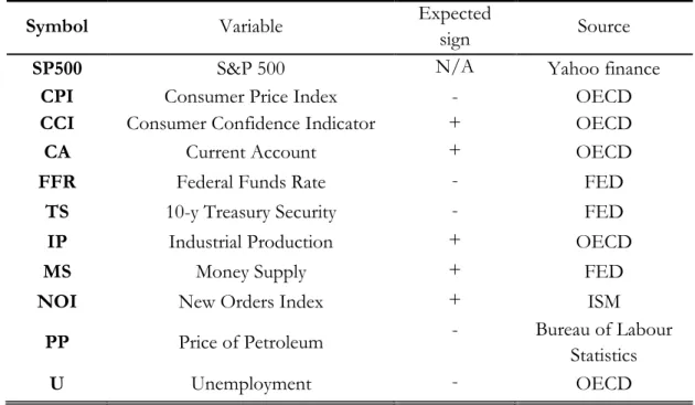
Table 4.1 Variable summary
Symbol Variable Expected
sign Source
SP500 S&P 500 N/A Yahoo finance
CPI Consumer Price Index - OECD
CCI Consumer Confidence Indicator + OECD
CA Current Account + OECD
FFR Federal Funds Rate - FED
TS 10-y Treasury Security - FED
IP Industrial Production + OECD
MS Money Supply + FED
NOI New Orders Index + ISM
PP Price of Petroleum - Bureau of Labour
Statistics
U Unemployment - OECD
5 Methodology
5.1
Data collection
Data for S&P 500 was collected from yahoo finance. The federal funds rate, treasury secu-rity and money supply data was obtained from the Federal Reserve‟s homepage. Data re-garding consumer confidence indicator, current account, industrial production and unem-ployment was collected from the OECD statistics homepage. Data for petroleum price was gathered from the Bureau of Labour statistics and the last source for my data collection was the Institute for Supply Management, where I collected data for the New Orders In-dex. The time frame for all my data ranges from the 1980‟s until 2012 and I have chosen to look at monthly data. Some of my data is in a quarterly form and all data that was not stat-ed on a monthly basis have been convertstat-ed to do so and now show the percent increase from the previous month.
5.2
The regression
In order to calculate the betas, I will run a regression on each of the independent variables on the dependent variable. The data will not be lagged, although it will be divided into three periods, in order to answer my question as to whether the market is becoming more sensitive now than it was before.
6
Empirical results
This section contains all the empirical work and it starts off with 3 regressions, each con-taining monthly data for 10 years. These three regressions are run in order to answer my first research question. Section 5.4 follows and deals with my second research question as to whether the market is becoming more sensitive.
6.1 Regression output 2002-2011 SP500 Coef. Std. Err. t P CCI*** 3.376659 .9113557 3.71 0.000 CPI 1.478741 1.063395 1.39 0.167 CA .1509101 .1207763 1.25 0.214 FFR -.0394054 .0306109 -1.29 0.201 TS .0557119 .0635571 0.88 0.383 MS .6462536 .675374 0.96 0.341 IP -.3021254 .5486372 -0.55 0.583 NOI** .1284642 .0566665 2.27 0.025 PP 1.538566 4.262721 0.36 0.719 U*** -.453084 .1631029 -2.78 0.006 R-squared 0.2776 F-value 4.19 No. of obs. 120
*** Significant at the 1% level. ** Significant at the 5% level. CPI (Consumer Price Index), CCI (Consumer Confidence Indicator), CA (Current Account), FFR (Federal Funds Rate), TS (Government Bond), MS (Money Supply), IP (Industrial Production), NOI (New Orders Index), PP (Price of Petroleum), U (Unem-ployment)
6.2 Regression output 1990-1999 SP500 Coef. Std. Err. t P CCI*** 2.411168 .8366272 2.88 0.005 CPI*** -5.610396 1.905072 -2.94 0.004 CA -.0033817 .0092851 -0.36 0.716 FFR -.18005 .0926294 -1.94 0.055 TS -.1969072 .0997096 -1.97 0.051 MS -.2508284 .6301543 -0.40 0.691 IP** -1.598725 .649965 -2.46 0.015 NOI -.054671 .0554561 -0.99 0.326 PP .0454373 .0336716 1.35 0.180 U -.0359946 .1369004 -0.26 0.793 R-squared 0.2691 F-value 4.01 No. of obs. 120
*** Significant at the 1% level. ** Significant at the 5% level. CPI (Consumer Price Index), CCI (Consumer Confidence Indicator), CA (Current Account), FFR (Federal Funds Rate), TS (Treasury Security), MS (Money Supply), IP (Industrial Production), NOI (New Orders Index), PP (Price of Petroleum), U (Unemployment)
6.3 Regression output 1980-1989 SP500 Coef. Std. Err. t P CCI*** 3.882895 1.15049 3.37 0.001 CPI -1.163086 1.444027 -0.81 0.422 CA -.0006844 .005718 -0.12 0.905 FFR .0306871 .0663049 0.46 0.644 TS** -.2884662 .1273263 -2.27 0.025 IP -1.135933 .7001246 -1.62 0.108 NOI .0323433 .0533467 0.61 0.546 MS -.2543619 .7822346 -0.33 0.746 PP .1263499 .0793032 1.59 0.114 U -.0087233 .1798442 -0.05 0.961 R-squared 0.2076 F-value 2.86 No. of obs. 120
*** Significant at the 1% level. ** Significant at the 5% level. CPI (Consumer Price Index), CCI (Consumer Confidence Indicator), CA (Current Account), FFR (Federal Funds Rate), TS (Treasury Security), MS (Money Supply), IP (Industrial Production), NOI (New Orders Index), PP (Price of Petroleum), U (Unemployment)
The Consumer Confidence Index (CCI) measures how confident households are regard-ing their future economic situation and this is why we see such a strong relationship be-tween it and the dependent variable.
The variable was significant at the 1% level of testing at all three 10-year periods. If house-holds are experiencing financial problems, they would want to choose to save at a lower risk than the stock market can offer.
Further, the coefficient of the CCI is highest for the period 1980-1989, i.e. the stock mar-ket and the CCI correlated more during this period than for later periods. Since the CCI represents the financial confidence of consumers who are triggering part of the fluctua-tions, the S&P 500 is thereby most likely subject to the mood changes of consumers. It is also possible that the CCI is affecting the discount rate, which is thereby causing stock prices to fluctuate. If consumers are confident about the future, their actions will also be incorporated in to the market assuming that the market is indeed rational.
The New Orders Index (NOI) was also expected to have an effect on the stock market due to the association between it and the stock market. (Lundin et al) It was proved signifi-cant for the period 2002-2011 at the 5% level of significance.
A higher (lower) level orders received by firms indicate that they will experience higher (lower) revenues, but also profits if the particular firm is benefiting from increasing returns to scale. A higher profit typically means that any particular firm can pay their shareholders a higher dividend, which is likely to result in a higher share price since investors‟ confidence in the company‟s performance thereby increase.
The change in Unemployment shows a strong relationship towards the change in S&P 500 for the period 2002-2011. Relating back to the stock market crash of 1929 when un-employment was very high, the impending result was a collapse of the financial system. Although we might not ever again experience such an extreme case, we are likely to be able to observe a common movement between the two, the graph below allows us to study the relationship.
A higher unemployment typically means a lower level of consumption, which partly helps explain why we can see this relationship.
Changes in unemployment and the S&P 500
Figure 6.1 Figure 3 shows the percent change in unemployment and the S&P 500 from the previous period. The arrows show some examples of peaks where we can see an opposite peak at the other side of the zero line. Throughout the time line a clear pattern can be observed be-tween the two variables. When unemployment is high, the stock market tends to move in the opposite direction. However, since we were able to see such a strong relationship be-tween unemployment and the dependent variable.
The coefficient for unemployment ranges from -0.008 to -0.450 for the periods 1980-1989 and 2002-2011 respectively, this implies a large change in the beta coefficient for the model and further suggests that the S&P500 is more receptive to changes in unemployment in 2011 than it was back in 1989.
-25,00000 -20,00000 -15,00000 -10,00000 -5,00000 0,00000 5,00000 10,00000 15,00000 1 6 11 16 21 26 31 36 41 46 51 56 61 66 71 76 81 86 91 96 10 1 10 6 11 1 11 6 12 1 SP500 U
Level of unemployment 1980-2011
Figure 6.2
Figure 4 shows the actual level of unemployment from 1980 to 2011. There‟s no actual pat-tern here that would clarify why the stock market might be becoming more sensitive to changes in unemployment as unemployment seems to actually have decreased for this time frame.
It is somewhat peculiar why the Consumer Price Index was only significant for one peri-od, 1990-1999. The inflation perceived by consumers (CPI) was expected to have an influ-ence on the stock price due to the inverse relationship associated between changes in price and consumption behavior. Economic theory tells us that a higher (lower) price typically means that consumption decreases (increases), ceteris paribus. If a larger portion of an in-dividual‟s wealth is spent on food, rent, bills, clothes etc. due to an increase in the overall price level, we are expecting that individuals are less likely to invest money on the stock market.
The level of money circulating in the economy can be thought of as being altered by the Fed, as mentioned in the appendix. The money supply was not found significant at any lev-el of significance in any of the three periods. These finding are in line with the conclusions drawn by Mann et al (2004), that the explanatory power of monetary policy over stock market return is questionable. Even though I mentioned how the use of monetary policy helped the financial markets back up their feet after the great depression. It is possible that Krugman was right when he claimed the most of the modern world is currently in a liquidi-ty trap and thereby rendering monetary policy useless. My results do indeed point me
to-0,00 2,00 4,00 6,00 8,00 10,00 12,00 Jan -198 0 May -… Se p -19 82 Jan -198 4 Ma y-… Se p -19 86 Jan -198 8 Ma y-… Se p -19 90 Jan -199 2 Ma y-… Se p -19 94 Jan -199 6 Ma y-… Se p -19 98 Jan -200 0 Ma y-… Se p -20 02 Jan -200 4 Ma y-… Se p -20 06 Jan -200 8 Ma y-… Se p -20 10 Series1
wards believing the same thing, however further research would be necessary in order for a valid conclusion to be made.
Just like money supply, Current Account also affects the price level, output and interest rates. However current account was expected to have an impact on the dependent variable due to its ability to alter interest rates, which in turn affects the discount factor and thereby also the stock price.
(Choi & Jen 1991) found evidence that the federal funds rate had a large explanatory power over stock listed on the NYSE. The Federal Funds Rate was not significant in any period at any level of significance. The Treasury Security was proven significant at the 5% level of significance for the period 1980-1989.
Although it was not significant in all my regressions, Industrial Production was proved significant at the 5% level of significance for the period 1990-1999. The same conclusion was made by Chen et al (1986).
Throughout the three periods, the Current Account, Federal Funds Rate, Money
Sup-ply and Price of Petroleum were not significant in any of the periods at any level of
test-ing. One aspect that is interesting with this finding is that current account, federal funds rate and money supply all play a key role in the IS-LM framework. I.e. out of the three var-iables that relate to the IS-LM framework, none are significant at any level of testing. The IS-LM framework thereby has no effect on stock prices for the tested periods.
Thus, for the current account, money supply and price of petroleum we cannot reject H0.
The Consumer Price Index, Consumer Confidence Indicator, Treasury Security,
In-dustrial Production, New Orders Index and Unemployment were significant on at
least one occasion and thus we reject H0 for these variables. As an investor variables such as these are thereby worth to watch closely, since they can provide information which is crucial in order to predict future economic activity.
6.4 Market sensitivity
The following section deals with my second research question as to whether the market is becoming more sensitive.
Table 6.1 Market sensitivity
*** Significant at the 1% level. ** Significant at the 5% level. *Significant at the 10% level. CPI (Consumer Price Index), CCI (Consumer Confidence Indicator), CA (Current Account), FFR (Federal Funds Rate), TS (Government Bond), MS (Money Supply), IP (Industrial Production), NOI (New Orders Index), PP (Price of Petroleum), U (Unemployment)
These are all the beta coefficients for 1980-2011. The regression outputs can be viewed in the appendix. There is no clear pattern, that would make me believe that the market is be-coming more sensitive or less sensitive either for that matter, however some of the coeffi-cients are subject to large changes, the CCI, CPI and PP for instance.
The optimal condition here would be that many variables were significant at several occa-sions, to allow me to be able to make a decent conclusion regarding what direction market sensitivity is heading. However since this is not the case, I will only conclude that the mar-ket betas are changing over time and that this change is very different from variable to vari-able. How this change is determined would require further studies.
Although the betas did not provide me with sufficient information, one interesting aspect is brought to light if we look at the r-squared for the three periods.
The r-squared is at its highest for the period 2002-2011 and the lowest for the period 1980-1989. There are of course more variables apart from the ones I have chosen, that explain stock market return, but with respect to my chosen variables it seems as if the market is re-sponding more today than it did in 1980. Although when looking at the r-squared from the 5-year regressions, the period with the highest r-squared was 1990-1994. In order to deter-mine the cause of this shift in sensitivity, more research would be needed.
If we consider the speed at which technology is evolving and the tools that people have at their disposal today, the idea that our markets respond differently seems reasonable.
Period CA CCI CPI FFR TS IP MS NOI PP U
1980-1984 0,001 2,384* -1,254 -0,028 -0,230 0,780 1,698 0,020 0,252 0,399* 1985-1989 0,011 9,691*** -2,122 0,021 -0,230 -4,019** -1,293 0,101 0,150 -0,305 1990-1994 -0,002 1,285 -5,010** -0,163 -0,167 -0,125 -2,196*** -0,045 -0,031 0,138 1995-1999 -0,020 4,665* -2,892 -0,552** -0,148 3,072*** - -0,058 -0,087 0,052 -0,006 2002-2006 0,141 3,935*** -0,147 0,055 0,256*** -1,507* 0,001 -0,044 -7,280 -0,137 2007-2011 0,288 2,592 1,089 -0,049 -0,023 -0,272 0,776 0,200** 5,186 -0,474*
7
Concluding remarks
This paper has dealt with 10 macroeconomic variables, where the purpose to fulfill was to see which variables that affect the stock market return. I performed three regressions with monthly data where each regression spanned over 10 years, the data ranged from 1980 to 2011. The regression was a linear type, where the APT model was used as a starting point. I also wanted to test if the market is becoming more sensitive. I therefore divided the data into six different 5-year segments, hoping that I would be able to see a clear pattern in the betas. No information obtained from the betas of these regressions would cause me to be-lieve that the market is becoming more or less sensitive as time passes. However for the three regressions, the r-squared was the highest for the period 2002-2011 and the lowest for the period 1980-1989. This finding made me believe that the market responds different-ly to information in different time periods. The most significant factor found to explain the return for the period 2002-2011 was the Consumer Confidence Indicator. The variable that proved most significant in the period 1990-1999 was CPI. For the period 1980-1989 the Consumer Confidence Indicator proved to be the most significant once more.
Throughout the three periods and thus through the period 1980-2011, Current Account, Money Supply and Price of Petroleum were not significant at any of the three periods at any level of significance. While the Consumer Confidence Indicator, Consumer Price In-dex, Federal Funds Rate, Treasury Security, Industrial Production, New Orders Index and Unemployment were significant on at least one occasion. The issue dealt with has been subject to much attention and some of the variables have been used before.
Although changes to the macroeconomic variables might not cause the markets to crash like in 1929, one can still understand why small changes may result in large fluctuations in the stock markets when peoples‟ expectations also are added to the equation.
My conclusion is that the extent to which the stock market is responding is changing over time and although some factors definitely seem to have a larger effect than others, the re-turn on the stock market is responding when changes occur in the economic environment. One can easily understand this reaction, as the economy or the macro economy if you will, serves as a foundation on which our financial markets reside.
8
Further studies
As mentioned in the empirical section of the thesis, the lack of explanatory power by the money supply variable could indicate that the U.S has been subject to a liquidity trap for some time. And as also mentioned, Krugman argues that most of the modern world is cur-rently in a liquidity trap. This does, in my opinion call for further studies to also investigate how severe the situation is and in order to find out what the consequences could be. The second subject that I feel requires further attention is what causes market sensitivity. Since my results did not allow me to make valid conclusions, a new study would be aimed at finding several variables which are significant throughout many periods and thereafter trying to conclude what causes this change and to what extent.
9
Robustness
The residuals don‟t appear to exhibit any patterns that might indicate that there is a prob-lem present. However, I will first run a few tests to investigate whether my data is suffering from any problems that need to be dealt with. The obtained values from the all the tests can be viewed in the appendix.
9.1 Test for autocorrelation
The Breusch-Godfrey test for autocorrelation indicates that the data is free of autocorrela-tion.
9.2 Test for multicollinearity
My greatest concern about the data and the variables I have chosen is that multicollinearity may be present amongst some of the predictor variables. Possible remedies for this prob-lem include omitting the correlated variables along with collecting additional data.
The output from the multicollinearity tests can be viewed in the appendix
According to the VIF and tolerance, there is some degree of collinearity between the pre-dictor variables although as a rule of thumb not high enough to be considered as harmful, as according to Gujarati (2004) if the VIF exceeds 10, multicollinearity might pose a threat. And as our VIF is 1.20 we are no way near the stated rule of thumb. Further, according to the Condition Number, which is 3.19, multicollinearity doesn‟t appear to be present as it according to Gujarati (2004) would have to be between 100 and 1000 for multicollinearity to be harmful. With these tests I will conclude that our data is not affected by a degree of multicollinearity that needs to be dealt with.
“Multi-collinearity is God's will, not a problem with OLS or statistical techniques in general.” Blanchard
O. (1987)
One thing to remember is that OLS estimates are still BLUE and there will always be some degree of collinearity. If the multicollinearity is not severe, one simply has to remember to keep that in mind when commenting on the results.
10 List of references
Blanchard O. J., (1987) „Vector Autoregressions and Reality: Comment‟ Journal of Business & Economic Statistics, 1987, Vol. 5, No. 4, pp. 449-451.
Chen N-F, Roll R. Ross S. A. (1986) „Economic Forces and the Stock Market‟ Journal of Business, 1986, vol. 59, No. 3, pp. 383-403.
Choi D, Jen F. (1991) „The Relation Between Stock Returns and Short-Term Interest Rates‟ Review of Quantitative Finance and Accounting, 1991, Vol. 1, pp. 75-89.
Connor Gregory & Korajczyk A. Robert (1993) „The Arbitrage Pricing Theory and Multi-factor Models of Asset Returns‟ Working paper #139.
Conover M. C., Jensen G. R., Johnson R. R. (1998) „Monetary environments and interna-tional stock returns‟ Journal of Banking & Finance 1999 Vol. 23 pp. 1357-1381.
Dornbusch R., Fischer S., & Startz R (2008) „Macroeconomics‟ Tenth Edition. 2008. Gujarati N. Damodar (2004) ‟Basic Econometrics‟ Fourth edition pp. 389.
Fama E. (1970) „Efficient Capital Markets: A Review of Theory and Empirical Work‟ The Journal of Finance, Vol. 25, No. 2, pp. 383-417.
Greenspan A (2004) „Risk and Uncertainty in Monetary Policy„ The American Economic Re-view, Vol. 94, No. 2, Papers and Proceedings of the One Hundred Sixteenth Annual Meet-ing of the American Economic Association, 2004 (May, 2004), pp. 33-40.
Grossman S. J. Shiller R. J. (1981) „The determinants of the Variability of Stock market Prices‟ The American Economic Review 1981, Vol. 71, No. 2, pp. 222-227.
Jensen G. R., Mercer J. M., Johnson R. R. (1995) „Business conditions, monetary policy, and expected security returns‟ Journal of Financial Economics, 1996 Vol. 40, pp. 213-237. Krugman P., Dominquez K., Rogoff K. (1998) „It's Baaack: Japan's Slump and the Return of the Liquidity Trap‟ Brookings Papers on Economic Activity, 1998, Vol. No. 2, pp. 137-205. Lundin H. et al (2011) „Investeringskommentar‟ Nordea Investment Strategy & Advice, 2011, Vol. April 7, 2011.
Mann, T., Atra, R. J., Dowen R. (2004) „U.S. monetary policy indicators and international stock returns: 1970–2001‟ International Review of Financial Analysis 2004, Vol. 13 pp. 543– 558.
Michael B. F. Cecchetti S. G. (1993) „The Consumer Price Index as a Measure of Inflation‟ Economic Review 1993, Quarter 4, Vol 29, No. 4, pp. 15-24.
Mundell R. (1963) „Capital Mobility and Stabilization Policy Under Fixed and Flexible Ex-change Rates‟ The Canadian Journal of Economics and Political Science / Revue
canadi-enned'Economique et de Science politique, 1963, Vol. 29, No. 4, pp. 475-485.
OECD (2006) „Introducing OECD Standardised Business and Consumer Confidence Indicators and Zone Aggregates‟ Main economic indicators, 2006
Ross S., Hillier D., Westerfield R., Jaffe J., Jordan B., (2010) „Corporate Finance‟ European Edition. 2010
Spindt P. A., Hoffmeister R. J., (1988) ‟The Micromechanics of the Federal Funds Market: Implications for Day-of-the-Week Effectsin Funds Rate Variability‟ The Journal of Financial and Quantitative Analysis, 1988, Vol. 23, No. 4, pp. 401-416.
10.1
E-sources
bloomberg.com (2012) „News‟ Retrieved 12-01-25, URL:
http://www.bloomberg.com/apps/news?pid=newsarchive&sid=aBxogGZ3YwI8
federalreserve.gov (2012) „Discontinuance of M3‟ Retrieved 12-03-16, URL:
http://www.federalreserve.gov/releases/h6/discm3.htm
federalreserve.gov (2012) ‟Open Market Operations‟ Retrieved 12-02-27, URL:
http://www.federalreserve.gov/monetarypolicy/openmarket.htm
ism.ws (2012)„About ISM‟ Retrieved 12-03-13, URL:
http://www.ism.ws/about/content.cfm?ItemNumber=4790&navItemNumber=4896
msci.com (2012) „The APT, the CAPM and the Barra‟ Retrieved 12-04-12, URL:
http://www.msci.com/resources/research_papers/the_apt_the_capm_and_the_barra_mo del.html
nasdaqomx.com (2012), „Quick facts‟ Retrieved: 12-01-25, URL:
http://www.nasdaqomx.com/whoweare/quickfacts/firsts/
nasdaqomx.com (2012) „NASDAQ Companies‟ Retrieved: 12-02-20, URL:
http://www.nasdaq.com/screening/companies-by-industry.aspx?industry=ALL&exchange=NASDAQ&sortname=marketcap&sorttype=1
northfield.com (2012) „U.S. Macroeconomic Equity Risk Model‟ Retrieved: 12-04-12, URL:
oecd.org (2012) „OECD Harmonised Unemployment Rates News Release‟ Retrieved: 12-02-27, URL: http://www.oecd.org.bibl.proxy.hj.se/dataoecd/21/0/44743407.pdf
oecd.org (2012) „Concepts & Classifications – Harmonised Unemployment Rate‟ Retrieved 12-02-27, URL:
http://stats.oecd.org/OECDStat_Metadata/ShowMetadata.ashx?Dataset=KEI&Coords=[ SUBJECT].[UNRTSDTT]&Lang=en&backtodotstat=false
nytimes.com (2012) „How Much of the World Is in a Liquidity Trap?‟ Retrieved 12-05-02,
URL
11 Appendix
11.1 The IS-LM framework
One of the areas of focus in this paper is what effect interest rates have on stock market re-turns. Understanding the interaction between the goods and money market (IS-LM) is cru-cial in order to grasp the underlying theory of what determines the interest rate. I will therefore start off the theory section with the IS-LM framework and three pictures that helps explain the relationship2.
The IS curve shows different combinations of interest rates and output levels at which the goods market is in equilibrium. The LM curve also displays combinations of interest rates and output, but for when the money market is in equilibrium. When these two curves are put together, we get aggregate demand. Dornbusch et. al (2008) pp. 219. The relationship can be viewed in figure 1 below.
2 Figures 1, 2 & 3 was created by the author but based upon theory found in R. A. Mundell (1963) „Capital
Mobility and Stabilization Policy Under Fixed and Flexible Exchange Rates‟ The Canadian Journal of Economics
and Political Science / Revue canadienned'Economique et de Science politique, 1963, Vol. 29, No. 4, pp. 475-485. Along with Dornbusch R., Fischer S., & Startz R (2008) „Macroeconomics‟ Tenth Edition, pp. 251 & 260.
11.1.1 The LM curve and monetary policy
When an economy has adopted a flexible exchange rate, the central bank will not intervene in order to prevent the currency from fluctuating. Figure 2 belowillustrates what happens if there is an increase in the money supply under a flexible exchange rate regime. The picture thereby also illustrates what happened in 1987, when the Fed stimulated the market by us-ing monetary policy.
It is convenient to think of the Federal Reserve as printing money and then using the funds to buy bonds on the market, thus increasing the money supply. However, this is not entire-ly accurate as instead when the Federal Reserve buys bonds it decreases the suppentire-ly of bonds on the market and the result is an increase in price (lower yield). A lower yield typi-cally means that people will invest a lower portion of their wealth in the form of bonds and keep a higher portion in the form of money, Dornbusch et. al (2008) pp. 251.
As the money supply increases, output increases from Y0 to Y1 and the interest rate de-creases from
i
0 toi
1.We have reached a higher equilibrium point which corresponds to a lower interest rate and a higher level of output. The higher level of income is a result of the lower yield which in turn causes an incentive for firms to increase investment spending, Dornbusch et al (2008) pp. 251.
This graph shows one of the linkages between the interest rate and the money market and now that we‟ve dealt with that, I will move on to the goods market, namely the IS curve.
11.1.2 The IS curve – and fiscal policy
As mentioned in the start of the theory section, The IS curve shows different combinations of interest rates and output levels at which the goods market is in equilibrium. Below is an image that shows the effects of an expansionary fiscal policy.
The increase in government spending causes the IS curve to shift from IS0 to IS1. At the
new equilibrium point, output has moved from Y0 to Y1 and the interest rate has moved from
i
0 toi
1.An increase in government spending causes aggregate demand in the economy to rise. This increase means that more goods need to be produced and this is why the goods (IS) curve shifts to the right. The extent to which the curve shifts is decided by the multiplier in the economy,
α
G.E.g., if the multiplier is 2,5 and government spending increases by 400 the IS curve moves to the right to a point where output has increased by 1000 units. Dornbusch et. al. pp. 259. The current account also plays its role in this, since a high trade balance means that output increases in the domestic country. The higher amount of goods exported by the U.S means that domestic goods become more expensive and interest rates increase. A higher level of interest rates will typically mean that capital will flow in from abroad since foreign investors see the opportunity to earn a higher return by investing in the U.S. Since goods now are more expensive than before, the demand for foreign goods decreases and the U.S start to
rely more on imported goods. This causes the price level and interest rates to move back to the original position until we have reached equilibrium.
Mundell-Fleming is an extension of the IS-LM framework and two of the assumptions are perfect capital mobility and a price level that is constant, Mundell (1963). Robert Mundell and Marcus Fleming developed the theory in the 1960‟s. And although the theory has un-dergone adjustments and improvements throughout the years, large parts of it remain in-tact today. Dornbusch R., Fischer S., & Startz R (2008) „Macroeconomics‟ Tenth Edition. 2008.
A conclusion to be made from this IS-LM section is that the resulting change in the inter-est is dependent upon the slope of the IS curve. If we go back to figure 2, we can summa-rize by saying that a high slope of the IS curve results in a higher change in the interest rate if a monetary policy like the one in chapter one is undertaken by the Fed.
11.2 Robustness
Collinearity diagnostics 1980-2011
Variable VIF SQRT VIF Tolerance R-Squared
CPI 1.24 1.12 0.8034 0.1966 CCI 1.23 1.11 0.8103 0.1897 CA 1.07 1.03 0.9380 0.0620 FFR 1.20 1.09 0.8354 0.1646 TS 1.30 1.14 0.7712 0.2288 IP 1.30 1.14 0.7671 0.2329 MS 1.07 1.03 0.9366 0.0634 NOI 1.27 1.13 0.7884 0.2116 PP 1.12 1.06 0.8957 0.1043 U 1.24 1.12 0.8042 0.1958 Mean VIF 1.20
Eigenval Cond Index 1 2.2012 1.0000 2 1.8362 1.0949 3 1.4211 1.2446 4 1.2160 1.3454 5 1.0522 1.4464 6 0.7597 1.7022 7 0.6883 1.7883 8 0.6196 1.8849 9 0.5377 2.0232 10 0.4515 2.2080 11 0.2166 3.1877 Condition Number 3.1877 Det(correlation matrix) 0.3777
Eigenvalues & Cond Index computed from scaled raw sscp (w/intercept)
Test for autocorrelation 1980-2011
Breusch-Godfrey LM test for autocorrelation
lags(p) chi2 df Prob > chi2
Pearson Correlation for 1980-2011
Descriptive statistics 1980-2011
Variable Obs Mean Std. Dev. Min Max
SP500 360 .7505683 4.481105 -24.5428 12.37801 CPI 360 .2868689 .3555167 -1.915287 1.520924 CCI 360 .016413 .4485833 -1.469714 1.410487 CA 360 .2936158 49.4586 -610.7143 343.75 FFR 360 -.633256 9.466884 -59.79381 46.66667 TS 360 -.2658376 5.139418 -31.44476 19.51952 IP 360 .1862537 .7126832 -4.138027 2.168697 MS 360 .4814445 .5821134 -1.036141 2.734943 NOI 360 .4156198 8.115105 -26.94064 49.8615 PP 360 .2955473 7.407475 -27.73613 62.41901 U 360 .05006 2.670385 -8.510638 9.52381
SP500 CPI CCI CA FFR TS IP MS NOI PP U SP500 1.0000 CPI -0.0305 1.0000 CCI 0.2955 -0.1719 1.0000 CA 0.0192 -0.0171 0.1053 1.0000 FFR -0.0283 0.2202 0.0632 -0.0266 1.0000 TS -0.0163 0.2854 0.1411 0.0579 0.2433 1.0000 IP -0.0727 0.0472 0.0919 -0.0262 0.2624 0.2004 1.0000 MS -0.0082 -0.1236 -0.0113 0.1063 -0.1587 -0.0934 -0.1148 1.0000 NOI 0.1180 -0.0522 0.3358 0.1565 0.1371 0.2986 0.0456 0.0381 1.0000 PP -0.0527 0.2409 -0.2102 0.0365 0.0404 0.1021 0.0068 -0.0927 -0.0015 1.0000 U -0.0347 0.0097 -0.0605 -0.1145 -0.1816 -0.0745 -0.4070 -0.0090 -0.0038 -0.0138 1.0000
11.3 Regression outputs concerning market sensitivity Regression output 1980-1984 SP500 Coef. Std. Err. t P CPI -1.254499 1.560763 -0.80 0.425 CCI 2.38369 1.21162 1.97 0.055 CA .0012902 .0052385 0.25 0.806 FFR -.0277203 .0646284 -0.43 0.670 TS -.2298835 .1561294 -1.47 0.147 IP .7803034 .7790465 1.00 0.321 MS 1.698086 1.037575 1.64 0.108 NOI .0200987 .058479 0.34 0.733 PP .2518315 .1682802 1.50 0.141 U .3988234 .2309459 1.73 0.090 _cons -.5024897 1.26857 -0.40 0.694 R-squared 32.49 F-value 2.36 No. of obs. 60 Regression output 1985-1989 SP500 Coef. Std. Err. t P CPI -2.121798 4.044864 -0.52 0.602 CCI 9.691087 2.63856 3.67 0.001 CA .0111719 .1874809 0.06 0.953 FFR .0205553 .176262 0.12 0.908 TS -.2298152 .2076514 -1.11 0.274 IP -4.019452 1.340941 -3.00 0.004 MS -1.292971 1.196101 -1.08 0.285 NOI .1009933 .1166884 0.87 0.391 PP .1500266 .1119189 1.34 0.186 U -.3051297 .2764486 -1.10 0.275 _cons 3.302292 1.672532 1.97 0.054 R-squared 38.15 F-value 3.02 No. of obs. 60
Regression output 1990-1994 SP500 Coef. Std. Err. t P CPI -5.010313 2.23092 -2.25 0.029 CCI 1.285093 .8664314 1.48 0.144 CA -.0022178 .008084 -0.27 0.785 FFR -.162724 .1076816 -1.51 0.137 TS -.1667652 .1535343 -1.09 0.283 IP -.125329 .9195074 -0.14 0.892 MS -2.195885 .9989467 -2.20 0.033 NOI -.0448766 .077454 -0.58 0.565 PP -.0311084 .0423098 -0.74 0.466 U .1380774 .2034054 0.68 0.500 _cons 2.196589 .7941278 2.77 0.008 R-squared 43.77 F-value 3.81 No. of obs. 60 Regression output 1995-1999 SP500 Coef. Std. Err. t P CPI -2.891642 3.257994 -0.89 0.379 CCI 4.664568 2.445248 1.91 0.062 CA -.0200242 .1037111 -0.19 0.848 FFR -.5522626 .2099525 -2.63 0.011 TS -.1479596 .1368617 -1.08 0.285 IP -3.072382 .9813661 -3.13 0.003 MS -.0580339 .8939289 -0.06 0.949 NOI -.0865669 .0777909 -1.11 0.271 PP .0515379 .0551183 0.94 0.354 U -.0058426 .1902812 -0.03 0.976 _cons 3.548566 1.07442 3.30 0.002 R-squared 32.05 F-value 2.31 No. of obs. 60
Regression output 2002-2006 SP500 Coef. Std. Err. t P CPI -.1467286 1.35968 -0.11 0.915 CCI 3.934722 1.191993 3.30 0.002 CA .1414087 .1933795 0.73 0.468 FFR .0553674 .073719 0.75 0.456 TS .2555443 .0898924 2.84 0.007 IP -1.507431 .8419332 -1.79 0.080 MS .0008601 .8502456 0.00 0.999 NOI -.0437129 .0777625 -0.56 0.577 PP -7.280363 5.574437 -1.31 0.198 U -.1368397 .2320933 -0.59 0.558 _cons .4996404 .7555018 0.66 0.511 R-squared 34.65 F-value 2.60 No. of obs. 60 Regression output 2007-2011 SP500 Coef. Std. Err. t P CPI 1.088897 1.736548 0.63 0.534 CCI 2.591583 1.618096 1.60 0.116 CA .2881687 .1907663 1.51 0.137 FFR -.0494812 .0400227 -1.24 0.222 TS -.0226331 .0952888 -0.24 0.813 IP -.2721923 .8372492 -0.33 0.746 MS .7757568 1.079227 0.72 0.476 NOI .1999452 .0852322 2.35 0.023 PP 5.185999 6.83848 0.76 0.452 U -.4741475 .2561143 -1.85 0.070 _cons -.2930163 1.015302 -0.29 0.774 R-squared 35.65 F-value 2.71 No. of obs. 60