Evaluation of the potential locations for
logistics hubs: A case study for a logistics
company
SHEIKH ARIFUL ALAM
Degree project in Transport and Location Analysis Stockholm, Sweden 2013
MASTER’S THESIS
Evaluation of the potential locations for logistics hub: A
case study for a logistics company
Sheikh Ariful Alam
January, 2013
Division of Transport and Location Analysis
Department of Transport Science
KTH Royal Institute of Technology
SE-100 44 Stockholm, Sweden
II
Thesis Title: “Evaluation of potential locations for logistics hub: A case study for a logistics company”
Key words: Logistics hub, potential location, Analytic Hierarchy Process (AHP), Accessibility.
Author: Sheikh Ariful Alam
MSc. in Transport Science
Department of Transport Science Kungliga Tekniska Högskolan (KTH) E-mail: saalam@kth.se
Thesis Supervisor: R. Daniel Jonsson PhD., Researcher
Department of Transport Science Transport and Location Analysis Kungliga Tekniska Högskolan (KTH) E-mail: daniel.jonsson@abe.kth.se
Company Supervisor: Johannes Zetterlund Rewise AB
Besöksadress: Luntmakargatan 49, 111 37 Stockholm Postadress: Box 22059, 104 22 Stockholm
Direkt: 070 - 309 38 20 Växel: 08 - 506 591 40 E-post: johannes@rewise.se Internet: www.rewise.se
Thesis Examiner: Lars-Göran Mattsson
Professor of Transport Systems Analysis Department of Transport Science
Head of Division of Traffic and Logistics KTH Royal Institute of Technology Email: lars-goran.mattsson@abe.kth.se Phone: +46 (0)8-790 8563
IV
ABSTRACT
The location of logistics hubs is one of the most crucial success factors for potential economic growth in logistics sector. Since the logistics hub has direct and indirect impacts on different stakeholders including investors, policy makers, infrastructure providers, hub operators, hub users and the community itself, it needs to be considered carefully. Therefore, logistics hubs should be located in such a way that it can provide a better accessibility to three different modes of transportation- road, rail and waterways. The aim of this study is to evaluate the potential locations for logistics hubs and to find out the criteria that affect for the selection of location for logistics hubs. A comprehensive literature study reveals the factors that are affecting the selection of location for logistics hubs and the methods to evaluate those locations considering the criteria. Location selection or evaluation is a typical multi-criteria decision making (MCDM) problem in which performance criteria plays a vital role for the final decision making. Both qualitative and quantitative MCDM methods are applied in this study, where the Analytic Hierarchy Process (AHP) is qualitative and the gravity method is quantitative method. Analytic Hierarchy Process (AHP) is a structured approach to reach the final decision which is one of the best methods of all MCDM problems, used in recent literature to evaluate the location selection problems. A case study is done for the logistics company, Brinova Fastigheter AB in Sweden. This study is followed by AHP method which is considered with selected factors, i.e. highway accessibility, intermodal capacity, port capacity and land availability. Moreover, this study is conducted by evaluating the four major potential locations in Sweden i.e. Stockholm, Göteborg, Helsingborg and Karlshamn for selecting as a logistics hub. Besides, the location for selecting logistics hubs is evaluated by the gravity method, which is a quantitative method to determine the level of accessibility for the selected locations, considering the flow of goods both inbound and outbound and the transport cost between the locations. The result from the AHP method recommend that Göteborg is the best potential location to establish logistic hub whereas the Gravity model represents that Stockholm has the highest level of accessibility for logistics activity. Therefore the study suggested that both Göteborg and Stockholm are considered to be the best potential locations considering in present situation.
VI
ACKNOWLEDGEMENT
At first I would like to thank to Brinova Fastigheter AB. to grant me an opportunity to conduct this thesis. I acknowledge with deep sense of gratitude for the guidance, invaluable advice, and constant inspiration provided by my supervisor R. Daniel Jonsson, PhD., Researcher at KTH. I have learned a lot from him during this thesis period. He has always been inspiring me and has encouraged me throughout the period of my thesis. I also learned Visual C# from him that will be very much important for my further career. Without his guidance and persistent help this dissertation would not have been possible. I feel proud to get regular guidance and advice from my examiner Lars-Göran Mattsson, Professor, Department of Transport Science, KTH. I am also very fortunate to get him as a mentor throughout this study. I would like to thank heartily to Inge Vierth at VTI, for regular guidance and support which enable me to develop the knowledge in the relevant field of my master’s thesis. I would also like to thank my company supervisor Johannes Zetterlund, Rewise AB, for all his regular feedbacks and useful advices during the study. I am grateful to my friends and classmates who have shared with their opinion about my thesis, especially my thesis opponent Hanzheng Zhu for his valuable comments of my thesis paper. I am also grateful to my family for their constant support. Finally, I am expressing my indebtedness to my wife for her unconditional support, patience, encouragement and endless love during this study period.
VIII
TABLE OF CONTENTS
Abstract ... IIIV Acknowledgement ... VI List of Figures ... X List of Tables ... XII
Chapter 1: Introduction ... 1
1.1. Background ... 1
1.2. A brief overview of Brinova Fastigheter AB. ... 1
1.3. Purpose and Research Questions ... 2
1.4. Scope and Delimitations of the Study ... 2
1.5. Outline of the Research: ... 3
Chapter 2: Literature study ... 4
2.1. Characteristics of Logistics hub/Center:... 4
2.2. Factors affecting the location for a logistics hub ... 5
2.3. Multi-criteria decision models ... 8
2.4. The SAMGODS Model: A brief overview ... 9
2.4.1. Commodity Flow survey: ... 10
2.4.2. Logistics model output: ... 12
2.5. The Accessibility measure: ... 13
Chapter 3: Methodology of the study ... 15
Chapter 4: AHP method and A case study ... 17
4.1. The AHP method ... 17
4.1.1 Problem Decomposition ... 17
IX
4.1.3. Synthesis of priorities and the measure of consistency: ... 19
4.2. Data Collection for AHP method ... 21
4.3. Application of AHP method: A case study ... 22
4.2.1. Problem Decomposition ... 22
4.2.2. Comparative Analysis: ... 23
4.2.3. Final Weight of Alternative Selection: ... 27
Chapter 5: Location-based accessibility ... 29
5.1. The Gravity method ... 29
5.1.1. Model Assumption: ... 29
5.1.2. Input variables and parameters: ... 30
5.2. Data collection and preparation: ... 31
5.3. Determination of Beta value: ... 32
5.4. Model Results and analysis ... 34
Chapter 6: Conclusion and Recommendation ... 40
Chapter 7: Further Study ... 41
References ... 42 Appendix-1 ... 45 Appendix-2 ... 46 Appendix-3 ... 49 Appendix-4 ... 50 Appendix-5 ... 51 Appendix-6 ... 54 Appendix-7 ... 57
X
LIST OF FIGURES
Figure 1: An ideal logistic hub and its surrounding. ... 4
Figure 2: Structure in SAMGODS model system. ... 10
Figure 3: The methodology flow chart ... 15
Figure 4: General structure of Analytic Hierarchy Process (AHP) ... 17
Figure 5: The AHP hierarchy for evaluating the location for logistics hubs. ... 22
Figure 6: Comparison of Decision maker's priority between the criteria ... 24
Figure 7: Derived priority of highway accessibility ... 25
Figure 8: Derived priority of port capacity... 26
Figure 9: Derived priority of Intermodal Capacity ... 27
Figure 10: Derived priority of Land availability... 27
Figure 11: Final ranking of Alternative selection ... 28
Figure 12: Flow chart of determination beta value and Accessibility ... 33
Figure 13: Total goods imported to municipalities in Sweden ... 35
Figure 14: Total goods exported from municipalities in Sweden ... 35
Figure 15: Total inbound and outbound flow of selected municipalities ... 35
Figure 16: Total export and import of Municipalities in Sweden ... 36
Figure 17: The level of Accessibility of all the municipalities in Sweden. ... 37
Figure 18: Level of accessibility of selected municipalities ... 38
XII
LIST OF TABLES
Table 1: Assumption and measurement method of location selection criteria for logistics hub ... 7
Table 2: Aggregate Commodity types for the SAMGODS logistics model ... 11
Table 3: The fundamental scale (modified from Saaty, 1980) ... 18
Table 4: The average Consistencies of random matrices (RI values)... 20
Table 5: Assumption of the factors for evaluating the location for logistics hubs ... 23
1
CHAPTER 1: INTRODUCTION
The first chapter is starting with the background and case study for this research. The purpose and research questions are described later on. Finally this chapter is enclosed with the scope and organization of the thesis.
1.1. Background
Facility location decision is the critical part in strategic logistics planning. Now-a-days the location of the facilities i.e. warehouses, logistics hubs/centers etc. is the main concern of the companies related to this business. The success of a logistic hub depends on four major factors, such as; location, efficiency, financial sustainability and level of services, for instance; price, punctuality, reliability or transit time (Ackchai S. et al, 2007). Among these the location of hubs is one of the most crucial success factors and needs to be considered carefully since it has direct and indirect impacts on different stakeholders including investors, policy makers, infrastructure providers, hub operators, hub users and the community. Therefore, logistics centers should be located in such a way that they can provide a better accessibility to three different modes of transportation- road, rail and waterborne. This study focuses on broadly the evaluation of locations for logistics hubs and to find out the best potential locations for logistic hub.
1.2. A brief overview of Brinova Fastigheter AB.
Brinova is a real estate company in Sweden, focused on logistics properties. Brinova is mainly playing a role of third party logistic providers, major customers are; DHL, CRAMO, Green Cargo, CAT logistics, City Gross, etc. Brinova is the owner of logistic properties in major strategic locations in Sweden, for instance; Malmö, Helsingborg, Karlshamn, Jönköping, Örebro, Katrineholm, Stockholm south etc. to provide logistics support for their customers. The map is showing the location of the Brinova’s logistics location in appendix-1. Most of their strategic logistics locations are connected with only the road transportation. In this situation, Brinova and their customers want the logistic center to be located in such a way that it can provide a better accessibility to intermodal transportation. Intermodal freight transportation can have better possibility to reduce the transport cost of logistics. However, it can also minimize the road transportation as well as minimize the overall environmental impact, for instance; CO2 emissions
and other GHG emissions from freight transportation. Finally, Brinova requires the location of their logistic center so that it can reduce the overall logistic cost of their customers by
2
minimizing the transport cost of goods as well as minimizing the environmental pollution from the freight transportation.
1.3. Purpose and Research Questions
There are a number of studies have been done previously to evaluate the location of logistic center for freight transportation by using several Multiple Criteria Decision Models (MCDM), such as; Analytic Hierarchy Process (AHP) method, Gravity modeling, Agent based modeling (ABM), Linear programming, Integer programming etc. However, most of these quantitative modeling tends to maximize the economic benefits of the users and operators of the logistics centers by minimizing the cost of the usage of logistics centers/hubs.
The study focuses on the evaluation method for the locations of logistic centers in Sweden. First of all the study investigates on what factors affecting the location for the logistics hubs and secondly which method can determine the evaluation of the potential locations for logistics hubs. The research questions are as follows;
What are the criteria to evaluate the potential locations of logistic hub?
How to evaluate the potential locations of logistic centers for freight transportation? 1.4. Scope and Delimitations of the Study
This study broadly focused on the different logistics locations evaluation methods for logistics hubs and criteria for the evaluation of the logistics hubs locations, which considers only present scenario since the available data collected from recent years. The potential locations are selected for the consideration of Brinova’s perspective. The study also considers the output of the Swedish National Freight Transport Modeling (SAMGODS) Logistics model version 2.0, which is representing the Swedish transport and logistics system. So, the scope and limitation are mostly determined by that logistics model. Moreover, the study considers only national level flow of the freight transportation whereas the local level/inner city flow of goods hasn’t been considered for this study. All of the municipalities in Sweden are considered as origin and destination for the freight flow of goods in this logistics model. Therefore the location level is the municipality inside Sweden in this study.
3
This study will be performed and completed within a time limit of six months due to the criteria for the master’s thesis. In order to fully investigate and understand this complex wide range subject, much more time would be required. This means that a number of delimitations are necessary to narrow down the scope and to be able to complete the study within the time frame. 1.5. Outline of the Research
The rest of the research is organized by as follows:
Chapter 2: A brief description of the factors affecting the location choice of the logistics hubs and selection of a multi-criteria decision model to conduct the research work.
Chapter 3: In this section the methodology of study is described briefly.
Chapter 4: This section deals with the method Analytic Hierarchy Process (AHP) with the case study in brief. Selection of criteria and alternative based on the case study has been briefly described. Then the final output of the best location for the case study has been drawn in this chapter.
Chapter 5: The gravity method for accessibility measures is discussed in this chapter with the results of the level of accessibility for selected locations.
Chapter 6: Finally, Conclusion and Recommendation is basically drawing a conclusion of which location is best for establishing logistics hub and recommend in various ways of judgment. Chapter 7: Further research work needs to follow which is described in brief in this chapter.
4
CHAPTER 2: LITERATURE STUDY
This literature review chapter is briefly discussed initially with the characteristics of logistics hub/center, the location factors for the logistics hubs. The Swedish national freight transport model (SAMGODS) is discussed in briefly later on and the relation of SAMGODS and logistics hubs. At last the location based accessibility measures with gravity model is also described in briefly in this chapter.
2.1. Characteristics of Logistics hub/Center
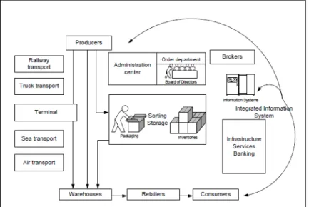
A logistics center is a defined area within which all activities relating to transport, logistics and the distribution of goods, both for national and international transit, are carried out by various operators. These operators can either be owners or tenants of buildings and facilities (warehouses, break-bulk centers, storage areas, offices, car parks, etc...) which have been built there.
Figure 1: An ideal logistic hub and its surrounding.
Source: (Skowron-Grabowska, 2008)
The example of an ideal logistic center is shown in the figure-1. Transportation, storage, packaging, labeling and other functions are concentrated in one place. Multimodal transportation can also be a part of the logistic center sometimes. In order to encourage intermodal transport for the handling of goods, a Logistics Centre should preferably be served by a multiplicity of transport modes (road, rail, deep sea, inland waterway, air).
5
The location of the logistics centers is a key element in enhancing the efficiency of urban freight transport systems and initializing relative supply chain activities sufficiently; thus, the location of an intermodal freight logistics center should be selected carefully; otherwise it may cause irreversible consequences in the city planning and also it may create bottlenecks that lead to rapid increase in cost in providing transport solutions (Europlatforms EEIG, 2004). All influencing factors for the determination of a location should be considered cautiously.
Finally, a Logistics Centre must comply with European standards and quality performance to provide the framework for commercial and sustainable transport solutions (Europlatforms EEIG, 2004).
The logistics hub can be distinguished by several ways depending on its usage. Depending on the location and geographical coverage, there are four kinds of logistics centers (Skowron-Grabowska, 2008).
1. International logistics centre: It consists with the highest degree of organizational and functional development in order to function on the vast international distribution networks with global range.
2. Regional logistics centers: Generally this type of logistics center the intermediary cells of regional and big-city distribution network;
3. Local distribution centers: Which constitute a point of gravity in local/city distribution network.
4. Industry distribution centers: Serve only one particular industry or single large company with specialized production range of products.
2.2. Factors affecting the location for a logistics hub
From the literature study and discussion with the experts in the field of logistics and location analysis, there are numbers of criteria identified for the evaluation of the location for logistics hub. The criteria can be classified by the two levels; main criteria and sub-criteria (which is underlying the main criteria). The major criteria can be infrastructure facilities, proximity to market, land availability, government and industrial support and labor supply (Lipscomb, 2010).
6 1. Infrastructure facilities:
Infrastructure facilities include the highways, railroads, and waterways and the existing airports and multimodal terminals in the region which can determine the capacity that any region/zone/city can handle. A region with better access to highways, railroads, etc. will be more capable of supporting new logistics developments (Lipscomb, 2010).
2. Proximity to Market:
This criterion considers the geographical market reach of a region. The proximity to market of any region can be described by how far the region can cover within a certain time by a specific mode of transportation. Besides it can also considers how many population can be served from a specific region within a certain time by specific mode of transport. According to (Lipscomb, 2010) a truck can reach approximately 600 miles each day , so the proximity to market for a region can be determined by how many regions or how many people are likely to serve within one day by truck.
3. Land Availability:
The development of new logistics hubs requires availability of unused land. This criterion considers the ability of a region to expand by horizontally. A new logistics development will likely require more land and infrastructure. This criterion can be measured by classifying the land of a region then identifying how much land can be used for the development of a logistics hubs. Moreover, the land value also determines indirectly the availability of land, if the land price is low, the more likely it is to be unused and which is the key for the company to develop a new logistics hub.
4. Government and Industry support:
Government and industrial support also requires for developing a new logistics hub. This criterion can be measured by the level of support that can get from both regional development authority and local industry. The more support a logistics hub gets from the government authority the more likely it is to be established.
Industrial development can be measured based on the existence of logistics development organizations in the region and the supporting logistics industry, i.e. distribution centers and warehouses.
7 5. Labor Supply:
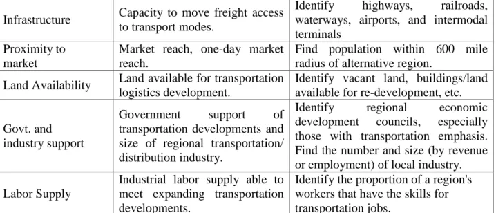
The availability of labor supply takes into account the regional demography databases. Generally the zones that are made up mostly of industrial laborers and have a history of industrial development. The regional demographic information can be collected from the ‘Statistiska Centralbyrån’, in Sweden to know about the employment characteristics of any region. From the employment characteristics data, we can get how much skilled or unskilled labor working in a region in different industry. The table 1 shows briefly the assumption of major criteria and their respective measurement method.
Table 1: Assumption and measurement method of location selection criteria for logistics hub
Criteria Assumption Measurement Method
Infrastructure Capacity to move freight access to transport modes.
Identify highways, railroads, waterways, airports, and intermodal terminals
Proximity to market
Market reach, one-day market reach.
Find population within 600 mile radius of alternative region.
Land Availability Land available for transportation logistics development.
Identify vacant land, buildings/land available for re-development, etc. Govt. and
industry support
Government support of transportation developments and size of regional transportation/ distribution industry.
Identify regional economic development councils, especially those with transportation emphasis. Find the number and size (by revenue or employment) of local industry. Labor Supply
Industrial labor supply able to meet expanding transportation developments.
Identify the proportion of a region's workers that have the skills for transportation jobs.
Source: (Lipscomb, 2010)
Besides these major factors, (Botha & Ittmann, 2008) identifies some other sub-attributes to consider for the evaluation of the location for logistics hubs;
Adequate multimodal transfer systems Good telecommunication systems Reasonable port charge
Adequate cargo and container handling facilities
Capable of handling all kinds of commodities (Including dangerous goods) Available rail and road links with local consumer and industrial areas
8
In addition, there are some other studies which explores some other different sub-factors to consider; (Botha & Ittmann, 2008)
Vehicle taxes
Road density and congestion Road infrastructure
Road and Bridge condition
Location away from residential zones and so on.
The decision about location of logistics centre should be made after a thorough analysis of the following factors: (Skowron-Grabowska, 2008)
Costs of labor in the given region, Costs of warehousing and transport,
Required level of service, i.e. a time from placing an order to delivery of the product to the customer (for instance 24 hours),
Taxes and customs duties. 2.3. Multi-criteria decision models
Decision making and analysis is an important part of the any kind of sciences since perhaps as old as mankind. Now-a-days, in many real world problems, the decision makers would like to consider more than one criteria or objectives to find out the goal of the study. This kind of decision making problems underlies in one broad category, called multi-criteria decision making (MCDM) problems (Farahani et al, 2009). Multi-criteria decision making can be defined as the evaluation of the alternatives for the purpose of selection or ranking, using a number of qualitative and/or quantitative criteria that have different measurement units.
There are many decision making problems regarding to spatial or geographical which is called location decisions. The term can also be used as; facility location, location science and location model. Facility location is more specifically related to locating or positioning at least a new facility among several existing ones in order to optimize (minimize of maximize) at least one objective function, for instance; cost, profit, travel distance etc.
9
Most of the literature includes the location model based on application-oriented solution procedures that are practical to handle large real world problems but rarely considered complexity or conflicting objectives. Secondly, the models were observed only the quantitative factors which are not incorporated with any qualitative factors for location decision models. But, now-a-days, in many cases, qualitative factors are the primary concern for the decision makers. Determination of where to locate the fixed facilities, for instance; logistic hub, depends upon a set of tangible and intangible criteria that are unique to a given problem. The traditional cost minimization or profit maximization models are not so appropriate, especially from the perspective of today's energy and environmental conscious era that we live in.
One analytical approach, suggested for solving such a complex problem is the Analytic Hierarchy Process (AHP), first introduced by Saaty (1977 and 1994). A review of state of the art models show that AHP method is able to reach the goal better than the other methods and this method can handle both qualitative and quantitative information at the same time when comparing with the other methods (Eskilsson and Hansson, 2010).
2.4. The SAMGODS Model: A brief overview
The Swedish national freight model systems (SAMGODS), is formulated for simulating the goods transportation (Jong et al, 2010)
In short run: representation of the base year, transport policy simulations.
In long run: forecasting scenarios, providing input for the assessment of the infrastructure projects.
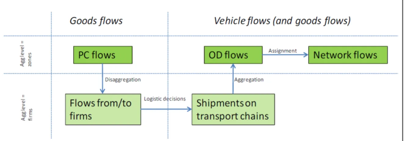
The SAMGODS model was implemented in a STAN program environment before 2005. Previously, the model had no logistic elements i.e. the determination of shipment size, the use of consolidation and distribution centers (Jong et al. 2002). Since 2005, the new model has been introduced to the real world problems but still there are some investigations going on to improve this model (Karlsson et al. 2012). The new Swedish freight model system, which includes the logistics model, is described by an aggregate-disaggregate-aggregate (ADA) model system (Fig-2).
10
Figure 2: Structure in SAMGODS model system
Source: (Karlsson et al. 2012)
The schematic figure-2 represents the structure of the SAMGODS model system, where the top layer includes the aggregate models and the bottom layer includes the disaggregate models. The model is also divided by the two levels of flows; goods flows and vehicle flows. The initial step, Production-Consumption (PC) flows comprise of determining the freight demand between production and consumption zones (also including the intermediate whole-sales zones, W). There are 34 different commodity types selected for determining this demand of goods (transport in, to, from and through Sweden). Then these production-wholesale-consumption (PWC) matrices are disaggregated by dividing the demand into small, medium and large firms. In the second step, the logistics decision are modeled i.e., optimal shipment sizes and transport chains, considering transport mode. In the third step, the consolidation (different firms) of shipments occurred and collected into Origin-Destination (O-D) flows of vehicles or goods. The vehicle flows are assigned to the individual network at last.
2.4.1. Commodity Flow survey
The commodity Flow Survey has carried out by SIKA, The traffic administration and the board of communications in 2001. The purpose of the survey is to collect the data of the commodity flows inside Sweden and between Sweden and other countries which is the main input of the base matrices in the SAMGODS model system (Jong et al. 2002). The survey provides information of i.e. origin and destination of type of commodities, their volumes, their values, transport modes etc. Later on the commodity flow survey (CFS) 2004/2005 (Edwards et al., 2008) and CFS 2009 (Trafikanalys, 2010) have been undertaken for SAMGODS model.
11 Administrative Zones:
There are total 464 regional administrative zones in the Swedish base matrix for SAMGODS model (which comes directly from the STAN-model). Among these 290 zones are domestic municipalities inside Sweden and 174 zones are foreign (covering all other countries). The foreign zones are widely spread in all over the world where the zones inside Europe has more zones than the other parts of the world considering the significant trade of that countries/regions with Sweden.
Commodity Groups:
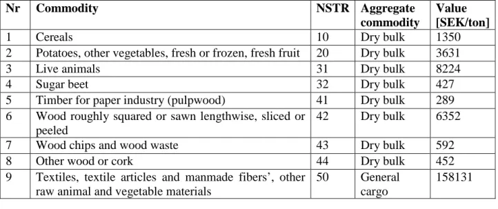
The logistics model in SAMGODS is working with the aggregated commodity groups, based on the standard NST/R1 commodities used in European statistics. The table is showing the commodity classification including the aggregation of commodity. All commodities are classified with different aggregate commodity types, i.e. dry bulk, liquid bulk and general cargo based on the specific logistic requirements. The value of the commodities is expressed by SEK/ton on the basis of year 2004 prices (excluding taxes), which are derived from the base matrix project (Edwards et al., 2008). Besides, the commodity number 30 (Mixed and part load, miscellaneous articles) hasn’t been used in the logistics model (Vierth et al, 2009). Therefore, mixed commodity transport cannot be considered in this study.
Table 2: Aggregate Commodity types for the SAMGODS logistics model
Nr Commodity NSTR Aggregate
commodity
Value [SEK/ton]
1 Cereals 10 Dry bulk 1350
2 Potatoes, other vegetables, fresh or frozen, fresh fruit 20 Dry bulk 3631
3 Live animals 31 Dry bulk 8224
4 Sugar beet 32 Dry bulk 427
5 Timber for paper industry (pulpwood) 41 Dry bulk 289
6 Wood roughly squared or sawn lengthwise, sliced or peeled
42 Dry bulk 6352
7 Wood chips and wood waste 43 Dry bulk 592
8 Other wood or cork 44 Dry bulk 452
9 Textiles, textile articles and manmade fibers’, other raw animal and vegetable materials
50 General cargo
158131
1 Nomenclature uniforme des marchandises pour les statistiques des transports (Standard Goods Classification for Transport Statistics)
12
10 Foodstuff and animal fodder 60 General
cargo
19558 11 Oil seeds and oleaginous fruits and fats 70 Liquid bulk 2576
12 Solid mineral fuels 80 Liquid bulk 713
13 Crude petroleum 90 Liquid bulk 2576
14 Petroleum products 100 Liquid bulk 3309
15 Iron ore, iron and steel waste and blast-furnace dust 110 Dry bulk 496
16 Non-ferrous ores and waste 120 Dry bulk 7444
17 Metal products 130 General
cargo
9762 18 Cement, lime, manufactured building materials 140 Dry bulk 2169
19 Earth, sand and gravel 151 Dry bulk 74
20 Other crude and manufactured minerals 152 Dry bulk 1114
21 Natural and chemical fertilizers 160 Dry bulk 2020
22 Coal chemicals 170 Liquid bulk 1210937
23 Chemicals other than coal chemicals and tar 180 Dry bulk 15959
24 Paper pulp and waste paper 190 Dry bulk 2155
25 Transport equipment, whether or not assembled, and parts thereof
200 General cargo
70281
26 Manufactures of metal 210 General
cargo
21041
27 Glass, glassware, ceramic products 220 General
cargo
15183
28 Paper, paperboard; not manufactures 231 Dry bulk 4637
29 Leather textile, clothing, other manufactured articles than paper, paperboard and manufactures thereof
232 General cargo
24920 30 Mixed and part loads, miscellaneous articles 240 General
cargo
19521
31 Timber for sawmill 45 Dry bulk 356
32 Machinery, apparatus, engines, whether or not assembled, and parts thereof
201 General cargo
47132 33 Paper, paperboard and manufactures thereof 233 General
cargo
15894
34 Wrapping material, used 250 Dry bulk 2250
35 Air freight (2006 model) General
cargo
561026 Source: (Vierth et al, 2009).
2.4.2. Logistics model output
This model generates a huge level of output files mainly grouped by a program to generate the available transport chains from origin to destination that is called Buildchain and a program for
13
the choice of the optimal shipment size and optimal transport chain which represents as
Chainchoi in the SAMGODS model.
The BuidChain folder contains the different output files containing the determination of transport chain per commodity shipments. The output files represent the best possible/ cheapest/shortest transport chain per commodity group and chain type, for every origin – destination pair.
The output from Chainchoi represents the optimization of the size of shipments and transport chain whereas the size of shipment is optimized by the capacity and merging with the similar kind of goods. It computes the optimal transport solutions (flows) for a selected commodity in a selected transport chain. The vehicle flow then assigned to a particular transport chain type which is the best transport chain from origin to destination. The different output files contain a number of quantities for the chain: total flow between the zone, number of shipments, various types of costs including transport cost and total logistics cost from origin to destination. The transport cost is calculated by the model including the loading and unloading cost for each commodity group.
2.5. The Accessibility measure
In general, people and different activities will prefer different locations based on the location’s attractiveness for a particular type and scale of activity and the accessibility of that particular location (Meyer & Miller, 2001). ‘Attractiveness’ of a location for an activity depends upon a number of different factors such as, the attractiveness of any neighborhood as a residential area depends on, the price, size, type, age, quality of the available housing and so on (Meyer & Miller, 2001). ‘Accessibility’ is determined by the spatial distribution of potential location, the ease of reaching each destination and the magnitude, quality and the character of the activities found there (Handy & Niemeier, 1997). However, the two most fundamental questions concerning accessibility measures are for whom and for what, and the most straightforward description of accessibility is the state of connectivity (Baradaran & Ramjerdi, 2001). Moreover, an accessibility measure is a powerful tool for determining the need and the effectiveness of a land use whether it can be used as a certain purpose or not.
The measures of accessibility mainly consist of two parts: an attraction/activity element and a transportation element (Handy & Niemeier, 1997). The activity/attraction element considers the
14
spatial distribution of particular activities, for example, location of shopping centers which attracts people. This can also be represented as attractiveness of a location for a particular activity. Besides, the transport element considers the easiness of travel between the locations and can be measured by travel distance, time or cost.
Accessibility can be measured by generally three different methods: Cumulative opportunity method
Gravity-based method Utility-based method
Gravity-based method
The gravity-based measure developed by (Hansen, 1959) is still the most widely used general method for measuring accessibility which is also called the potential location accessibility measure. This gravity based accessibility measure can be expressed as follows; (El-Geneidy & Levinson, 2006)
Where, Ai is measures of accessibility from zone i to all opportunities (D) in the different zones j,
15
CHAPTER 3: METHODOLOGY OF THE STUDY
This chapter presents the research methodology used in this thesis. The research methodology is described briefly step by step here.
Step 1:
The first stage, the goal, purpose and objectives of this research have been identified which I already described in Chapter 1.
Step 2:
This research is initialized by an extensive literature review of the existing research on the logistics location analysis. From the literature review it is trying to find out what are the criteria to evaluate the location for logistics hub, which is one of the objectives in this research. Besides, the literature review reveals a lot of multi-criteria decision models (MCDM) to evaluate the location for logistics hubs.
Figure 3: The methodology flow chart
Step 1: Finding the goal of the study
Step 2: Literature review
Step 3: Multi-criteria Location Decision Models
Step 4: Data Collection and Preparation
Step 5: Case study Results, Analysis and Discussion
Step 6: Conclusion and Recommendation AHP
Method
Gravity Method
16 Step 3:
There are two different multi-criteria decision models (MCDM) that have been applied in this research. The first model applied for this research is Analytic Hierarchy Process because of its wide range usage in this research field. The AHP model considers several criteria to evaluate the location for logistics hub which will be described later on the chapter 4 in detail. Later on a simple gravity model is used in this research as well to find out the attractiveness of logistics hub location. For this model, I only consider certain commodity types, excluding mainly oil and timber shipments. The accessibility measures by considering the data of flow of logistics goods and respective transport cost. However, these two models are presented separately in this thesis in order to avoid the double counting of the criteria considering the location selection for logistics hubs.
Step 4:
There are a lot of data required for both models. Both primary and secondary data is used for this research. The data collected from different sources as well. Some of the criteria data comes from the secondary sources. And others come from the output of SAMGODS logistics model 2.02 conducted by VTI in 2009 based on the Base matrix data.
The second part of the approach is to get expert’s opinion and data collection from the questionnaire survey. Moreover, one criteria data is found from the company Brinova.
Step 5:
Results and discussion from both models represents in this step. The result from the AHP method is based on the judgment of decision makers. And the gravity model output is based on the factors considered calculating the level of accessibility for a location.
Step 6:
Finally from the results of both models, recommendation and conclusion have been drawn.
17
CHAPTER 4: AHP METHOD AND A CASE STUDY
In this chapter the method of Analytic Hierarchy Process (AHP) is described briefly. Then the method is applied in a case study for Brinova. The result from the case study is illustrated in this chapter.
4.1. The AHP method
The Analytic Hierarchy process (AHP) is a multi-criteria decision making method developed by Saaty, (1980). The AHP model is used because it can handle dynamic and complex real world multi-criteria decision-making problems (Yang & Lee, 1997). The method can handle both tangible and intangible factors at the same time affecting the evaluation of location-based problems as well (Regmi & Hanaoka, 2011). AHP allows decision makers to model a complex problem in a hierarchical structure, showing the relationships of the goal, objectives/ Criteria, and the alternatives (Adamcsek, 2008). The AHP is based on three basic principles which are described as follows.
4.1.1 Problem Decomposition
The decomposition principle is useful to structure a complex problem into a hierarchy of clusters. The objective or overall goal of the study is represented at the top level of hierarchy. The criteria and sub-criteria to achieve the goal or objective are represented at the intermediate levels. Finally the decision alternatives or selection choices are laid down at the bottom layer of the hierarchy.
Figure 4: General structure of Analytic Hierarchy Process (AHP)
The main goal of the study stands at the top of the hierarchy while the decision alternatives are at the bottom which is shown by the above figure 4.
18 4.1.2. Comparative analysis
If the hierarchy has been structured, the next step is to determine the priorities of elements in every level of hierarchy. The relative importance of each element at a particular level will be measured by a fundamental rating scale for pair-wise comparison (Saaty, 1980). The decision makers provide numerical values for the priority of each element according to the Saaty rating scale (Table 3). The pair-wise comparisons are given in terms of how much element ‘i’ more important than element ‘j’. These priority weights obtained from the questionnaire survey to the decision makers.
Table 3: The fundamental scale (modified from Saaty, 1980)
Score Relative importance
1 Objectives i and j are of equal importance.
3 Objectives i is weakly more important than j.
5 Objectives i is strongly more important than j.
7 Objectives i is very strongly more important than j.
9 Objectives i is absolutely more important than j.
2,4,6,8 Intermediate values
Reciprocals
If activity i has one of the above numbers assigned to it when compared with activity j, then j has the reciprocal value when compared with i.
This relative importance/scoring within every level of hierarchy will result in a matrix of scores, 𝐴 = �𝑎𝑖𝑗�, 𝑎𝑖𝑗 > 0 𝑎𝑛𝑑 𝑎𝑖𝑖 = 1
19
In general it produces square and reciprocal matrices from the wise comparison. The pair-wise comparison matrix can be represented as follows:
𝐴 = �𝑎11⋮ ⋯ 𝑎⋱ 1𝑛⋮ 𝑎𝑛1 ⋯ 𝑎𝑛𝑛
�
Where, 𝑎𝑖𝑗= 1
𝑎𝑗𝑖 , ∀ 𝑖, 𝑗
From the comparison matrix, we can get the Eigenvector of single priority of every element by the following way of Eigenvector method. This method suggested by Saaty, (1980) to measure the vector of weights for every element, (w1, w2, w3 ……)
Again, A= � 𝑤1 𝑤1 ⋯ 𝑤1 𝑤𝑛 ⋮ ⋱ ⋮ 𝑤𝑛 𝑤1 ⋯ 𝑤𝑛 𝑤𝑛 � × �𝑤⋮1 𝑤n � = n �𝑤⋮1 𝑤n � [1] Where, 𝑤𝑖𝑗= 1 𝑤𝑗𝑖 , ∀ 𝑖, 𝑗
The above equation can be simply described as;
𝐴 ∗ 𝑤 = 𝑛 ∗ 𝑤
Where A is the comparison matrix, w is the eigenvector and n is the dimension of the matrix. By the above eigenvector method, the priority vector from the pair-wise comparison of each level is measured.
4.1.3. Synthesis of priorities and the measure of consistency:
The pair-wise comparisons from each level of hierarchy generate a matrix of relative rankings. The number of matrices depends on the number of the elements on each level in the hierarchy. The priority weights of the elements will be computed using eigenvector or least square analysis. The process is repeated for each level of the hierarchy until the goal has been achieved by overall composite weights.
20
In the final stage it is necessary to calculate the Consistency Ratio to measure how consistent the judgments compare to large samples of purely random judgments (Adamcsek, 2008). According to Saaty, (2003) the largest Eigen value (𝜆 𝑚𝑎𝑥) is equal to the number of comparisons. So, the equation [1] can also be simplified as;
𝐴 ∗ 𝑤 = 𝜆 𝑚𝑎𝑥∗ 𝑤
Where, 𝜆 𝑚𝑎𝑥 = largest Eigen value.
Saaty, 1980 mentioned a measure of consistency, called Consistency Index (CI) which is defined as the following;
Consistency Index (CI) = 𝜆 𝑚𝑎𝑥− 𝑛
𝑛−1
Finally the Consistency Ration (CR) is calculated by using the following equation; Consistency Ration (CR) = CI
RI
Where, RI represents as Random Index which is depending on the value of n. In addition, Saaty (1977) simulated the random pair-wise comparisons for different size matrices, calculating the consistency indices. The following table-4 represents the random consistency index with respect to the size of the matrix.
Table 4: The average Consistencies of random matrices (RI values)
Size 1 2 3 4 5 6 7 8 9 10
RI 0.00 0.00 0.58 0.90 1.12 1.24 1.32 1.41 1.45 1.49
Source: (Saaty, 1977)
In general, CR value less than 0.10 is acceptable for the judgments but if the value is higher, the judgments may not be reliable and then need to carefully review again.
21 4.2. Data Collection for AHP method
The method requires data to apply AHP in a case study. AHP data collection includes with the quantitative data from mostly secondary sources and survey of the decision makers. In the case study, the decision makers judge the pair-wise comparison on the basis of this secondary quantitative data. And the survey data from decision makers are collected later on to finalize the ranking for the evaluation of logistics hubs.
4.2.1. Secondary Data:
The criteria data for the case study are obtained from several secondary sources. All the data are quantitative so that the preferences were judged by the decision makers are consistent. The criteria data of port capacity is collected from the Swedish port authority database per year in 2011, which has the data of yearly goods transshipment through different ports in Sweden (Sveriges Hamnstatik , 2011). For Stockholm I just sum up the data from all the ports in greater Stockholm. The intermodal capacity data has also collected from the secondary source (appendix-2).
4.2.2. Primary/Survey data:
To collect the survey data, firstly I selected the decision makers (evaluators) those who are knowledgeable in this field of study. After that they were asked to conduct a survey of the pair-wise comparisons in the AHP model. The survey sheet for pair-pair-wise comparison matrices are in the appendix-2. As there are only three decision makers for the evaluation of the AHP matrix, I tried to find out all the judgments from all decision makers. Besides the decision makers got all the freedom to give the preferences, as they are not from any company, their evaluation is based on their experience and perception in this field.
22 4.3. Application of AHP method: A case study 4.2.1. Problem Decomposition
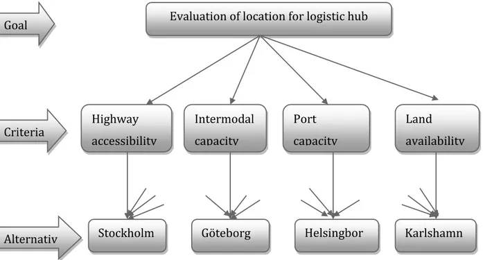
The hierarchy consists of the main goal is at the top of hierarchy, and then criteria for reaching the goal and finally selection of different alternative locations are at the bottom. The decision makers have prioritized the two level of hierarchy by the fundamental scale for relative judgment. Firstly, the pair-wise comparative analysis between the criteria to achieve the goal and secondly the pair-wise priorities between the alternatives with respect to the different criteria. In every step of comparison matrices, the consistency index and ratio is calculated due to show the validation of the judgments. At last all of the priorities from the two pair-wise comparisons are being synthesized by a composite matrix calculation where the final decision will be achieved. For the case study, the hierarchy tree of AHP can be drawn by the following Figure 5.
Figure 5: The AHP hierarchy for evaluating the location for logistics hubs
Evaluation of location for logistic hub
Highway accessibility Intermodal capacity Port capacity Land availability
Stockholm Göteborg Helsingbor Karlshamn
Goal
Criteria
23 Criteria Selection:
The literature review of factors affecting the location for logistics hubs explored different criteria for the evaluation of logistics hubs. But most of the factors are considering economic factors or efficiency of using the logistics hubs. Besides, this study is limited to evaluate the locations for the logistics hubs not how efficiently a hub can be used. However, the environmental impact is considered indirectly in this study with the expert’s opinion by minimizing the criteria weight of the highway accessibility and maximizing the weight for other criteria i.e., intermodal capacity, port capacity or land availability. From the literature review and opinion of the experts, the following criteria are selected regarding the evaluation of location for logistics hubs in Sweden (Table 5).
Table 5: Assumption of the factors for evaluating the location for logistics hubs
No. Factors Assumption
C1 Highway Accessibility Number of major highway connected with the zone.
C2 Intermodal Capacity Number of intermodal terminals and their capacity by number of railway tracks, handling goods capacity etc.
C3 Port Capacity Number of ports and their frequency of shipment per year. C4 Land availability Average land value or rent per square meter.
Alternative Selection:
The selection of alternative locations is based on the interest of Brinova, which are options for decision making. With the consultation of Brinova, I selected these four locations; Stockholm, Göteborg, Helsingborg, Karlshamn. Brinova has their own logistics center in southern part of Stockholm and Helsingborg but not any logistics center either in Göteborg or Karlshamn. However, the geographical position of these locations is vital for this study, whereas all the locations can be accessed by sea transport which is very important characteristics for a logistics hub.
4.2.2. Comparative Analysis
Step 1: Criteria vs. Criteria pair-wise comparison:
Based on the rating scale from 1-9, the initial ratings of the decision maker’s pair-wise comparison of criteria vs. criteria are evaluated. The criteria listed on the left column are one by
24
one compared with every criteria listed on the top row. Here, the decision makers are judging which criterion is more important with respect to the goal of selecting the location for logistics hubs. Matrices were produced from three different expert’s judgment (appendix-2).
The representation of the overall derived priority weight calculation from the initial ratings/judgments by the decision makers is also in appendix-3 by the Eigen Vector method. As the decision makers were asked to judge these pair-wise comparisons by their own point of view, these makes for some dissimilarity of judgment.
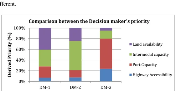
Comparison between individual priorities:
There are some significant differences found from the individual ratings due to the decision makers perspectives are different in point of view. Here, Figure 5 illustrates there are some major variations of expert’s judgments of the criteria for example, the priority of land availability differ from 0.05 to 0.41. Besides, one of them put more weight on intermodal capacity while others put more weight on land availability and port capacity which is clearly visible from the following fugure-6. Since the variation of relative preference is significant, it is likely that the final ranking will be different.
Figure 6: Comparison of Decision maker's priority between the criteria
Step 2: Criteria wise Alternative Comparison:
In this section, all the alternatives will be rated with respect to each criterion by the fundamental scale. In this case study, four alternatives and four criteria have been selected which I have already discussed. So, four different criteria produced four different initial pair-wise rating matrix from every decision maker which is shown in appendix- 4. Again by using Eigen vector
0% 20% 40% 60% 80% 100% DM-1 DM-2 DM-3 D er ived P rio rit y (% )
Comparison between the Decision maker's priority
Land availability Intermodal capacity Port Capacity Highway Accessibility
25
method, the final derived priority vector is calculated which is shown by the tables in appendix-5. In this case, the decision makers rating of individual alternatives priority is mainly based on the quantitative data that is collected from several secondary and primary sources (appendix-6). After applying the Eigen vector method, I can derive the priority weight of every alternatives based on a certain criterion.
Comparison between individual priorities:
From the previous step we already know about the criteria and now the criteria wise individual priority comparison will be discussed by the following graphs.
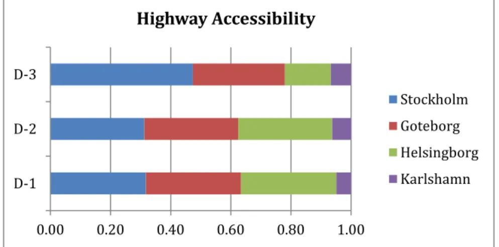
Criteria 1- Highway Accessibility
In this criterion, I only consider the major highway links connected to particular location/alternatives that we take into account for judgment. The figure 7 illustrates the derived priority from the initial ratings of the decision makers. Since the major cities like Stockholm and Goteborg have best highway communication system for transporting goods by road, so Stockholm and Goteborg got the highest priority from all the experts. The main three major European highways linked with these two major cities in Sweden. Whereas there is only one major highway connected with Karlshamn, therefore it gets the lowest ratings from the experts which is clearly visible by the below figure 7.
Figure 7: Derived priority of highway accessibility
Besides, Helsingborg is a vital strategic point for transporting goods to Denmark and vice versa, and there are two major European highways E4 and E6 linked with that. For this reason Helsingborg got nearly same weight as Stockholm and Goteborg.
0.00 0.20 0.40 0.60 0.80 1.00 D-1 D-2 D-3 Highway Accessibility Stockholm Goteborg Helsingborg Karlshamn
26
Criteria 2- Port Capacity
In port capacity, I consider the data of how much goods handled by the port per year. So it is obviously the highest priority given to the port of Goteborg because it is handling five or six times more goods per year than that of others (figure-8). All the major shipments both inbound and outbound to Sweden are using this port. While other ports that we are considering have got roughly the same priorities, as they are handling approximately same amount of goods per year.
Figure 8: Derived priority of port capacity
Criteria 3- Intermodal Capacity
The availability of Intermodal station considered firstly for this criterion and then characteristics of that intermodal station has been considered as assumption for the judgment. The characteristics of the intermodal station include; total terminal station, no. of rail tracks, depot capacity, reach stackers and so on. Based on this data of intermodal station, the experts set their initial pair-wise comparison between the alternatives that depicts by the following figure 9. Karlshamn has no intermodal station within their territory and for that reason it has got the lowest priority from all the decision makers. Moreover, other locations have their own intermodal stations which have more or less the same characteristics. So, the derived priorities of three regions are approximately same which represents by the figure 9.
0.00 0.20 0.40 0.60 0.80 1.00 D-1 D-2 D-3 Port Capacity Stockholm Goteborg Helsingborg Karlshamn
27
Figure 9: Derived priority of Intermodal Capacity
Criteria 4- Land Availability
The pair-wise comparison of alternatives with respect to land availability is considering the average land value or land rent. As the land rent or value is much higher in major cities, it is one of the disadvantages to establish a new logistics hub which brings the lower priority to the all major cities. On the contrary, Karlshamn is growing city with very low land value or rent and that brings the priority is much higher than the other cities by the decision makers.
Figure 10: Derived priority of Land availability
4.2.3. Final Weight of Alternative Selection:
After synthesizing all the criteria weight and alternative weight, I can get the final ranking by summing up the final priority getting from the step 1 and step 2 described previously. So the final priority of any location is the aggregate priority which can be represented by the following equation. 0.00 0.20 0.40 0.60 0.80 1.00 D-1 D-2 D-3 Intermodal Capacity Stockholm Goteborg Helsingborg Karlshamn 0.00 0.20 0.40 0.60 0.80 1.00 D-1 D-2 D-3 Land availability Stockholm Goteborg Helsingborg Karlshamn
28
𝐿1 = �(𝑓𝑖𝑛𝑎𝑙 𝑝𝑟𝑖𝑜𝑟𝑖𝑡𝑦 𝑜𝑓 𝐶𝑟𝑖𝑡𝑒𝑟𝑖𝑎 𝑤𝑖𝑡ℎ 𝑟𝑒𝑠𝑝𝑒𝑐𝑡 𝑡𝑜 𝑔𝑜𝑎𝑙 𝑖
∗ 𝑓𝑖𝑛𝑎𝑙 𝑝𝑟𝑖𝑜𝑟𝑖𝑡𝑦𝑜𝑓 𝐿𝑜𝑐𝑎𝑡𝑖𝑜𝑛 𝑤𝑖𝑡ℎ 𝑟𝑒𝑠𝑝𝑒𝑐𝑡 𝑡𝑜 𝑐𝑟𝑖𝑡𝑒𝑟𝑖𝑎)
The final result from the AHP evaluation is displayed by the following figure-11. Since the different decision makers judge the criteria differently, the result has got some variations of alternative ranking finally. Generally the comparative analysis of criteria (Step 1) determines the final priority since the alternative judgment was based on the quantitative data. It is obvious that Göteborg has got the highest ranking from all the decision makers’ point of view (figure 11). However, the value of final priority is changing among the decision makers and the difference between the other alternative clearly explains that Göteborg is the best location considering the criteria.
Figure 11: Final ranking of Alternative selection
Karlshamn is second position from the decision maker (DM-1) but got the lowest position (Fig-11) from the other decision makers because Karlshamn has got only advantage from lowest land value. On the contrary Karlshamn has no intermodal facilities and lower level of highway accessibility. 0.17 0.23 0.20 0.31 0.31 0.48 0.26 0.28 0.21 0.26 0.18 0.11 0.00 0.10 0.20 0.30 0.40 0.50 0.60 DM-1 DM-2 DM-3 Fin al p rio rit y
Final ranking of location selection
Stockholm Goteborg Helsingborg Karlshamn
29
CHAPTER 5: LOCATION-BASED ACCESSIBILITY
In this chapter the gravity method for measuring the accessibility of logistics hub location is described briefly. The result of this model is also presented in this chapter.
5.1. The Gravity method
A simple gravity based location model is used to conduct the quantitative analysis of attractiveness for all the alternative locations. The attractiveness for a logistic hub location depends upon several different factors which I already mentioned in the literature review chapter. However, in this research it is limited in terms of the number of attraction attributes that can be specified and observed. Here in this study, two most important variables are selected to determine the attractiveness of the location for logistics hubs; flow of goods and transport cost. Flow of goods means the logistics goods shipment in a year from one zone to another zone, where every municipality represents as one zone within Sweden. And the transport cost means the respective transport cost for transferring goods from one zone to another.
All the accessibility method has mainly two components; one is the attractiveness and other is the impedance function. The attractiveness is measured by number of opportunities/activity at any locations (El-Geneidy & Levinson, 2006). The impedance function considers the probability of attraction of those locations whereas the probability of attraction can be measured by the distance, travel time or transport cost between the zones. Therefore, the level of accessibility is expected to increase with the increasing number of opportunities/activities that can be reached from a location; however, accessibility will decrease with the increasing cost to get that opportunity/activity and vice-versa.
5.1.1. Model Assumption
The model is generalized by a decreasing exponential function of transport cost between the origin and destination. In this model, the attractiveness component measured by the flow of goods which is provided by the data of commodity wise O-D matrices from the SAMGODS model output (Vierth et al, 2009). And the impedance function is based on the negative exponential function of the transport cost between the origin and destination of flow of goods. The parameter (𝛽) denotes the sensitivity of transportation cost, which value should be positive. The larger the beta is in magnitude, the less likely transport flows are to go a long distance.
30
In this study the accessibility is measured by the following equation-[2]. 𝐀𝐢 = �(𝑶𝒋+ 𝑫𝒋) 𝒆−𝜷𝑪𝒊𝒋
𝒋
[𝟐]
5.1.2. Input variables and parameters Ai = Accessibility of location i.
Oi = Outbound/Export of total goods from zone i.
Dj = Inbound/ import of total goods in zone j.
𝛽 = Parameter indicating the sensitivity of transport cost. Cij = Transport cost between the location i and j [SEK/Ton].
Where, the export and import can be determined by the following two equations; the export (Oi)
is calculated by summing up all the flow of goods outgoing from zone i to all other zones j and import (Dj) is calculated by summing up all the good flows incoming from any zones i to a zone j.
By the following equation [3] and [4], the total outbound and inbound flow of goods is measured, where Tij is the total goods flow (in tons) from one municipality i to another j.
𝑶𝒖𝒕𝒃𝒐𝒖𝒏𝒅 𝒇𝒍𝒐𝒘, 𝑶𝒊= � 𝑻𝒊𝒋
𝒋 [𝟑]
𝑰𝒏𝒃𝒐𝒖𝒏𝒅 𝒇𝒍𝒐𝒘, 𝑫𝒋= � 𝑻𝒊𝒋
𝒊 [𝟒]
The first part of accessibility measurement is attractiveness which considers all the activities in a zone, measured by the flow of logistics goods to or from a certain zone. And the second part, the impedance function measures by the negative exponential function. The negative exponential function mainly considers transport cost between the zones and the parameter (𝛽). So it is expected that when the transport cost between two zones increases the accessibility decreases and vice-versa. However, the positive parameter (𝛽) indicates how sensitive the accessibility value is to the cost variable. If the beta value would be 0, then the transport cost between the zones would have no effect, the accessibility of the zones would only depend on the summation of the other zones goods flow. When the beta value increases the effect of the transport cost for calculating the accessibility will also be increased. Therefore, this model needs to have an accurate beta value. Finally the accessibility is calculated for any zone i by summing up total export and import goods of the other zones and considering the respective transport cost between the zones i and other zones j.
31 5.2. Data collection and preparation
The input data for the Accessibility measure by gravity model obtained from the SAMGODS logistics model output (Vierth et al, 2009) which is based on the Commodity flow survey 2001 and 2004/2005 data. The output from the SAMGODS model which I used in this research is called ‘Chainchoi’. The ‘chainchoi’ is the Samgods logistics model which gives information of optimal shipments sizes and transport chains per commodity wise, which I have already discussed briefly in the literature chapter. The output of logistics model delivers the information of flows of different commodities from origin to destination or senders to receivers.
5.2.1. Data preparation:
Since the study considers the Brinova’s perspective, the commodity has been selected with the consideration of their business area. In this gravity model, I only selected several commodities excluding mainly Liquid bulk i.e. oil and chemicals, timber and wood products. The commodity types have been selected by Brinova for the relevance of their business or which commodities they are interested to deal with. The following table is a subset of selected 10 commodity types from 35 aggregate commodity types used in SAMGODS.
Table 6: Selected Commodity types for the input of gravity model.
Nr Commodity NSTR Aggregate
commodity
Value [SEK/ton] 6 Wood roughly squared or sawn lengthwise, sliced
or peeled
42 Dry bulk 6352
9 Textiles, textile articles and manmade fibers’, other raw animal and vegetable materials
50 General cargo 158131
10 Foodstuff and animal fodder 60 General cargo 19558
17 Metal products 130 General cargo 9762
18 Cement, lime, manufactured building materials 140 Dry bulk 2169
26 Manufactures of metal 210 General cargo 21041
27 Glass, glassware, ceramic products 220 General cargo 15183 29 Leather textile, clothing, other manufactured
articles than paper, paperboard and manufactures thereof
232 General cargo 24920
32 Machinery, apparatus, engines, whether or not assembled, and parts thereof
201 General cargo 47132 33 Paper, paperboard and manufactures thereof 233 General cargo 15894 Source: (Vierth et al, 2009).
32 5.3. Determination of Beta value
The value of beta 𝛽 must be calibrated for use of gravity model (Ortúzar & Willumsen, 2001). In order to determine the beta value for accessibility measure, it is assumed the choice of any destination (j) depends on the utility of that zone where the utility of a destination measures by the transport cost between locations. As we already know the data of total incoming and outgoing shipments for every zones and the cost of respective shipments, we can determine the value of beta by the following equation [5]. The left part of the following equation considers summation of the goods flow between all zones and their respective transport cost.
� � 𝑻𝒊𝒋 𝒋 𝑪𝒊𝒋 𝒊 = � 𝑶𝒊 𝒊 � 𝑪𝒊𝒋∗ 𝑷𝒊𝒋 𝒋 [5] 𝑾𝒉𝒆𝒓𝒆, 𝑷𝒓𝒐𝒃𝒂𝒃𝒊𝒍𝒊𝒕𝒚 , 𝑷𝒊𝒋 = 𝑫𝒋𝒆 −𝜷𝑪𝒊𝒋 ∑ 𝑫𝒌 𝒌𝒆−𝜷𝑪𝒊𝒌
The right hand side of the equation [5] considers the outgoing total flow from an origin (outbound) and cost parameter multiply with the probability to choose a destination. The probability is calculated by Multinomial Logit Model considering the utility of any destinations by the transport cost between the zones. We have only unknown value in this equation is beta. The flow chart of determination of beta value is illustrated in figure 12. Visual C# coding (appendix-7) is used to solve these equations [2], [3], [4] and [5] and determine the beta value to compute accessibility for all municipalities in Sweden. Moreover, the flow chart (figure-12) also shows how the output: level of accessibility (Ai) is measured from the equation [2]. First of all
the input data of O-D flows per commodity wise is collected from SAMGODS model output which will be described briefly next in data collection and preparation paragraph. From that dataset I need only the transshipment volume and respective transport cost from origin to destination. Then 4th step, I calculated the total flow of goods by summing up all the shipments throughout the year from one municipality (i) to another (j) considering all selected commodity types (table-6). The transport cost between one zone to another taking into account only when the flow between zones greater than zero otherwise the cost set to be zero and which is not counted to compute the level of accessibility (5th step). In 6th is for computing the transport cost (SEK/ton) from one zone (i) to another (j) whereas in 7th step is for computing inbound and outbound flows by equation [3] and [4], the unit is tons.
33
Figure 12: Flow chart of determination beta value and Accessibility
The beta value is computed from the difference between the LHS and RHS in the equation [4], where RHS value is changing with the changing of beta value. For assuming a beta value, when the difference between LHS and RHS is the lowest, I took that value for computing the accessibility. The value of beta finally came ‘0.01823’. It seems that the beta value is close to zero. Depends on the scale used for 𝐶𝑖𝑗 the impact of beta value in this model is lower. In final step I got the accessibility from the equation [2] which is described earlier in this chapter.