The decoupling process of CO2 emissions and economic growth : A comparative study between the European Union and middle income countries in South and East Asia

The decoupling process of CO

2

emissions and economic growth:

A comparative study between the European Union and middle

income countries in South and East Asia.

BACHELOR

THESIS WITHIN: Economics

NUMBER OF CREDITS: 15

PROGRAMME OF STUDY: International Economics AUTHOR: Elin Alverhed and Frida Kåvik

JÖNKÖPING May 2020

Bachelor Thesis Degree Economics

Title:

The decoupling process of CO2 emissions and economic growth: A comparative study between the European Union and middle income countries in South and East Asia.

Authors:

Elin Alverhed and Frida Kåvik Tutor: Anna Nordén Date: 2020-05-18

Key terms: Development, CO2 Emissions, South and East Asia, The European Union, Decoupling

This paper compares and analyzes the decoupling processes of carbon emissions to economic growth in the European Union and South and East Asian middle income countries. This is done through econometric methods, testing for a relationship between CO2 and GDP. The study is conducted by first testing for the hypothesis that there is a significant difference of the turning points between the EU and the Asian region, and thereafter if there is a significant difference in the decoupling processes. The findings show that the Asian middle income countries have a lower turning point than the EU. It is also found that the EU experienced absolute decoupling in 2014, whereas the Asian countries only experienced weak relative decoupling. The study is based on four theories; The Environmental Kuznets curve, Tapio’s Decoupling model Theory, Rostow’s Stage of Growth Theory and the Ecological Modernization Theory. The findings, together with the theories, show that improved technology, together with implementations of international policies, can have positive effects on environmental changes.

Table of Contents

1.

Introduction ... 1

2.

Theoretical Framework ... 6

2.1 The Environmental Kuznets Curve ... 6

2.2 Tapio’s decoupling model theory ... 7

2.3 Rostow’s Stage of Growth Theory ... 8

2.4 The Ecological Modernization Theory ... 9

2.5 Previous Empirical Findings ... 10

3.

Empirical Framework ... 12

4.

Discussion... 22

5.

Conclusion ... 25

6.

Reference list... 26

7.

Appendix ... 30

7.1 Tables and graphs... 30

7.2 Outputs from EViews ... 31

1. Introduction

Global climate change is affecting countries worldwide. The priority to change human behavior and the concern of how the climate is affected by our way of living has risen tremendously in recent years, particularly in high income countries (Sanyé-Mengual et al., 2019). Still, it is a split debate with some constantly trying to find solutions and some denying the very existence of the problem. Currently, different countries experience various stages of development, therefore the ability to contribute to change differ among nations. In the developed world, it is easier to use methods to cut emissions, trying to be more sustainable, whereas for less developed countries, this is not a top priority (Mulvaney, 2019). A theory that supports this behavior is the Environmental Kuznets curve, which indicates that when an economy develops, environmental degradation initially increases and thereafter decreases (Dinda, 2004). In this paper, the decoupling process of carbon emissions in the European Union will be analyzed and compared to the decoupling process of middle income countries in South and East Asia. Decoupling is evaluated through testing whether the EU, or the Asian countries experience decreases in environmental degradation, and increases in economic growth in terms of GDP simultaneously, much like the Environmental Kuznets curve indicates after its turning point (Dinda, 2004)1.

Building on the theory of the Environmental Kuznets curve, this paper is a comparative study where trends in carbon emissions in the two regions are analyzed, two regions currently experiencing different stages of economic growth. According to the European Commission (2018), the EU has previously claimed that they have decoupled their economy from carbon emissions in relation to economic growth (European Commission, 2018), a statement that will be tested in this paper. The results will later be compared to the South and East Asian middle income countries in order to see if they are experiencing a similar decoupling trend. A list with all countries included in each region can be seen in Appendix 7.1.1. An analysis of the differences between the two regions is interesting as the European Union consists of mostly high income countries whereas the Asian region only consists of middle income countries. The differences in economic growth will potentially show differences in levels of emissions and in turn decoupling processes. Will the Asian region follow the same path as the EU, or will today's increased technological effects change the pattern of environmental

degradation for less developed nations? If the results indicate a difference in the decoupling process between the two regions, the theories of Ecological modernization and Rostow’s stages of growth will be used to analyze the decoupling trends and potentially explain why a difference can be seen.

The European Union and many of the Asian middle income countries taken into account in this study, all aspire to reach environmental goals to reduce their effect on environmental degradation. Although in 2016, the EU had reduced their greenhouse gas emissions by 24 per cent relative to 1990, in more recent years this decrease has not been as prominent. China on the other hand, one of the countries included in the Asian region has previously not aspired to reach the same targets as the EU. Their greenhouse gas emissions have grown tremendously for more than three decades, however, the increase started to diminish in 2011 (World Bank, 2019). As the greatest emitter of greenhouse gas emissions in the world, actions taken by China have enormous consequences on the world's total emissions, but evidently recent policies have made a difference (World Bank, 2019).

China, as of the most influential countries in the Asian region, with a fast growing economy, will potentially sway the path for improvements in many other countries in the region. As most of these middle income countries are net exporters of production as opposed to most of the European countries, implementations applied to decrease environmental degradation will most likely make a larger difference here ("CO₂ emissions embedded in trade", 2020). A reason for this is that most technological changes are relatively more beneficial to improvements within production than for consumption (Kuroda, 1989), hence decoupling will potentially occur at a lower level of economic growth in the Asian region than in the EU. Middle-income countries in Asia are the most prevalent in this region, representing the predominant percentage of the population. Are the trends in the decoupling process of carbon emissions and economic growth in the two regions the same, or can the potential differences be explained by other factors and theories?

1.1 Background

The European Union and many of the Southern and Eastern Asian middle income countries analyzed in this study, have initiated sustainable investments and future goals to decrease emissions. The EU is to reduce their greenhouse gas emissions by at least 40 percent by 2030 relative to 1990 (Intergovernmental Panel on Climate Change, 2006). According to The

International Energy Agency, the EU has also promised to reduce their emissions by 20 per cent by 2020 and further by above 80 per cent by 2050 (Intergovernmental Panel on Climate Change, 2006). However, as previously mentioned, the decrease in environmental degradation has not been as prominent in recent years. Similarly, investments and goals have been made for the Asian economies. In recent years, China has started investing heavily on renewable energy, aiming to reduce their reliance on fossil fuels such as coal. In 2005 China's renewable energy investments accounted for around $2 billion USD, whereas in 2011 it accounted for as much as $51 billion. Seemingly, China has set some of the world's most ambitious targets concerning renewable energy. Of these $51 billion, 87% represented photovoltaic and wind energy (Ming et al., 2014). Such investments are essential for promoting clean energy innovation, as the benefits contribute to cleaner air, less greenhouse gasses and thus, better living standards.

Many of the other middle income countries in Southern and Eastern Asia have made similar investments, although on a smaller scale. Thailand for instance, one of the great success stories of economic development, invested $3 million in commitments that include promotion of sustainable economic development in 2016, and increased these commitments to $6 million in 2020 (World Bank, 2020). The country also launched Thailand Integrated Energy Blueprint (TIEB) in 2015, a document mapping energy goals until 2036, which included the aim to source 30% of all consumed energy on renewables (Traivivatana et al., 2017). Similarly, the Association of Southeast Asian Nations (ASEAN), represented by 8 Asian middle income countries taken into account in this study, have worked together with the International Renewable Energy Association (IRENA) to detect ways to accelerate the development of renewable energy. This, to meet the goal of a 23% dependence on renewable energy for the entire region by 2025 ("Renewable Energy Outlook for ASEAN", 2020). As previously mentioned, both the Asian countries and the EU have taken measures to decrease their emissions, however, their decoupling processes might be at different stages. One of the many reasons why total greenhouse gas emissions in the EU have decreased is due to the EU offshoring much of their production to other countries, such as for example less developed nations in Asia (Hurley et al., 2016). The reason for these variations in production and import related consumption are economies experiencing different stages of economic growth and levels of trade. When experiencing certain stages, economic behavior changes, hence environmental targets can be reached sooner or later depending on what stage an economy is in (Mol and Sonnenfeld, 2007).

Countries that experience economic growth with short economic transition periods are more likely to experience faster increases in environmental degradation. However, the peak and turning point of the curve is also more likely to occur at a sooner stage with lower levels of environmental degradation than for those countries with longer transition periods. China, as well as many other Asian countries, are examples of countries that have experienced relatively short economic transition periods, which is represented by fast increases in GDP per capita (World Bank, 2020). These countries might essentially have reached its peak of environmental degradation sooner than the EU in terms of GDP, and if so, potentially at lower levels of emissions. The main reasons why these transition periods could be shorter and that the concern for environmental changes is potentially experienced much sooner, is the rapid growth of social pressure from increased awareness of climate change as well as technological improvements. Technology that has taken a long time to develop in countries that reached a certain stage of development sooner (Mishra, 1995).

1.2 Purpose

The purpose of this paper is to make a comparative, analytical study of the decoupling processes of CO2 emissions and economic growth between the European Union and middle income countries in Southern and Eastern Asia. The EU claims to have decoupled their economy from carbon emissions which is a statement that will be tested in this paper. The results will later be compared to the Asian countries in order to see if they are experiencing a similar decoupling trend. If a difference in decoupling is seen, theories supporting why will be applied to find a potential explanation.

In addition to this, it is also important to investigate whether the two regions are experiencing absolute decoupling at the same stage of economic growth. Absolute decoupling is defined in section 2.2. It is crucial to investigate the decoupling process of carbon emissions as it is important to find and develop policies to decrease environmental degradation. Comparing the decoupling processes in various regions opens the possibility to examine policies that have worked for some and could be applied to and beneficial for other regions. The aim of this paper is to shed light on the importance of trying to find solutions to the pressure of environmental degradation by finding and applying solutions that have potentially worked for developed nations.

Furthermore, this paper opens the possibility for future research within decoupling. Possibly to investigate the difference in decoupling processes between consumption based and

production based emissions. Potential differences that could demonstrate the importance to develop and implement policies that improve both sectors.

1.3 Limitations

One of the main limitations to this issue is that the decoupling process for both regions analyzed in this paper are considered generalization of the regions, which means that the economic differences between all individual countries included in a region is disregarded. A result showing decoupling in the European Union would be a generalization for the whole region, hence all countries included might not experience the same decoupling patterns on an individual level. For example, there is a considerable difference between Sweden and Romania in regard to aforementioned factors. Another limitation is the lack of data considering the years taken into account only range from 1960-2014. Many of the countries lack yearly data from the earlier years, which means that the results might not be significant. Additional years as well as monthly data would contribute to better accuracy and make the results more specific and reliable. More recent years would also give more accurate results as the decoupling process of the two regions might currently differ from 2014.

Thirdly, there is no relevant data that considers per capita carbon emissions, therefore, we had to calculate this ourselves. However, the data could be more precise which would give a more correct comparison between the regions, and hence contribute to a stronger data analysis. Lastly, when analyzing the two regions, the data collected could be misleading or “perfected” by the countries reporting it, which could lead to biased results. This should be taken into consideration in the analysis since all results will be based on the assumption that no data is omitted.

2. Theoretical Framework

2.1 The Environmental Kuznets Curve

The Environmental Kuznets Curve (EKC) shows the relationship between economic growth and environmental impact. The relation between the two factors is shown as an inverted U relationship, see Appendix 7.1.2. It shows the rapidly growing environmental degradation in the very first part of industrialization, while the inverted U-shape represents the turning point in which an economy continues to grow but environmental degradation diminishes (Dinda, 2004).

The great increase in environmental degradation in the very first stages of economic growth can be explained by the priority of increasing material output as well as the primary interest of creating jobs and increasing economic development. These interests are a contrast to the priorities that can arise when an economy has grown to a certain stage, much like Rostow’s stages of growth suggest in section 2.3. In the case of EKC, the turning point of the curve when an economy has reached a certain level, represents a higher priority to change human behavior in favor of the environment. Personal gain has, at this point, reached a high enough level so that keeping the environment in a clean state is of interest. Economic growth at the initial stages results in greater usage of natural resources as well as increased emission of pollutants (Dinda, 2004). Factors that will put pressure on the environment in a negative way, in contrast to after the turning point, where these behaviors change to the better. In the early stage of the EKC, people are poor and will thereby, as a consequence, not be able to pay for the negative environmental externalities of economic growth or they will disregard them. However, in later stages, when income increases, people become more aware of the negative environmental impacts and the environment will thereby be more valued by people. In addition to this, as the theory of Ecological Modernization suggests in section 2.4, the effectiveness within regulatory institutions develop, which in turn decreases the levels of pollution. Hence the EKC starts to decline (Dinda, 2004).

Although the Environmental Kuznets curve is a very well known theory, it has gotten some criticism as studies suggest that it might be N-shaped rather than shaped as an inverted U (Lorente and Álvarez-Herranz, 2016). The N-shape represents a potential increase in environmental degradation beyond a certain level of income in a region, hence the initial theory of the inverted U-shape might not hold. Instead, in contrast to the initial theory,

increased income will potentially lead to a positive relationship between environmental degradation and economic growth as represented by a second turning point. The reason for this potential increase in environmental degradation, is the decrease in effects of technological changes and the growth of scale effects (Allard et al., 2017)2.

2.2 Tapio’s decoupling model theory

Tapio’s decoupling model theory supports the original Environmental Kuznets curve as it is used as an international indicator to measure the correlation between the two variables growth

rate of environmental degredation and economic growth (Conrad and Cassar, 2014). The model was

made to reflect on changes in the relationship between environmental degradation and economic growth as the concern for climate change grew and received worldwide attention. Decoupling occurs when the growth rate of carbon emissions is less than that of economic growth and can be measured in two ways, either through relative decoupling, or through absolute decoupling (Ma et al., 2016). Relative decoupling indicates that resource use, or environmental pressure grows slower than the economic activity causing it. Absolute decoupling on the other hand indicates that there is a decline in environmental pressure in line with continuous growth in economic activity, as suggested by the second stage of the EKC when economic growth and carbon emissions have a negative relationship

(IRP,.2017).

This paper focuses on the decoupling indicator for carbon emissions in the European Union and parts of Asia. The decoupling process is hence measured by carbon emissions and its relation to economic growth, in this case GDP per capita, to allow for a comparison in standard of living and productivity between the two regions. In 2014, OECD published a report named “Decoupling 2” which focused on focal points such as technical opportunities and possibilities for both developed and developing countries to increase resource productivity to obtain economic and environmental benefits (Conrad and Cassar, 2014). Since there is an increased interest in environmental degradation and in turn an increased interest in decoupling, the theory will be further studied and criticized, which may lead to new findings or improvements to the theory. Decoupling processes can also be explained by

the following theories in section 2.3 and 2.4, that highlight the impact of technological improvements and social pressure from increased environmental awareness.

2.3 Rostow’s Stage of Growth Theory

Rostow’s Stage of Growth theory consists of five stages, the first one being “The traditional

society”, where the structure of the society has limited development of production and is based

on technology and pre-Newtonian science. At this stage, the economic growth is very slow due to lack of modern and developed technologies. The second stage is called “The take-off”,

a phase of development experiencing productive agriculture, production expansion and

technology breakouts. During this stage urbanization takes off and industrialization proceeds, this stage can be approximately estimated to have begun in Europe around the 1780’s, whereas it started in parts of Asia as late as during the 1950’s (Rostow, 1999).

The third, called “The drive to maturity”, is a continuation of the development of industries and technologies, where new industries expand and old industries diminish. Products previously imported are now produced within the country and other goods are exported elsewhere. Technologies are advancing beyond the capacity of stage one. Stage four, “The age of high

mass-consumption”, is where the real income per capita rises so consumption goes beyond basic

needs, such as shelter, food and clothing. The mass consumption in stage four contributes to negative externalities, such as an increase in carbon emissions because of higher production as a result of increased consumption. In stage five, “Beyond consumption”, marginal utility in relative terms starts to diminish. In this stage people seek satisfaction in new forms, this could for example be through caring for environmental changes at an individual level and through development of technological methods that are in favor of the environment (Rostow, 1999).

Rostow’s stages of growth theory is a theory based on the assumption that all economies experience similar stages of economic growth, an assumption that might not hold true. Potential reasons for the difference in experience between nations are for example drastic technological improvements and social influences. However, most economies experience stages that are related to or similar to the theory and it can hence be used to analyze potential explanations as to why an economy has developed in a certain way. The amount of years an economy experiences a certain stage consequently differs. In the European countries, the

length of each stage is considerably longer than for most of the Asian countries considered in this study (World Bank, 2020). Since developed nations have implemented technological improvements over a long period of time, and that these improvements have been applied to less developed nations, the length of experiencing each stage might be shorter in developing nations.

2.4 The Ecological Modernization Theory

Since the initial development, the aim behind the theory of Ecological Modernization has been to investigate how environmental crises are dealt with in industrialized urban societies. The foundation of all studies within ecological modernization, concerns programmed and existing policies intended to reform institutional designs and social practices (Mol and Sonnenfeld, 2007). The Ecological Modernization theory as well as Rostow’s stages of growth both explain various stages of economic behavior. This theory can be applied to the comparative study of why the EU and South and East Asian middle income countries are experiencing certain levels of economic growth and potentially absolute decoupling.

The theory of Ecological Modernization can be gathered in five clusters, much like Rostow’s stages of growth. The first one aims to change the role of technology and science, that are not only judged for causing environmental problems, but also expected to have a potential role in solving and preventing them. The second cluster is the increased importance of economic agents and market dynamics, such as consumers and producers, as they are the key contributors to change ecological restructuring with regards to social aspects. The third aspect is the transformation of nation-state, less top-down governance and more focus on political modernization, followed by the fourth cluster which regards alterations in the role, ideology and position of social movements. The last cluster is emerging new ideologies and changing practices, as counter positioning or completely neglecting environmental positions is no longer socially accepted in parts of the world. Cross generation solidarity concerning environmental changes has therefore become a core principle in urban areas, for example in a majority of the European member countries (Mol and Sonnenfeld, 2007).

The ecological modernization theory could be applied to the social and economic growth in both the EU and South and East Asia. It is a theory regarding changes in social institutions and norms rather than physical changes. One example of the first cluster was seen in the European Union in the 1980’s. During the 1980’s parts of the EU experienced an

environmental movement on the grounds of social effects on environmental change, a movement focusing on technology and ecological risks. Much like the theory of Ecological Modernization suggests, the environmental movement of the 80’s stimulated scholars as a result of radical environmentalism. Therefore, social pressure plays a part in decreasing environmental degradation as implied by the theory (Buttel, 2000).

2.5 Previous Empirical Findings

Zhao et al., (2017) investigated the decoupling process in China between 1990 and 2010 and found that China had decoupled their economy from environmental pressure in relative terms. The study showed however that China was far from absolute decoupling and that the industrial sector, especially, showed a maintaining weak decoupling process during the later years (Zhao et al., 2017). A problematic result considering China is one of the world’s most production reliant nations. In a similar study by Zhang et al., (2020) where the decoupling process of the ASEAN economies and China was investigated, results showed that all countries had reached weak relative decoupling. As some of the fastest growing economies in the world, the ASEAN countries must take great actions to reach absolute decoupling to achieve its long-term environmental targets (Zhang et al., 2020).

In a study by Liobikienė and Dagiliūtė (2016), it was found that some of the EU members had decoupled from carbon emissions in absolute terms between 1993 and 2010. Liobikienė and Dagiliūtė (2016), found that Germany, Sweden, Belgium, Poland, Slovakia, Denmark, the United Kingdom, Romania, Czech Republic, Latvia and Hungary experienced absolute decoupling which implied efficient and successful implementations of sustainable production policies within the specific countries. For all other EU countries, they found that only relative decoupling occurred (Liobikienė and Dagiliūtė, 2016). On the other hand, when analyzing consumption based emissions the results showed that only Estonia, Denmark and Germany experienced absolute decoupling during the same period. Liobikienė and Dagiliūtė (2016), also stressed that these results indicated that a majority of the EU countries had achieved their sustainable production policies. Although these results are found, changes in the decoupling process in the EU might show different results when taking more recent data into account.

In another study by Sanyé-Mengual el al., (2019), consumption based environmental impacts within the European Union was analyzed, as the EU is a net importer of goods and services.

They found that the EU decoupled between 2005 and 2014 not only in relative terms, but also in absolute terms. The study showed, however, that the intensity of the decoupling was different throughout the EU. Some of the EU members showed a higher level of decoupling. The southern EU countries showed better results in terms of absolute decoupling compared to the northern countries (Sanyé-Mengual et al., 2019).

These studies all show results of relative or absolute decoupling in parts of the regions we are interested in studying. Although the Southern and Eastern Asian countries have implemented various policies to reduce emissions, these studies show that the EU and Asian countries are at different stages in their overall decoupling process. This will hence be tested and analyzed with more recent data and theories that potentially explain the results.

3. Empirical Framework

In this study the decoupling process of carbon emissions from economic growth in the European Union and middle income countries in East and South Asia is analyzed. In the following section, the hypothesis, methodology, data sources, descriptive statistics, regression results and robustness check are described.

3.1 Hypothesis 3.1.1 First Hypothesis

H0: There is no significant difference of the turning points between the European Union and South and East Asian middle income countries.

H1: There is a significant difference of the turning points between the European Union and South and East Asian middle income countries.

3.1.2 Second Hypothesis

H0: There is no significant difference between the European Union and South and East Asian middle income countries when comparing the decoupling process of economic growth and carbon emissions.

H1: There is a significant difference between the European Union and South and East Asian middle income countries when comparing the decoupling process of economic growth and carbon emissions.

This paper is an analytical study where the trends in carbon emissions and the decoupling processes from economic growth in the European Union and the South and East Asian middle income countries are compared. Therefore, our hypothesis is that the different regions contribute to carbon emissions in various ways depending on their economic development. Because these regions are currently experiencing different stages of economic growth, our hypothesis is that the trends in the decoupling processes will look significantly different. It is expected that the EU will reach absolute decoupling at a stage of higher economic growth and emissions than the Asian region. A reason for this is variations in how

fast the various economies have grown, as well as the recent extension of technological improvements applied.

3.2 Methodology

In order to test for the first hypothesis, that there is a significant difference of the turning points between the European Union and the South and East Asian middle income countries, CO2 per capita is used as the dependent variable and GDP per capita as the explanatory variable. The data is divided into two groups of panel data, one representing the EU with 1136 observations for 28 countries and one representing the Asian region, containing 749 observations for 18 countries. All data collected ranges from 1960 to 2014. A cointegration test is made to determine if stationarity or non stationarity is seen for all variables. Furthermore, a unit root test is performed to test for a long term relationship between the response and explanatory variables.

To test for decoupling, a negative U-shape of the Environmental Kuznets curve is assumed, where the relationship between carbon emissions and economic growth becomes negative after a certain level of economic growth. The model that is used is equation 1.

(1) Yit = αi + 𝛽1Xit + 𝛽2X2it + εit (Dinda, 2004)

The variables included in this model are a constant; αi the dependent variable; Yit which describes CO2 per capita, and two independent variables; Xit which describes GDP per capita; X2it which represents squared GDP per capita and an error term. Squared GDP per capita is included in the model to be able to calculate the individual regression turning point for each region. Country and time specifications are measured by i and t respectively. To calculate the turning point for the two regions, the following functional model is used (2).

(2) 𝑇 = − 𝛽1/(2𝛽2 ) (Dinda, 2004)

A statistical test showing if there is a significant difference between the turning points of the two regions is also made. This test is done by including both sets of panel data into one model. Then a categorical variable, in this case a dummy, is included to see if there is a difference between the two regions. The model used is seen in equation 3 where dummy = 1 represents the EU.

(3) CO2 (per capita)it = αi + 𝛽1GDP (per capita)it + 𝛽2GDP (per capita)2it + D1𝛽3GDP (per capita)t + D1𝛽4GDP (per capita)2t +εit

Furthermore, to test for the second hypothesis that there is a significant difference in the decoupling processes in the two regions as well as to evaluate whether any of the two regions have decoupled in absolute terms, the average level of GDP per capita for all countries in each region is calculated. The calculation is based on 2014, the last year considered in our study. By taking the derivative of the generated functional model, the slope coefficient for a specific point in time for each region is calculated. A positive slope indicates relative decoupling and a negative slope indicates absolute decoupling.

3.3 Data sources

In this study, data sets are collected from one data source, the World Bank. This study includes data showing the development of carbon emissions and economic growth measured in GDP per capita, for all countries in the European Union and South and East Asian middle income countries. The data used is yearly, ranging from 1960 to 2014.

3.4 Descriptive statistics

There are different classifications made by the World Bank depending on a country's level of Gross National Income (GNI) per capita in international dollars (How does the World Bank classify countries? - World Bank Data Help Desk, 2020). In the European Union, 26 out of 28 countries are considered high income countries based on the World Bank's latest classification, however the remaining two are considered middle income countries. The countries in the EU will be compared to middle income countries in Southern and Eastern Asia, all based on the same classifications. A list of all countries used in the analysis for each region can be seen in Appendix 7.1.1. In Table 1, descriptive statistics are shown for the EU and the Asian countries. The differences in levels of GDP per capita and CO2 per capita are shown and indicate much higher levels for the EU countries of both variables, compared to the Asian countries. The differences between the maximum and minimum values can be explained by the large span of years considered.

Table 1 showing the descriptive statistics for the two regions

*GDP is in current U.S. dollars

*CO2 is in kilo tonnes

3.5 Regression results 3.5.1 First Hypothesis

There is a significant difference of the turning points between the European Union and South and East Asian middle income countries.

To be able to test for the first hypothesis statistically, the program EViews is used. When all results are conducted a regression output is demonstrated that gives the opportunity to calculate the turning point for each region respectively. First, all variables are tested for stationarity. If a non-stationarity problem is detected, it cannot be certain that the output from the OLS-regression shows correct results, hence there can be a problem with spurious regression (Granger and Newbold, 1974). To test for stationarity, two different panel unit root tests are used, one representing the process of common unit root (Levin et al., 2002) and another representing the process of individual unit root (Im et al., 2003). It can be seen that all variables become stationary at a significance level of 10 % after taking the first difference. See Appendix 7.2.1

Further, to investigate if there is a potential long-run correlation between the variables, a panel cointegration test by Pedroni (1999) is made, which gives seven test statistics for panel data. When testing for the EU countries, only two tests are significant at a 1 % significance level and when testing for the Asian region, three are significant at a 5 % significance level. This drives us to the assumption that there is statistical evidence of a long run relationship between the variables for some of the tests, however not for all of them, which could indicate spurious regression. This could then indicate that the relationship between the variables is false. Although these results are found, we continue our research investigating the decoupling process of carbon emissions to economic growth, as there are many previous studies

2018) (Aye and Edoja, 2017). Hence the cointegration problem as well as the indication of spurious regression can be partially disregarded. The results from the cointegration tests can be seen in Appendix 7.2.2 and further, a discussion regarding the implication of this for our results can be found in section 4.

The next step is to estimate the coefficients of the relationship between CO2 and GDP. This is done by determining if the Pooled OLS model, Fixed Effect Model (FEM) or Random Effect Model (REM) should be used. The first test, Lagrange Multiplier test is done to see whether to use the Pooled OLS Model or Random Effect Model and is developed by Breusch-Pagan (1980). At a 5 % level of significance, we reject the null hypothesis that the variance of the random effect is zero, hence the REM is preferred. This is because the p-value for each region is almost equal to 0.0000 when looking at the Breush-Pagan CrossSection. See Appendix 7.2.3 for results.

Thereafter, a Hausman test (Hausman, 1978) is performed to determine if FEM is preferred over REM. At a 1 % level of significance, we reject the null hypothesis that REM is suitable for the EU, since the p-value is almost equal to 0.0000. For the middle income countries in South and East Asia the null hypothesis is not rejected for a p-value of 0.8368. The results from the Hausman test indicate that FEM should be used for the EU and that REM should be used for Asia. See Appendix 7.2.4.

To be able to check for statistically significant differences between the models, a comparative regression test is conducted. Although the Hausman test indicates that different models are preferred, the most suitable model to use in our study is the Fixed Effect Model. This is because FEM is most often suitable for economic data and that there are other factors explaining CO2 (Baltagi, 2010). Although there are other explanatory variables affecting CO2, the focus of our study is the relationship between the variables CO2 per capita and GDP per capita. However, we will do a robustness check to see if our results are different when using FEM versus REM for both regions, despite the Hausman test indicating that different models are preferred. See Robustness check in section 3.6.

Table 3 Regression results from the comparative regression test

From Table 3, the coefficients -8.33E-7 and 2.70E-11 represents the difference between the coefficients for the two regions. It can be concluded that the p-values of 0.000 and 0.023 show significant results when using a level of significance of 5%. This indicates that we reject the null hypothesis of equal turning points.

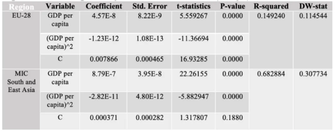
After seeing that the turning points for the two regions are statistically significantly different from one another, regression results using the FEM model for each region are conducted. The regression results can be seen in Table 4.

Table 4 Regression results (for eq. 1) using Least Squares Fixed Effect Model

From the regression results in Table 4, equation 4 and 5 are conducted.

(4) CO2EUt = 0.008209 + 4.55E-8(GDP per capita)EUt – 1.25E-12(GDP per capita)2EUt

(5) CO2ASIAt = 0.000529 + 8.78E-7 (GDP per capita)ASIAt – 2.82E-11(GDP per capita)2ASIAt

After generating the equations using the Fixed Effect Model for the EU and for MIC in South and East Asia, the turning point for the relationship between CO2 and economic

growth is calculated for each region. The turning points are calculated using Equation 2 (Dinda, 2004) and regression results from Table 4.

Turning point for the European Union using FEM:

T(FEM) = − 𝛽1/(2𝛽2 ) = - 4.55E-8 / (2*(-1.25E-12)) = 18 200

Turning point for Southern and Eastern middle income countries in Asia using FEM:

T(FEM) = − 𝛽1/(2𝛽2 ) = - 8.78E-7 / (2*(-2.82E-11)) = 15 567

Complementary to the statistical test when testing for a difference in turning points between the two regions, calculations are made to strengthen the results. As seen by the calculations, the turning point for the Asian economies is at a lower level of economic growth than for the European Union.

3.5.2 Second Hypothesis

There is a significant difference between the European Union and the South and East Asian middle income countries when comparing the decoupling process of economic growth and carbon emissions.

When testing for the second hypothesis, the average level of income is calculated for 2014 for each region. Thereafter, the individual slope coefficients will be calculated by taking the first derivative of the functions. If the slope coefficient is positive, relative decoupling is seen and if the slope is negative, absolute decoupling is present.

H0: 𝛽EU = 𝛽ASIA H1: 𝛽EU≠ 𝛽ASIA

Calculations for the European Union using FEM:

Average GDP per capita for year 2014: 34 567

CO2EUt = 0.008209 + 4.55E-8(GDP per capita)EUt – 1.25E-12(GDP Per capita)2EUt

Derivative of the slope in 2014 is calculated by the following function:

ΔCO2EUt = 4.55E-8 – 2.5E-12(GDP per capita)EUt

ΔCO2EU2014 = 4.55E-8 – 2.5E-12(34 567)EU2014 = -4.09175E-8

Slope coefficient < 0, which indicates absolute decoupling for the EU in 2014.

Calculations for the Asian countries using FEM:

Average GDP per capita for year 2014: 3 876

CO2ASIA2014 = 0.000529 + 8.78E-7 (GDP per capita)ASIA2014 – 2.82E-11(GDP per capita)2ASIA2014

Derivative of the slope in 2014 is calculated by the following function:

Δ CO2ASIAt = 8.78E-7 – 5.64E-11(GDP per capita)ASIAt

Δ CO2ASIA2014 = 8.79E-7 – 5.64E-11(3876)ASIA2014 = 6.59394E-7

Slope coefficient > 0, which indicates relative decoupling for the Asian region in 2014.

Since -4.09175E-8 ≠ 6.59394E-7, we reject the null hypothesis that the slopes for the two regions are equal. By comparing the slope coefficients for both regions above, it can be concluded that the null hypothesis is rejected. This means that there is a significant difference between the decoupling processes in the EU and South and East Asian middle income countries.

3.6 Robustness Check

In this section we conduct a robustness check of the Random Effect Model for both sets of panel data. As seen in Table 5, the coefficients for Fixed Effect Model used in the method are very similar to the coefficients for REM for both regions. To strengthen this statement, calculations for the turning points using REM for both regions are made. Thereafter, the differences between the turning points for each region using different models is calculated to see if there are large differences. Turning points are calculated using equation 2 (Dinda, 2004) and regression results from Table 5:

Calculations for the EU countries using REM:

T(REM) = − 𝛽1/(2𝛽2 ) = - 4.57E-8 / (2*(-1.23E-12)) = 18 577

ΔT = T(REM) - T(FEM) = 18 577- 18 200 = 377

Calculations for the Asian countries using REM:

T(REM) = − 𝛽1/(2𝛽2 ) = - 8.79E-7 / (2*(-2.82E-11)) = 15 585

ΔT = T(REM) - T(FEM) = 15 585 - 15 567 = 18

The results show that the difference between the turning points using REM and FEM are very small. Therefore, we use the FEM as our main model. This is done to make the statistical comparison possible.

Table 5 Regression results using Least Squared Random Effect Model (for eq. 1)

4. Discussion

To test for the first hypothesis, that there is a significant difference of the turning points between the European Union and South and East Asian middle income countries, the results indicated that there is a significant difference between the two regions. The results showed that the EU had a turning point higher than that of the Asian region, indicating differences between the two. Furthermore, to test the second hypothesis, the slope coefficient of 2014 was calculated for each region. The results showed that the alternative hypothesis was not rejected, implying that the decoupling processes of the two regions differ. It was found that the EU had decoupled in absolute terms in 2014, but the Asian region had only decoupled in relative terms. However, it is important to point out that these calculations might differ from similar studies as the results conducted in this study showed little evidence of cointegration and in turn a long run relationship between the variables. A reason for this potential problem is that there could be other variables explaining the relationship between environmental degradation and economic growth better, and that there is missing data for many of the countries for the earlier years of this study. However, since we found some evidence of cointegration and that we strengthen our results with previous studies investigating the relationship between the variables, an assumption that there is cointegration could be done to further analyze the results generated (Aye and Edoja, 2017). It is also important to point out that even if a long run relationship would have been found, the EKC is attributed to be sensitive to results from different data sources, therefore the results could differ from similar studies either way.

When comparing the results found in our study with previous empirical results, found in section 2.5, differences in the decoupling processes between the European countries and middle income countries in South and East Asia can be seen. According to Liobikienė and Dagiliūtė (2016) absolute decoupling was only seen in some of the EU countries between 1993 and 2010, whereas our results indicated that absolute decoupling can be seen throughout the entire EU when making a generalization of all countries. These results imply that in 2014, absolute decoupling was seen in the EU as a whole, however, there could still be differences between countries as the decoupling process at an individual level most likely differs. Similar to our results for the Asian region, Zhang et al., (2020) only found weak relative decoupling in ASEAN and China, which indicates that they are far from absolute decoupling.

The decoupling trends can be explained by the theories of Rostow's Stages of Growth and the Ecological Modernization theory. As suggested by Rostow (1999), an economy experiences different stages of economic growth and in turn environmental concern. A conclusion that can be drawn from the theory is that both Asia and the EU might have gone through similar stages as the theory suggests, however in different phases and at different points in time. The fourth stage, which is mass consumption, is a stage that the EU supposedly went through during the 1950’s (Rostow, 1999). Whereas when analyzing our results, the assumption that part of Asia went through the same phase at a later point in time can be drawn. When analyzing the results, it could be assumed that the EU is currently in stage five, indicating that people seek satisfaction in other forms than only through consumption. This could be a reason why they are currently facing absolute decoupling. In stage five, marginal utility of consumption starts to diminish and people seek satisfaction in new forms. This could be, for example, through caring for environmental changes and through innovation of technological methods that are in favor of the environment. It can also be discussed that the Asian countries have not yet reached this stage, since they are far from absolute decoupling. Currently relative decoupling is seen, however increased effects on technological changes will potentially reach the Asian countries sooner than it did for the EU, therefore absolute decoupling will be seen at a lower level of economic growth.

Similar to Rostow's stages of growth theory, the Ecological Modernization theory suggests that an economy experience different stages. The theory also suggests that a society and its concern about environmental degradation is dependent mostly on technological development. When a society has reached a certain stage of economic development the concern of environmental degradation is no longer solely dependent on top-down governance, but rather dependent on the voice of the people and its social aspects (Mol and Sonnenfeld, 2007). As most of the EU and the Asian countries considered in this study are currently experiencing similar stages of improvements in technological development, the estimated stagnation of the relationship between carbon emissions and economic growth could be explained partially by technological improvements and social effects. Despite experiencing economic growth at different levels and in different phases, currently global technology affects both Asia and the EU in similar matters. Even though the EU has a level of GDP far beyond that of the Asian countries, they are still able to reach much of the same information and environmental concern, which in turn might have affected their economic behavior and partially therefore, they will reach absolute decoupling at a lower level of economic growth than the EU.

One implications of this study, however, is that only CO2 is considered as a proxy for environmental degradation, this could be one of the reasons why cointegration between the variables is only seen in some tests. However, we support the relationship between the variables through previous studies (Dinda, 2004) (Mikayilovet al., 2018). The results will therefore only indicate decoupling of carbon emissions to economic growth and will not explain all greenhouse gasses. Another limitation is that the data is only available until 2014, more recent data could have given slightly different results as the EKC is sensitive to differences in data sources. It could also have indicated that the criticism of the EKC is valid. Newer data might have shown an N-shaped relation between the variables for the EU representing a potential increase in environmental degradation beyond a certain level of income. The reason for this potential increase in environmental degradation, is the decrease in effects of technological changes and the consistency of scale effects. The lack of recent data could also mean that the Asian countries might currently be closer to absolute decoupling, as much can happen in 5 years.

The last limitation taken into consideration concerns generalization of the two regions. Although most countries in each region have similar levels of economic growth, there are still many differences. These differences might indicate that the decoupling processes of the different countries in the regions might not be the same. Hence it is important to take into consideration that this is only a generalization of all countries in the entire EU and middle income countries in the Southern and Eastern Asia respectively. The results could also be biased to some extent since there is missing data for the earlier years for some countries. Another concern is that most EU countries are net importers of trade. One of the potential reasons why strong absolute decoupling is seen, is the EU offshoring much of their production to other countries, such as in Southeast Asia. This might be another potential reason why absolute decoupling is seen in the EU.

5. Conclusion

This paper is an evaluation of the decoupling processes of carbon emissions and economic growth in middle income countries in East and South Asia and the European Union, two regions currently experiencing different stages of economic growth. The results conducted in this study indicates that there are differences between the turning points of the relationship between CO2 and economic growth, and in turn the decoupling processes in the two regions differ when an assumption of correlation between the variables is made. When analyzing and comparing the trends of the relationship, we found that the EU had decoupled their economy in absolute terms in 2014. However, the Asian economies only showed signs of weak relative decoupling. These results could also be explained by the theories of Rostow's stages of growth and the Ecological Modernization theory indicating that economic behavior differs depending on what economic state a country is in.

Assuming that there is a long run relationship between the variables, this study compares two regions with very different economic development levels, regulations, policies and totally different perspectives when it comes to sustainability and environmental regulations. For this reason, an insight of how diversified and flexible policy makers should be when drafting programs for different regions can be seen. Our results together with the theories indicates that technology and social awareness is improving the process of reaching absolute decoupling at lower levels of GDP per capita.

This paper can contribute to future studies analyzing and criticizing the decoupling processes of different regions, as well as to investigate the decoupling process in individual countries rather than as a generalization of a region. With more data and more recent data, future studies might differ slightly from the results presented in this paper, which opened the possibility to further contribute to the discussion of the relationship between decoupling and theoretical studies. It could also contribute to further research dividing carbon emissions into categories. Since the EU countries are net importers of trade, investigating consumption based carbon emission would be interesting, considering the EU offshoring much of their production to other countries such as Southeast Asian countries. A reason for these changes in production locations could be explained by the EU protecting their reputation as forerunners within decoupling. This highlights the importance to develop international policies to strengthen the decoupling process worldwide.

6. Reference list

Allard, A., Takman, J., Uddin, G., & Ahmed, A., (2017). The N-shaped environmental Kuznets curve: an empirical evaluation using a panel quantile regression approach.

Environmental Science And Pollution Research, 25(6), 5848-

5861. https://doi.org/10.1007/s11356-017-0907-0

Alvarez-Herranz, A., Balsalobre-Lorente, D., Shahbaz, M., & Cantos, J., (2017). Energy innovation and renewable energy consumption in the correction of air pollution levels. Energy Policy, 105, 386-397. https://doi.org/10.1016/j.enpol.2017.03.009

Aye, G., & Edoja, P., (2017). Effect of economic growth on CO2 emission in developing countries: Evidence from a dynamic panel threshold model. Cogent Economics &

Finance, 5(1). https://doi.org/10.1080/23322039.2017.1379239

Baltagi, B. (2010). Fixed Effects and Random Effects. Microeconometrics, pp. 59-64.

Breusch, T. & Pagan, A., (1980). The Lagrange Multiplier Test and its Applications to Model Specification in Econometrics. The Review of Economic Studies, 47(1), p.239. https://doi.org/10.2307/2297111

Buttel, F., (2000). Ecological modernization as social theory. Geoforum, 31(1), 5765. https://doi.org/10.1016/S0016-7185(99)00044-5

CO₂ emissions embedded in trade. (2020). [online] Available at: https://ourworldindata.org/grapher/co-emissions-in-imported-goods-as-a-shareof-domestic-

emissions?tab=chart&country=KHM+IND+IDN+KAZ+KWT+KGZ+LAO+M YS+PAK+PHL+LKA+THA+VNM [Accessed 11 May 2020]

Conrad, E., & Cassar, L., (2014). Decoupling Economic Growth and Environmental Degradation: Reviewing Progress to Date in the Small Island State of Malta.

Sustainability, 6(10), 6729-6750. https://doi.org/10.3390/su6106729

Datahelpdesk.worldbank.org. (2020). How Does The World Bank Classify Countries? – World Bank Data Help Desk. [online] Available at:

https://datahelpdesk.worldbank.org/knowledgebase/articles/378834-how-doesthe- world-bank-classify-countries [Accessed 11 May 2020].

Dinda, S., (2004). Environmental Kuznets Curve Hypothesis: A Survey. Ecological Economics, 49(4), 431-455. https://doi.org/10.1016/j.ecolecon.2004.02.011

European Commission, (2018). EU on track to implement Paris commitments, Member States preparing 2030 energy and climate plans - Climate Action - European Commission [online] Available at:

https://ec.europa.eu/clima/news/eu- trackimplement-paris-commitments-member-states-preparing-2030-energy-and-climateplans_en [Accessed 13 February 2020]

Granger, C. & Newbold, P., (1974). Spurious regressions in econometrics. Journal of

Econometrics, 2(2), 111-120. https://doi.org/10.1016/0304-4076(74)90034-7

Hausman, J. (1978). Specification Tests in Econometrics. Econometrica, 46(6), 12-51. doi: 10.2307/1913827

Hurley, J., Storrie, D., & Peruffo, E. (2016). ERM annual report 2016: Globalisation slowdown? Recent evidence of offshoring and reshoring in Europe. Luxembourg: Publications Office of the European Union. [online] Available at: http://publications.europa.eu/resource/cellar/ecc4031a-e921-11e6-ad7c-

01aa75ed71a1.0001.02/DOC_2 [Accessed 12 March]

Im KS, Pesaran MH., & Shin Y., (2003) Testing for unit roots in heterogeneous panels.

Journal of Econometrics; 115: 53–74. https://doi.org/10.1016/S0304-4076(03)00092-7

Intergovernmental Panel on Climate Change. (2006). IPCC National Greenhouse Gas

Inventories Programme. [online] Available at:

https://www.ipccnggip.iges.or.jp/support/Primer_2006GLs.pdf [Accessed 15 March 2020]

IRP (2017). Assessing global resource use: A systems approach to resource efficiency and pollution reduction. Bringezu, S., Ramaswami, A., Schandl, H., O’Brien, M., Pelton, R., Acquatella, J., Ayuk, E., Chiu, A., Flanegin, R., Fry, J., Giljum, S., Hashimoto, S., Hellweg, S., Hosking, K., Hu, Y., Lenzen, M., Lieber, M., Lutter, S., Miatto, A., Singh Nagpure, A., & Kuroda, Y. (1989). Impacts of economies of scale and technological change on agricultural productivity in Japan. Journal Of The Japanese And International

Economies, 3(2), 145-173.

Levin, A., Lin, C. & James Chu, C., (2002). Unit root tests in panel data: asymptotic and finite-sample properties. Journal of Econometrics, 108(1),1-

24. https://doi.org/10.1016/S0304-4076(01)00098-7

Liobikienė, G., & Dagiliūtė, R., (2016). The relationship between economic and carbon footprint changes in EU: The achievements of the EU sustainable consumption and production policy implementation. Environmental Science & Policy, 61, 204211. https://doi.org/10.1016/j.envsci.2016.04.017

Lorente, D., & Álvarez-Herranz, A., (2016). Economic growth and energy regulation in the environmental Kuznets curve. US National Library Of Medicine National Institute Of

Health, 23(16), 16478-16494. https://doi.org/10.1007/s11356-016-6773-3

Ma, X., Ye, Y., Shi, X., & Zou, L., (2016). Decoupling economic growth from CO2 emissions: A decomposition analysis of China's household energy consumption.

Advances In Climate Change Research, 7(3), 192- 200. https://doi.org/10.1016/j.accre.2016.09.004

Mikayilov, J., Hasanov, F., & Galeotti, M., (2018). Decoupling of CO2 emissions and GDP: A time-varying cointegration approach. Ecological Indicators, 95, 615628. https://doi.org/10.1016/j.ecolind.2018.07.051

Ming, Z., Ximei, L., Yulong, L., & Lilin, P., (2014). Review of renewable energy investment and financing in China: Status, mode, issues and countermeasures. Renewable And

Sustainable Energy Reviews, 31, 23-37. https://doi.org/10.1016/j.rser.2013.11.026

Mishra, V., (1995). A Conceptual Framework for Population and Environment Research. Laxenburg: International Institute for Applied Systems Analysis. [online] Available at: http://pure.iiasa.ac.at/id/eprint/4572/1/WP-95-020.pdf [Accessed 3 April]

Mol, A., & Sonnenfeld, D., (2007). Ecological modernisation around the world: An introduction. Environmental Policies, 9(1), 1-14. doi: 10.1080/09644010008414510

Mulvaney, K., (2019). Climate change report card: These countries are reaching targets. 2020

[online] Available at:

https://www.nationalgeographic.com/environment/2019/09/climate-changereport-card-co2-emissions/ [Accessed 11 February]

National Inventory Submissions 2018. (2020). [online] Available at: https://unfccc.int/process-and-meetings/transparency-and-reporting/reportingand-review-under-the-convention/greenhouse-gas-inventories-annex-i-

parties/submissions/national-inventory-submissions-2018 [Accessed 21 February 2020]

Panayotou, T., (1993). Empirical Tests and Policy Analysis of Environmental Degradation at Different Stages of Economic Development.

Pedroni P. (1999). Critical values for cointegration tests in heterogeneous panels with multiple regressors. Oxf Bull Econ Stat; 61, 653–670. https://doi.org/10.1111/14680084.0610s1653

Renewable Energy Outlook for ASEAN. (2020). [online] Available at:

https://www.irena.org/publications/2016/Oct/Renewable-Energy-Outlook-forASEAN [Accessed 11 May 2020]

Rostow, W., (1999). The stages of economic growth (3rd ed., pp. 4-16). Cambridge [England]: Cambridge University Press.

Sanyé-Mengual, E., Secchi, M., Corrado, S., Beylot, A., & Sala, S., (2019). Assessing the decoupling of economic growth from environmental impacts in the European

Union: A consumption-based approach. Journal Of Cleaner Production, 236, 117535. https://doi.org/10.1016/j.jclepro.2019.07.010

Traivivatana, S., Wangjiraniran, W., Junlakarn, S., & Wansophark, N., (2017). Thailand Energy Outlook for the Thailand Integrated Energy Blueprint (TIEB). Energy

Procedia, 138, 399-404. https://doi.org/10.1016/j.egypro.2018.11.213

World Bank. (2020). [online] Available at:

https://www.worldbank.org/en/country/thailand/overview [Accessed 12 May 2020]

World Bank. (2020) [online] Available at:

https://data.worldbank.org/indicator/NY.GDP.MKTP.CD?locations=8S [Accessed 10 May 2020]

World Bank. (2020) [online] Available at:

https://data.worldbank.org/indicator/NY.GDP.MKTP.CD?locations=EU&name _desc=true [Accessed 11 May 2020]

World Bank. (2020) [online] Available at:

https://data.worldbank.org/indicator/NY.GDP.MKTP.CD?locations=Z4 [Accessed 13 May 2020]

Zhang, J., Fan, Z., Chen, Y., Gao, J., & Liu, W., (2020). Decomposition and decoupling analysis of carbon dioxide emissions from economic growth in the context of China and the ASEAN countries. Science Of The Total Environment, 714, 136649. https://doi.org/10.1016/j.scitotenv.2020.136649

Zhao, X., Zhang, X., Li, N., Shao, S., & Geng, Y., (2017). Decoupling economic growth from carbon dioxide emissions in China: A sectoral factor decomposition analysis.

Journal Of Cleaner Production, 142,. 3500-

3516. https://doi.org/10.1016/j.jclepro.2016.10.117

7. Appendix

7.1 Tables and graphs

Appendix 7.1.1 shows a list of all countries included in this study

Appendix 7.1.2 shows the Environmental Kuznets Curve

Source: Panayotou (1993)

Appendix 7.1.3 represents the N-shaped Environmental Kuznets curve

Source: (Alvarez et al., 2017)

7.2 Outputs from EViews

Appendix 7.2.1 represents the results of the Panel Unit Root Tests

Appendix 7.2.2 represents the Residual Cointegration Test

Appendix 7.2.3 represents the results of the Lagrange Multiplier Tests for Random Effects

Appendix 7.2.4 represents the results of the Hausman Test for Fixed Effect Model

Appendix 7.2.5 represents the result from an Cross-section correlation test

As seen from Appendix 7.2.5, it can be concluded that there is no problem with cross-section correlation for any of the two regions at a 1 % significance level, since all p-values are equal to 0.0000.