Fixed effects estimation of marginal railway infrastructure costs in Sweden

(1)

Fixed Effects Estimation of Marginal Railway Infrastructure

Costs in Sweden

(2)

Abstract

New railway legislation in Sweden has increased the need for transparent access charges on the Swedish railway network. We estimate cost functions for infrastructure operation, maintenance and renewal in the Swedish national railway network, using unobserved effects models and calculate marginal costs for railway infrastructure wear and tear. We find evidence of unobserved fixed effects at a track section level for infrastructure operation and maintenance costs. The estimated weighted average marginal infrastructure operation cost is SEK 0.12 per train kilometre and the estimated marginal maintenance cost is SEK 0.0073 per gross tonne kilometre. Altogether, the results indicate that the current charge for railway infrastructure wear and tear in Sweden is below marginal cost.

Keywords: Railway; Infrastructure operation; Maintenance; Renewal; Marginal costs; Fixed effects

(3)

1. Introduction

Sweden has new railway legislation since July 2004 (Riksdagen, 2004). This forces the Swedish National Rail Administration (Banverket) to set transparent fees for track access based on marginal social cost estimates in line with Swedish transport policy. The most important component today is the fee for infrastructure wear and tear, exceeding 60 percent of total access fees paid by train operating companies in recent years (Banverket, 2007). The current charge for infrastructure wear and tear is SEK 0.0029 per gross ton kilometre (Banverket, 2006)1.

Estimating cost functions for railway organisations has a long tradition, but early work use firm level time series and focuses on issues like productivity, economies of scale, scope and density, and capacity utilisation in the US freight market (Griliches, 1972; Keeler, 1974; Brown et al., 1979; Caves et al., 1980). More recent work includes Bereskin (2000) who estimates maintenance-of-way costs for US freight railways, and Bitzan (2003) who addresses the issue of cost effects from on-track competition in the US. To our knowledge, there are no published cost studies involving micro-level data from individual US railway organisations.

The use of micro-level data and the issue of marginal cost estimation have instead been a European affair. The problem has received increased attention in vertically separated rail sectors with multiple operating companies, in need of a non-discriminatory pricing regime. Pricing at marginal social cost is suggested from economic theory in order to optimally utilise the existing network. Swedish transport policy has marginal cost pricing as one of its

cornerstones and the recent government bill on transport (Regeringen, 2006) maintains this position. The Swedish government also emphasises the need for detailed estimates of marginal social costs in the Swedish railway sector.

1

The exchange rate from Swedish Kronor (SEK) to Euro (EUR) is SEK 9.23/EUR and from Swedish Kronor to US Dollar (USD) is SEK 6.78/USD (April 25, 2007).

(4)

Nash (2005) reviews the European situation and lists only a few empirical studies undertaken, with the majority never published in scientific journals. Nash also points out that Scandinavian countries are aiming at charging for marginal costs but most likely fall short of this due to a failure to charge for marginal renewal costs. This is also confirmed in a similar review of railway infrastructure pricing by Link and Nilsson (2005).

In fact, the only published studies using micro-level data to date are Swedish studies. Johansson and Nilsson (2004) apply a Translog cost function specification (Berndt and Christensen, 1973) on railway track section data covering Sweden in 1994-1996 and Finland in 1997-1999. The final model for Sweden uses a pooled data set with infrastructure

maintenance costs as dependent variable. For Finland, the data also includes renewal costs. The cost elasticity with respect to output (track section gross tonnes per year) in both Sweden and Finland is estimated to 0.17. The main result is marginal costs estimates of track wear and tear related to traffic for each country. The overall estimates are SEK 0.0012 for Sweden and SEK 0.0023 for Finland per gross tonne kilometre.

Andersson (2006) applies pooled ordinary least squares (POLS) to a panel of Swedish data over the years 1999-2002, with track section information on costs, traffic and

infrastructure. He finds that a separation of infrastructure operation costs, mainly snow removal, from maintenance and renewal costs is warranted as the former is driven by trains and the latter two by gross tonnes. The infrastructure operation cost elasticity with respect to traffic is estimated to 0.37, and marginal cost SEK 0.48 per train kilometre. The average maintenance cost elasticity is estimated to 0.21, and marginal cost SEK 0.0031 per gross tonne kilometre. The final model estimates are based on an aggregate of maintenance and renewal costs with an average elasticity with respect to traffic of 0.26 and marginal cost at SEK 0.0055 per gross tonne kilometre.

(5)

In this paper we extend the work in Andersson (2006) and estimate cost functions for infrastructure operation, maintenance and renewal in the Swedish national railway network as well as derive marginal costs based on estimated relationships. Specifically, the purpose of the paper is to use panel data econometric techniques in order to assess the possible significance of having unobserved effects driving the cost structure and to avoid omitted variable bias.

The outline of this paper is the following. Section 2 gives an overview of the available data. A variety of econometric modelling issues are discussed in section 3. Section 4 is devoted to the results from the econometric models. In section 5, we present marginal cost calculations from our estimated models and section 6 concludes.

2. Swedish Railway Network Data

Cost data on infrastructure operation, maintenance and renewal is available for roughly 185 track sections per year from 1999 to 2002 (table 1). Our focus in this analysis is

completely on infrastructure costs; hence no costs for running train services are included in our analyses. Infrastructure operation is dominated by snow removal (80 %). Activities in this cost group have a very short time horizon and are undertaken to keep the track open for train movements. Maintenance activities have a somewhat longer time horizon and are in most cases needed at least once biannually in order to prevent the track from premature

degradation. Tamping, ballast cleaning and switch overhaul fall into this category. Finally, renewal activities have a longer time horizon and are undertaken every 20-60 years. A renewal is an activity aiming at bringing the track back to its original condition. Rail and switch replacements are examples of renewal activities.

There is some variation in average costs per track section over the years of observation for all three different activities and variation is also substantial between track sections. We

(6)

can also observe renewal costs being skewed to the right from the fact that all track sections do not experience renewal activities every year.

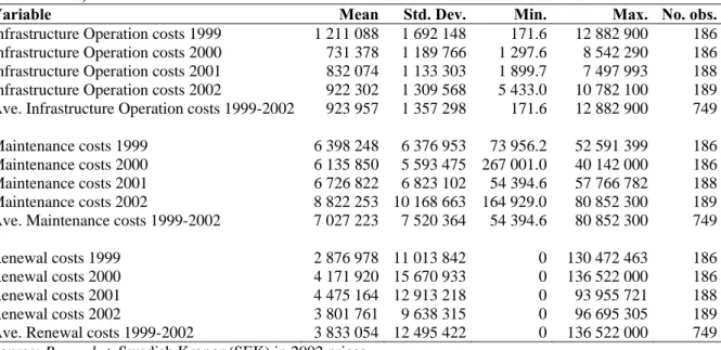
TABLE 1. Costs for infrastructure operation, maintenance and renewal per track section (1999-2002).

Variable Mean Std. Dev. Min. Max. No. obs.

Infrastructure Operation costs 1999 1 211 088 1 692 148 171.6 12 882 900 186

Ave. Infrastructure Operation costs 1999-2002 923 957 1 357 298 171.6 12 882 900 749

Maintenance costs 1999 6 398 248 6 376 953 73 956.2 52 591 399 186

Ave. Maintenance costs 1999-2002 7 027 223 7 520 364 54 394.6 80 852 300 749

Renewal costs 1999 2 876 978 11 013 842 0 130 472 463 186

Renewal costs 2000 4 171 920 15 670 933 0 136 522 000 186

Renewal costs 2001 4 475 164 12 913 218 0 93 955 721 188

Renewal costs 2002 3 801 761 9 638 315 0 96 695 305 189

Ave. Renewal costs 1999-2002 3 833 054 12 495 422 0 136 522 000 749

Source: Banverket. Swedish Kronor (SEK) in 2002 prices.

There is also a wide range of technical features of the railway track summarised in table 2 that can be expected to influence costs in either a positive or negative way. These were examined as covariates in the cost functions estimated by Andersson (2006). It should however be noted that the majority of the variables show very little or no variation over time at a track section level and are highly correlated with each other, which normally give rise to multicollinearity problems in the model estimation phase. Some of these variables also have missing data in the original data set and single imputation techniques have been used to complete the data set (see Andersson (2006) for details).

Finally, we have a selection of traffic variables that can be used as a measure of output from the track (table 3). We have access to information on gross tonnes and trains for

passenger as well as freight transport over the four years. Combined with information on track distance, we get traffic expressed as gross ton kilometres and train kilometres. Dividing

(7)

tonnage by trains gives us an average train weight per track section, for total traffic, and per freight and passenger train. Some track sections have no passenger services so average weight is not computable for these observations; hence the two rows with and without zero

observations.

TABLE 2. Infrastructure data per track section, 1999-2002

Variable Mean Std. Dev. Min. Max. No. obs.

Track section distance (i) 51 500.8 42 994.4 1 500.0 213 600.0 749

Track section length (i) 71 136.5 54 395.3 3 719.0 261 561.0 749

Tunnels (i) 318.4 1 299.6 0.0 13 799.1 749

Bridges (i) 577.9 989.1 0.0 9 412.7 749

Rail weight (ii) 50.1 5.1 32.0 60.0 749

Rail gradient (i) 50 144.7 44 766.7 0.0 261 602.0 749

Rail cant (i) 27 865.8 26 144.4 0.0 136 799.0 749

Curvature (i) 15 082.8 14 000.4 0.0 89 561.9 749

Lubrication (iii) 10.9 19.3 0.0 115.0 749

Joints (iii) 155.4 131.3 0.0 799.0 749

Continuous welded rails (i) 49 181.5 52 607.4 0.0 286 400.0 749

Frost protection (i) 3 535.2 10 098.9 0.0 69 250.0 749

Switches* (i) 1 687.8 1 721.4 58.0 14 405.0 749

Switch age* (iv) 18.8 9.7 1.0 68.0 749

Sleeper age* (iv) 18.3 13.1 1.0 98.0 749

Rail age* (iv) 18.7 12.9 1.0 98.0 749

Ballast age* (iv) 19.4 13.5 1.0 98.0 749

Track quality class* (v) 2.3 1.1 0.0 4.9 749

Source: Banverket, Track Information System (BIS). (i) - Track meters; (ii) – Kilograms per meter; (iii) – Number of; (iv) - Years; (v) - Index 0 (high) – 5 (low); * Missing data in original data set.

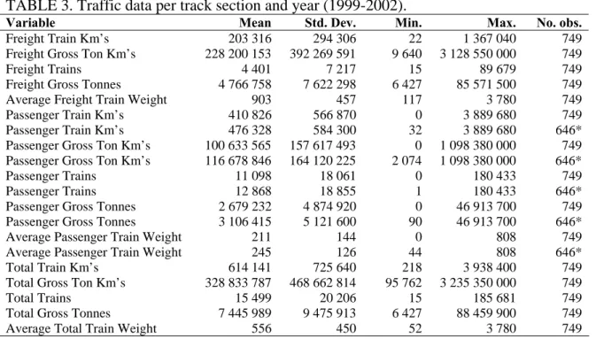
TABLE 3. Traffic data per track section and year (1999-2002).

Variable Mean Std. Dev. Min. Max. No. obs.

Freight Train Km’s 203 316 294 306 22 1 367 040 749

Freight Gross Ton Km’s 228 200 153 392 269 591 9 640 3 128 550 000 749

Freight Trains 4 401 7 217 15 89 679 749

Freight Gross Tonnes 4 766 758 7 622 298 6 427 85 571 500 749

Average Freight Train Weight 903 457 117 3 780 749

Passenger Train Km’s 410 826 566 870 0 3 889 680 749

Passenger Train Km’s 476 328 584 300 32 3 889 680 646*

Passenger Gross Ton Km’s 100 633 565 157 617 493 0 1 098 380 000 749

Passenger Gross Ton Km’s 116 678 846 164 120 225 2 074 1 098 380 000 646*

Passenger Trains 11 098 18 061 0 180 433 749

Passenger Trains 12 868 18 855 1 180 433 646*

Passenger Gross Tonnes 2 679 232 4 874 920 0 46 913 700 749

Passenger Gross Tonnes 3 106 415 5 121 600 90 46 913 700 646*

Average Passenger Train Weight 211 144 0 808 749

Average Passenger Train Weight 245 126 44 808 646*

Total Train Km’s 614 141 725 640 218 3 938 400 749

Total Gross Ton Km’s 328 833 787 468 662 814 95 762 3 235 350 000 749

Total Trains 15 499 20 206 15 185 681 749

Total Gross Tonnes 7 445 989 9 475 913 6 427 88 459 900 749

Average Total Train Weight 556 450 52 3 780 749

(8)

3. Modelling issues

Selecting the right model for the purpose of estimating marginal costs of infrastructure wear and tear is not straightforward. Decisions have to be made about which estimation technique to use, the choice of dependent variable and the independent variables considering both observed and unobserved data. In the following sections, we will discuss these issues in the light of the available data.

3.1. Econometric estimation techniques

The fact that we have a combination of cross-section (track sections) and time-series (observed over four years) data gives us the option to use so called panel data models (also known as unobserved effects models). An alternative is instead to pool the entire data set as in Johansson and Nilsson (2004) and Andersson (2006), and treat it as a large cross-section sample and estimate one model per cost category based on all 749 observations using OLS.

The most basic forms of panel data models can be grouped into fixed effects (FE) and random effects (RE). This will serve as a starting point for our discussion and model

selection. Still, we acknowledge that panel data econometrics are by far more complex and diverse than just choosing between FE and RE models (see Wooldridge (2002) or Baltagi (2005) for a more thorough coverage of the field).

Greene (2003) uses regression model (1) as a baseline for a discussion of the differences between POLS, FE and RE.

T t N i y_it =x_it′β+z_i′α+ε_it, =1,2,..., =1,2,..., (1) it

y is our dependent variable, is a vector containing K observed variables on N observations over T periods that can vary in both the i (individual) and t (time) dimensions.

it

(9)

Models exploring variation only in the i-dimension are commonly named one-way models while models exploring variation in both i and t-dimensions are known as two-way models. Heterogeneity in the data is captured in z_i′ , which includes a constant term and a set of α individual or group specific observations, observed or unobserved. α and β are vectors of parameters to be estimated and ε_it is the error term.

A pooled regression (2) is simply when contains only a column of ones to capture a common constant term α and OLS will then give consistent and efficient estimates of

i z α and . β T t N i yit =xit′β+α +εit, =1,2,..., =1,2,..., (2)

The FE model emerges when in (1) contains an unobserved effect that is correlated with . OLS will then give biased and inconsistent estimates due to omitted variables if expression (2) is used. Using an individual specific constant,

i z it x i α , as in expression (3), will on

the other hand give both unbiased and consistent estimates of all model parameters.

T t

N i

yit =αi +x′itβ+εit, =1,2,..., =1,2,..., (3)

A well known feature of the FE estimator is that it requires a large number of parameters to be estimated, which consumes degrees of freedom when there are a large number of individual effects to account for. The RE model does not come with this feature as it (like POLS) only estimates a common constant α along with the coefficient vector β. It is also possible to add time-invariant individual features to this model. Expression (4) gives the RE model.

(10)

T t N i u y_it =x_it′β+α + _i +ε_it, =1,2,..., =1,2,..., (4)

The RE approach specifies to be an individual specific random element. The crucial assumption is that the unobserved heterogeneity needs to be uncorrelated with the included variables in . The model can be consistently, but inefficiently estimated by OLS. Efficient estimation is done by Feasible Generalised Least Squares (FGLS), accounting for within- and between-group correlation of the error term. If the assumption that the unobserved

heterogeneity is uncorrelated with does not hold, RE estimation is inconsistent.

i u it x it x

The fundamental advantage of keeping the data in the panel format is that it will allow us to model individual differences between our included track sections if we assume that such heterogeneity exist (Greene, 2003). In practitioners’ circles, track sections are often viewed as non-comparable entities that need to be treated individually. If the unobserved effects are constant over time, a fixed or random effects model would account for this feature and allow us to estimate models based on a sample of track sections. The group specific effects can either be modelled as track section constants or track section specific random elements. Wooldridge (2002) also emphasises the benefit of eliminating omitted variable bias as an argument for unobserved effects models.

3.2. The choice of dependent variable

Both infrastructure operation and maintenance are known as recurring activities and have a relatively short life span as described in section 2. Annual observations on costs for these activities are therefore quite straightforward to use in an econometric specification, where potential explanatory variables are observed on an annual basis.

(11)

Renewals are somewhat different and can be seen as rare events. The probability that we will observe a renewal at a specific track section is less than unity and we can see from table 1 that there are track sections each year where no renewals have been undertaken. A comprehensive time series of renewal costs on each track section is not available to us so we cannot calculate an overall life-cycle cost for renewals per track section.

Trying to explain renewal costs using a traditional regression model can look somewhat troublesome when we can expect renewal decisions being based on information gathered over a longer period of time than just one year. Johansson and Nilsson (2004) experienced this problem with Finnish data where information about renewal costs was available.

Andersson (2006) however did not observe this problem, which indicates that

maintenance and renewal decisions in Sweden are based on the same information within the same planning framework. This has also been confirmed in discussions with representatives of Banverket. Banverket receives funds for operation and maintenance separate from renewal, but the borderline between maintenance and renewal is not clear cut. It seems possible to categorise an activity as one or the other, making a strict separation of the two less motivated. We will therefore try and model the aggregate of maintenance and renewal as previously done in Andersson (2006).

3.3. Observed effects

Table 2 and 3 summarise our knowledge about the railway track and its use. We will initially discuss how to deal with the available infrastructure variables and then take a closer look at our traffic (or output) variables.

(12)

3.3.1. The choice of independent infrastructure variables

A railway network is a combination of various technical components. At a given level of output, we expect the infrastructure variables in table 2 to have a positive or negative effect on the cost level. We could go through each of the infrastructure variables to establish our a priori expectations, but all that we are genuinely interested in is the relationship between traffic and costs while controlling for individual features. The fact that we have a short observation period for our panel gives little or no variation in our observed infrastructure variables. We will therefore model infrastructure as a time-invariant unobserved effect. The only infrastructure covariate that we will include is rail age as it by nature is non-constant over time. It will be used as a proxy for all age variables as these are highly correlated. Our hypothesis is that age has a positive relationship with maintenance and renewal costs.

A well known feature of a railway network is that it is highly regulated in several dimensions. Rules and regulations exist for construction, renewal, inspections, proactive and reactive maintenance as well as the dispatching of trains. Even if we a priori easily can identify a number of factors that we expect to affect costs in a certain way, the actual joint modelling of all these variables will most likely give rise to problems of multicollinearity as found in Andersson (2006). Around 75 – 80 percent of the cost variation was explained with only a few of the listed infrastructure variables included in the estimated POLS models. There is little guidance available from theory in this case on which variables to use and including all variables, we might overfit the model. This problem is solved if we use unobserved effects models and group all time-invariant features into a track section constant or random element.

3.3.2. The choice of independent output variables

The range of variables in table 3 opens up for a number of possible model specifications and analyses, where output from the track can be expressed in different ways. We measure

(13)

output from the track in terms of traffic volume per year. In this paper we will restrict ourselves to the selection of total output variables, where freight and passenger trains are aggregated. We then follow the idea that a train is a train and a gross tonne is a gross tonne, whether it is passenger or freight. The issue of differentiation between these modes is an important one, especially from a differentiated pricing point of view. This question will therefore be covered in subsequent work. Furthermore, we like to model track length

independently from output. In such a case, we should use trains rather than train kilometres in our model specification to fully identify this effect. Similarly, we should use gross tonnes instead of gross tonne kilometres.

The Swedish railway legislation specifies that prices shall reflect utilisation (Riksdagen, 2004) and it is of great importance to make reasonable assumptions on which output to use in our models. With infrastructure operation costs being dominated by snow removal, we expect this group to have a stronger link to trains than gross tonnes. The weight of a train is unlikely to influence the need for snow removal, but the train itself will. Maintenance and renewal activities on the other hand are more likely to be driven by train loads, in our case represented by gross tonnes. Previous work on Swedish data by Johansson and Nilsson (2004) used aggregate costs on infrastructure operation and maintenance, but Andersson (2006) argued for a separation of these two groups, mainly from an output perspective. It was also shown that cost separation and use of different output variables are possible from an econometric point of view.

3.4. Unobserved effects

Apart from modelling our observed infrastructure variables as unobserved effects, there may be other factors that can have a strong impact on the cost for operation, maintenance and renewal. Firstly, we have not got a complete view of the infrastructure for each track section.

(14)

Secondly, the track sections are geographically spread from south to north and experience strong climate differences. Even between adjacent track sections, these differences can be substantial. Climate differences will be captured as an unobserved effect. Thirdly, the track district manager has the freedom of choice in spending an allocated budget within the safety rules and regulations of Banverket. Managerial skills and approaches will differ between districts and sections.

3.5. Modelling assumptions and approach

Estimating cost functions rely on the duality between cost and production functions. We will assume that Banverket acts as a cost minimising agency with respect to output, prices and technological features and that the costs we observe are results of cost minimising behaviour. Kennedy and Smith (2004) investigated the productivity and efficiency of Railtrack in the UK and found some potential for efficiency improvements, which might question this assumption. Still, this conclusion is, as always, based on information available for the study and Kennedy and Smith acknowledge that there might be other unobserved factors that could affect their standpoint. We will therefore maintain the assumption of cost minimisation in our study.

Another assumption is related to variation in quality over time. We assume that the quality of the track, on an individual track section, is maintained in such a way that it is held constant over the study period and included in the unobserved effect. An ideal solution would include track geometry measurements, but these are unavailable to us.

Based on the discussion above, we will take the following approach in our estimations. Operation costs will be modelled separately. Maintenance, on the other hand, will be dealt with both separately and combined with renewals.

We will assume a Translog production function and explore and include higher order terms when significant. The Translog specification was introduced to railway cost analysis by

(15)

Brown et al. (1979) and is a flexible form for estimating a cost function with an underlying functional form. The disadvantage of the Translog is the number of coefficients that have to be estimated, which drives the need for a large data set. Following the arguments by

Johansson and Nilsson (2004) against the inclusion of factor prices, we will also ignore price effects. The reason put forward in favour of excluding factor prices is the harmonisation of prices through a highly regulated labour market. Track sections are assumed to have a similar price structure when compared to each other. Another argument is that during this period, maintenance was in principal an in-house activity. The first trials towards competitive tendering of track section maintenance were done during 2002, the last year of our time window.

4. Econometric specifications and results

The outline of this section is that we first present the results from estimated models using infrastructure operation costs as dependent variable followed by maintenance costs only and finally an aggregate of maintenance and renewal costs. Stata 9 is used for all estimations (StataCorp, 2005).

4.1 A fixed effects specification for infrastructure operation costs

We have estimated a FE model (6) for the natural logarithm of infrastructure operation costs (lnCO), with unobserved effects assumed at the track section level. Included covariates are a third-degree polynomial of the natural logarithm of total number of trains (lnTT) as output. ε is a homoscedastic residual with zero mean, uncorrelated with the fixed effect and included covariates. The results are given in table 4. A scatter plot of residuals versus total trains indicates heteroscedasticity, and we therefore estimate the model with robust standard errors.

(16)

it it it it i O it TT TT TT C =α +β₁⋅ln +β₂⋅(ln )2 +β₃⋅(ln )3+ε ln (6)

Table 4. Results from a FE model for infrastructure operation costs

Variable Coefficient (Robust S.E.)

ln TT 5.916991† (2.300732)

(ln TT)2 -0.965014‡ (0.303143)

(ln TT)3 0.046071‡ (0.013062)

Number of observations = 749 Number of groups = 190

F(3, 556) = 5.63 Prob > F = 0.0008

Breusch-Pagan LM Test for Random Effects: χ2

(1)= 695.99 Correlation between unobserved

effect and included covariates = -0.60

σα = 1.819 σε = 0.636 ρ = 0.89

Legend: ‡ Significant at 1% level; † Significant at 5% level; * Significant at 10% level.

All coefficients are significant at the 1 percent level. The importance of the unobserved effect ui can be measured as (Wooldridge, 2002) with ρ in our model being 0.89. Almost 90 percent of the variation is contributed to the variation in our unobserved effect. The F-test shows that our model is significant at the 5 % level.

) /( 2 2 2 ε α α σ σ σ ρ = +

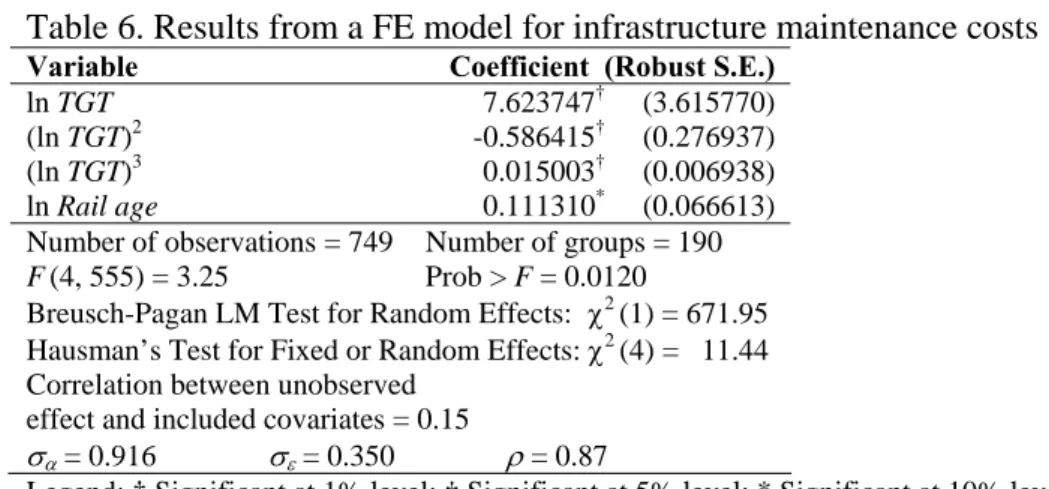
A well-known feature of the log-linear model is that estimated coefficients can be interpreted as elasticities (Gujarati, 1995). The standard way of deriving the output elasticity from a log-linear model is simply to take the derivative of the estimated cost function with respect to output. As we have specified a model using a third-degree polynomial for the natural logarithm of output we get a non-constant expression for the output elasticity (7).

O it it it O it _TT _TT TT C _β _β _β _γ ˆ ) (ln ˆ 3 ln ˆ 2 ˆ ln ln ₂ 3 2 1+ ⋅ ⋅ + ⋅ ⋅ = = ∂ ∂ (7)

Evaluating the cost function at lnTT and lnTT2 for each track section gives individual elasticities, and taking the mean results in an elasticity of -0.014. Thus, a one percent increase in output will give a -0.014 percent reduction in costs. This might look problematic at a first

(17)

glance, but a more detailed analysis of the elasticities show that they range from -0.81 to 2.8 (figure 1) and change from negative to positive as train volumes increase, at a decreasing rate. This confirms a view put forward by track managers at Banverket that train passages

contribute positively to snow removal by sweeping the snow off the track. We find that this effect is present up to annual volumes of around 12 000 trains or 32 trains per day. After that, we find increasing costs with increased train passages. A plausible explanation is that this comes from reduced track access times as well as higher demands on snow removal and de-icing as a standstill has larger negative effects on the rail system as a whole.

Figure 1: Infrastructure operation cost elasticities

-1 0 1 2 3 C o s t el as ti c it y 0 50000 100000 150000 200000

Total number of trains per year

Breusch and Pagan’s (1980) Lagrange Multiplier (LM) test is devised to test for zero correlation in the group-specific error terms, i.e. a test for a random effects model against the linear POLS model with a single constant term. Under the null hypothesis, the LM statistic is χ2

distributed with 1 degree of freedom. We get a test statistic value of 695.99, thus we can reject the null hypothesis at the 5 % level and conclude that a RE model is preferred to POLS.

The second step is that we also have to test for a selection between the FE and the RE specification. Hausman (1978) designed a test for orthogonality between the regressor and the random effect (Greene, 2003). Under the null hypothesis, the difference between the estimates

(18)

from the FE and RE models should not differ systematically. The FE estimator is consistent under both the null and alternative hypothesis, while the RE estimator is efficient under the null, but inconsistent under the alternative. Our decision criterion is then to stick with the RE model if our null hypothesis is maintained or the FE estimator if we reject the null hypothesis.

Table 5. Hausman’s specification test for fixed or random effects Variable Fixed effects

coefficients (b) Random effects coefficients (B) (b-B)

lnTT 5.916991 4.485870 1.431121

(lnTT)2 -0.965014 -0.555621 -0.409393

(lnTT)3 0.046071 0.023351 0.022720

Hausman’s test statistic: χ2

(3) = 22.76 Prob. > χ2

= 0.0000

The value of the test statistic is 22.76 and we reject the RE model in favour of the FE model (prob. value 0.0000). The unobserved effect is correlated with our included covariates, which is plausible as we have strong correlations between infrastructure design and traffic volumes.

4.2 A fixed effects specification for infrastructure maintenance costs

In a similar fashion to the model for infrastructure operation costs, we have estimated a FE model (8) for the natural logarithm of infrastructure maintenance costs, with unobserved effects at track section level. The maintenance model differ from the operation cost model in that we use a third-degree polynomial for the natural logarithm of total gross tonnes (lnTGT) and we also include the natural logarithm of rail age (lnRLAGE) based on our discussion in section 3.3.1. The results are given in table 6.

it it it it it i M it TGT TGT TGT RLAGE C =α +β ⋅ln +β ⋅(ln ) +β ⋅(ln ) +β ⋅ln +ε ln ₁ ₂ 2 ₃ 3 ₄ (8)

(19)

Table 6. Results from a FE model for infrastructure maintenance costs

ln TGT 7.623747† (3.615770)

(ln TGT)2 -0.586415† (0.276937)

(ln TGT)3 0.015003† (0.006938)

ln Rail age 0.111310* (0.066613)

F(4, 555) = 3.25 Prob > F = 0.0120

Breusch-Pagan LM Test for Random Effects: χ2 (1) = 671.95 Hausman’s Test for Fixed or Random Effects: χ2

(4) = 11.44 Correlation between unobserved

effect and included covariates = 0.15

σα = 0.916 σε = 0.350 ρ = 0.87

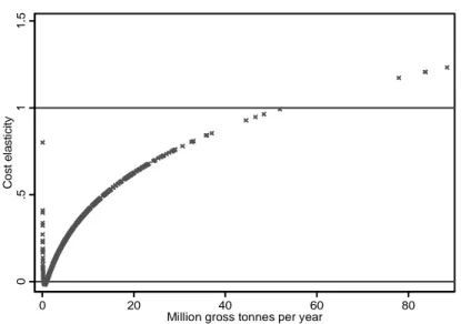
As we have a polynomial for output in terms of total gross tonnes, the elasticity varies with the level of output. Evaluating the cost function at lnTGT and lnTGT2 using expression (9) for each track section and taking the mean gives an elasticity of 0.267; a fraction higher than what has been found in Johansson and Nilsson (2004) and Andersson (2006).

M it it it M it _TGT _TGT TGT C _β _β _β _γ ˆ ) (ln ˆ 3 ln ˆ 2 ˆ ln ln ₂ 3 2 1+ ⋅ ⋅ + ⋅ ⋅ = = ∂ ∂ (9)

A one percent increase in total gross tonnes will increase maintenance costs by 0.267 percent. Caves et al. (1985) defines returns to density (RTD) as the proportional relationship between inputs and outputs with the rail network and prices held constant, which is equivalent to the inverse of the cost elasticity with respect to output (1/ ). RTD are increasing,

constant or decreasing when the elasticity is below, equal or above unity, respectively. A scatter plot of observation specific elasticity estimates is given in figure 2. We can see that we have increasing RTD for most traffic volumes observed. Only track sections with more than 50 million gross tonnes have decreasing RTD.

M it

(20)

Figure 2: Infrastructure maintenance cost elasticities 0 .5 1 1. 5 C o st e la s ti cit y 0 20 40 60 80

Million gross tonnes per year

We also have a positive age effect, but only significant at the 10% level; a percentage increase in rail age increases costs by 0.11 percent.

The F-test supports the model specification at the 5% level and the Breusch-Pagan LM test rejects the hypothesis of zero correlation in the group specific error terms, hence a RE specification is favoured to a POLS. The unobserved effect though is almost as strong for maintenance costs (ρ = 0.87) as for infrastructure operation costs. The Hausman test rejects the assumption of orthogonality between the regressor and the random effect (11.44; prob. value 0.02), hence the FE model is preferred.

4.3 A fixed effects specification for infrastructure maintenance and renewal costs

Finally, we model the aggregate costs of infrastructure maintenance and renewal using the same specification as for maintenance costs only (10) and the results are given in table 7.

it it it it it i MR it TGT TGT TGT RLAGE C =α +β ⋅ln +β ⋅(ln ) +β ⋅(ln ) +β ⋅ln +ε ln ₁ ₂ 2 ₃ 3 ₄ (10)

(21)

The F test signals that this model can be questioned (prob. value 0.22). We have tried

different specifications for the aggregate of maintenance and renewals without improving the model. The cost elasticity of output drops (0.13 at the mean) compared to maintenance only and is no longer significantly positive; a result that is opposite to our expectations and we find difficult to justify. We therefore abstain from commenting this model further.

Table 7. Results from a FE model for infrastructure maintenance and renewal costs

ln TGT 7.018591* (3.974217)

(ln TGT)2 -0.526902* (0.312926)

(ln TGT)3 0.013076 (0.008092)

ln Rail age 0.136496 (0.128273)

F(4, 555) = 1.44 Prob > F = 0.2196

Breusch-Pagan LM Test for Random Effects: χ2 (1) = 536.37 Hausman’s Test for Fixed or Random Effects: χ2

(4) = 15.27 Correlation between unobserved

effect and included covariates = 0.18

σα = 1.095 σε = 0.505 ρ = 0.82

5. Marginal costs and total cost recovery

Swedish and European railway legislation states that prices of infrastructure wear and tear shall be based on direct costs related to utilisation (European Parliament, 2001). The elasticities derived in section 5 can be used to calculate marginal costs. The cost elasticities of output are expressed per train (qt) or gross tonne (qgt), but from a pricing perspective, we prefer the marginal cost to be distance related and expressed in terms of train kilometres (qtkm) or gross tonne kilometres (qgtkm). Following Johansson and Nilsson (2004), we then express the marginal cost for infrastructure operation as (11).

tkm O O it tkm O t O tkm O tkm O tkm O O it q C q C q C q C q C q C MC ⋅ = ⋅ ∂ ∂ = ⋅ ∂ ∂ = ∂ ∂ = ε ln ln ln ln (11)

(22)

The other two cost categories follow in the same fashion. By this, we assume that the cost, at the margin, is unaffected by line length. Estimates of track section marginal costs can be derived by using the elasticity estimates and predicted costs as in (12)

, ˆ ˆ it j it j it j it q C MC =γ ⋅ (12)

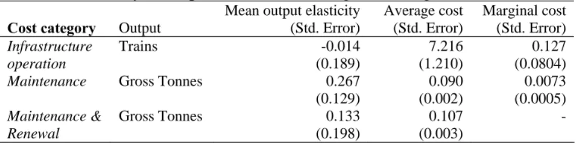
where j indicates the different cost categories and q represents the appropriate output for each model. In order to adjust for the variation of marginal costs over track sections, we calculate a weighted average marginal cost where each track section’s share of total output is used as a weight. This allows the infrastructure manager to use a unit rate for wear-and-tear over the network, and still be revenue neutral to using track section specific marginal costs. Table 8 summarises the main results from our model estimates including calculated weighted average marginal costs.

Table 8. Summary of output elasticities, average and marginal costs Cost category Output

Mean output elasticity (Std. Error) Average cost (Std. Error) Marginal cost (Std. Error) Infrastructure operation Trains -0.014 (0.189) 7.216 (1.210) 0.127 (0.0804)

Maintenance Gross Tonnes 0.267 (0.129) 0.090 (0.002) 0.0073 (0.0005) Maintenance & Renewal Gross Tonnes 0.133 (0.198) 0.107 (0.003) -

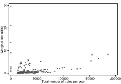
Scatter plots of the predicted marginal costs for infrastructure operation and maintenance are given in figures 3 and 4.

(23)

Figure 3: Marginal infrastructure operation costs 0 10 20 30 M a rg in a l co st (S E K ) 0 50000 100000 150000 200000 Total number of trains per year

Figure 4: Marginal infrastructure maintenance costs

0 .1 .2 .3 .4 M a rg in a l co st ( S E K ) 0 20 40 60 80

Million gross tonnes per year

We can conclude that the mean output elasticities differ substantially between the three cost categories modelled and hence the predicted marginal costs. The marginal cost for infrastructure operation is estimated to SEK 0.13 per train kilometre2. The equivalence for maintenance costs is SEK 0.0073 per gross tonne kilometre. We have not calculated marginal costs for the aggregate of maintenance and renewal model due its poor fit.

2

This estimate includes both positive and negative marginal costs as the marginal cost is a product of elasticities and average costs. In principal this opens up for subsidising low volume tracks and pricing high volume tracks, but such a recommendation is beyond the scope of this paper.

(24)

Cost recovery has been an issue in the rail industry for a long time (Button, 2005) and potential cost recovery is of interest as public infrastructure finances are often constrained. With large fixed costs in the railway industry, pricing at marginal cost will most likely not provide sufficient funds for total cost recovery (Nash, 2003). Cost recovery can be defined as the ratio between marginal and average costs. However, this calculation has to be done at the track section level rather than comparing the two mean estimates in table 8 due to the non-linear relationship between output and cost. Doing this, we estimate the cost recovery from marginal cost pricing of infrastructure operation to approximately 8 percent, while it is around 33 percent for maintenance3. If full cost recovery is aimed at, the gap is large. The current solution is that tax payers cover the gap, but if the gap is to be handled within the rail sector, it requires some innovative financing schemes or maybe an introduction of a fee for scarce capacity where relevant (Nash et al., 2004).

6. Conclusions and discussion

In this paper we have estimated unobserved effects models for railway infrastructure costs in Sweden using a panel of observations over four years. Under the assumption of unobserved infrastructure, managerial and climate effects, we test for a random or fixed effects specification and conclude that the latter is preferable.

Using infrastructure operation costs as dependent variable, we estimate the weighted marginal cost per train kilometre to SEK 0.13. Using infrastructure maintenance costs as dependent variable, we estimate the weighted marginal cost per gross tonne kilometre to SEK 0.0073. These estimates differ from what has previously been estimated by Andersson (2006) using pooled ordinary least squares (POLS). Our model specification tests also reject the POLS in favour of panel data estimators. Adding renewal costs to the dependent variable

3

(25)

leads to insignificant model estimates and we therefore conclude that renewals have to be analysed with a different approach. Even without the inclusion of renewal costs, the marginal cost for maintenance is well above the fee currently in use and an adjustment upwards is justified.

Estimated marginal costs for the different cost categories are generally low compared to average costs, giving rise to a low cost recovery rate. We expect that these low marginal costs arise from existing rules and regulations having a weak relationship with traffic. There are probably large fixed costs for the network manager Banverket before the first train can be dispatched, and a minimum of variable costs for succeeding trains.

In forthcoming research, we will develop the models in this paper further by including dynamic aspects of the planning process as well. Furthermore, we will also look at survival models for rail deterioration in order to explicitly estimate the marginal cost for rail renewal.

It is tough to call for a review of the maintenance strategy at Banverket to place a larger weight on traffic in maintenance decisions, based on this evidence, but asking for a solid data collection strategy is not asking for too much. Rail cost analysis is often hampered by lack of data and deregulation of the railway industry has in fact made the situation even worse (Oum and Waters, 1996). Consistently collecting data over time will give both the research

community and the infrastructure manager a possibility to provide better analyses. Once data is collected in right format, the possibilities open for analyses that can help railway

organisations to fine tune existing infrastructure management and pricing policies.

Acknowledgements

Data provided by Banverket and various train operators in Sweden as well as financial support from Banverket is gratefully acknowledged. This paper has benefited from

(26)

Lars-Göran Mattsson, Gunnar Isacsson and Jan-Eric Nilsson. An earlier version was presented at the Third Conference on Railroad Industry Structure, Competition and Investment, Stockholm School of Economics, 20-22 October, 2005. The author takes sole responsibility for opinions and any remaining errors.

(27)

References

Andersson, M. (2006) Marginal Cost Pricing of Railway Infrastructure Operation, Maintenance and Renewal in Sweden: From Policy to Practice Through Existing Data. Transportation Research Record: Journal of the Transportation Research Board, No. 1943, Transportation Research Board of the National Academies, Washington, D.C., 1-11.

Baltagi, B.H. (2005) Econometric Analysis of Panel Data. 3rd ed., John Wiley & Sons, Chichester, UK.

Banverket (2006) Network Statement. 2006-12-10--2007-12-08(T07), Banverket, Market Division, Borlänge, Sweden.

Banverket (2007) Annual Report 2006. Banverket, Financial Division, Borlänge, Sweden. Bereskin, C.G. (2000) Estimating Maintenance-of-Way Costs for U.S. Railroads After Deregulation. In Transportation Research Record 1707, TRB, National Research Council, Washington, D.C., 13-21.

Berndt, E. and Christensen, L. (1973) The Translog Function and the Substitution of Equipment, Structures and Labor in the US Manufacturing. Journal of Econometrics, 1(1), 81-113.

Bitzan, J.D. (2003) Costs and Competition: The Implications of Introducing Competition to Railroad Networks. Journal of Transport Economics and Policy, 37(2), 201-225.

Breusch, T.S. and Pagan, A.R. (1980) The LM Test and Its Applications to Model Specification in Econometrics. Review of Economic Studies, 47(1), 239-253.

Brown, R.S., Caves, D.W. and Christensen, L.R. (1979) Modelling the Structure of Cost and Production for Multiproduct Firms. Southern Economic Journal, 46(July), 256-273.

Button, K. (2005) The Economics of Cost Recovery. Journal of Transport Economics and Policy, 39(3), 241-257.

Caves, D.W., Christensen, L.R. and Swanson, J.A. (1980) Productivity in U.S. Railroads, 1951-1974. Bell Journal of Economics, 11(1), 168-181.

Caves, D.W., Christensen, L.R., Tretheway, M.W. and Windle, R.J. (1985) Network Effects and the Measurement of Returns to Scale and Density for U.S. Railroads. Chapter 4 in A.F. Daughety (ed.) Analytical Studies in Transport Economics. Cambridge University Press, Cambridge, UK, 97-120.

European Parliament (2001) Directive 2001/14/EC of the European Parliament and of the Council of 26 February 2001 on the Allocation of Railway Infrastructure Capacity and the Levying of Charges for Use of Railway Infrastructure and Safety Certification. Official Journal of the European Communities L 075, March 15, 29-46.

(28)

Griliches, Z. (1972) Cost Allocation in Railroad Regulation. Bell Journal of Economics and Management Science, 3(1), 26-41.

Gujarati, D.N. (1995) Basic Econometrics. 3rd ed., McGraw-Hill, Singapore.

Hausman, J.A. (1978) Specification Tests in Econometrics. Econometrica, 46(6), 1251-1271. Johansson, P. and Nilsson, J.-E. (2004) An Economic Analysis of Track Maintenance Costs. Transport Policy, 11(3), 277-286.

Keeler, T. (1974) Railroad Costs, Returns to Scale, and Excess Capacity. Review of Economics and Statistics, 56(2), 201-208.

Kennedy, J. and Smith, A.S.J. (2004) Assessing the Efficient Cost of Sustaining Britain’s Rail Network: Perspectives Based on Zonal Comparisons. Journal of Transport Economics and Policy, 38(2), 157-190.

Link, H. and Nilsson, J.-E. (2005) Infrastructure. Chapter 3 in Measuring the Marginal Social Cost of Transport, Research in Transportation Economics Vol. 14 (eds. C. Nash and B. Matthews), 49-83.

Nash, C. (2003) Marginal Cost and Other Pricing Principles for User Charging in Transport: A Comment. Transport Policy, 10(4), 345-348.

Nash, C. (2005) Rail Infrastructure Charges in Europe. Journal of Transport Economics and Policy, 39(3), 259-278.

Nash, C., Coulthard, S. and Matthews, B. (2004) Rail Track Charges in Great Britain - The Issue of Charging for Capacity. Transport Policy, 11(4), 315-327.

Oum, T.H. and Waters, W.G. II (1996) A Survey of Recent Developments in Transportation Cost Function Research. Logistics and Transportation Review, 32(4), 423-463.

Regeringen (2006) Moderna transporter. Regeringens Proposition 2005/06:160, Stockholm, Sweden.

Riksdagen (2004) Järnvägslag (2004:519). Stockholm, Sweden.

StataCorp. (2005) Stata Statistical Software: Release 9. College Station, Tx.

Wooldridge, J.M. (2002) Econometric Analysis of Cross Section and Panel Data. MIT Press, Cambridge, Mass.