http://www.diva-portal.org
This is the published version of a paper published in Finite elements in analysis and design
(Print).
Citation for the original published paper (version of record):
Burman, E., Hansbo, P., Larson, M G. (2018)
A simple approach for finite element simulation of reinforced plates
Finite elements in analysis and design (Print), 142: 51-60
https://doi.org/10.1016/j.finel.2018.01.001
Access to the published version may require subscription.
N.B. When citing this work, cite the original published paper.
Open Access
Permanent link to this version:
Finite Elements in Analysis and Design 142 (2018) 51–60
Contents lists available atScienceDirect
Finite Elements in Analysis and Design
journal homepage:w w w . e l s e v i e r . c o m / l o c a t e / f i n e lA simple approach for finite element simulation of reinforced plates
Erik Burman
a, Peter Hansbo
b,*, Mats G. Larson
caDepartment of Mathematics, University College London, London, UK–WC1E 6BT, United Kingdom bDepartment of Mechanical Engineering, Jönköping University, S-551 11, Jönköping, Sweden cDepartment of Mathematics and Mathematical Statistics, Umeå University, SE–901 87, Umeå, Sweden
A R T I C L E I N F O Keywords:
Cut finite element method Discontinuous Galerkin Kirchhoff–Love plate Euler–Bernoulli beam Reinforced plate
A B S T R A C T
We present a new approach for adding Bernoulli beam reinforcements to Kirchhoff plates. The plate is discretised using a continuous/discontinuous finite element method based on standard continuous piecewise polynomial finite element spaces. The beams are discretised by the CutFEM technique of letting the basis functions of the plate represent also the beams which are allowed to pass through the plate elements. This allows for a fast and easy way of assessing where the plate should be supported, for instance, in an optimization loop.
1. Introduction
Reinforcements of plates using lower–dimensional structures such as beams are often employed for the purpose of increasing buckling loads and avoiding eigenfrequencies in vibration problems. The effect of stiffeners can be simulated in a finite element context in a variety of ways. The important issue is how to couple the variables of the beam to the variables of the plate. Different approaches have been suggested: • Point (nodal) constraints matching beam and plate displacements
[20].
• Lagrange multipliers to tie the beam and plate [17].
• Using the plate basis functions also for the beam, along edges or aligned with the elements [5], or obliquely [13,16,19].
The last approach has only been used in the context of Timoshenko beams coupled to Mindlin–Reissner plates, where simple C0 approx-imations can be used; a similar approach was recently suggested for modeling embedded trusses by Lé, Legrain, and Moës [15]. In this paper we present a method for the coupling of Kirchhoff plates and Euler–Bernoulli beams based on this concept, together with a tangential differential approach which simplifies the implementation for arbitrar-ily oriented beams. This is possible thanks to the development of contin-uous/discontinuous Galerkin (c/dG) methods for higher order problems [6,7,9,10], avoiding the use of C1–continuity.
The fact that we do not have to employ higher continuity allows for coupling in other contexts as well. In Ref. [12] we proposed to use the same finite element space for the beam as for the higher dimensional
* Corresponding author.
E-mail address:peter.hansbo@ju.se(P. Hansbo).
structure modeled by linear elasticity, using second order polynomials for elasticity and taking the restriction, or trace, of these polynomials to model the beam using c/dG.
2. Modeling of reinforced plates 2.1. The basic approach
In this Section we develop a simple model of a set of beam elements in a plate. The main approach is as follows:
• Given a continuous finite element space, based on at least second order polynomials for the plate, we define the finite element space for the one–dimensional structure as the restriction of the plate finite element space to the structure which is geometrically modeled by an embedded curve or line.
• To formulate a finite element method on the restricted or trace finite element space we employ continuous/discontinuous Galerkin approximations of the Euler–Bernoulli beam model. The beams are then modeled using the CutFEM paradigm and the stiffness of the embedded beams is in the most basic version, which we consider here, simply added to the plate stiffness.
To ensure coercivity of the cut beam model we in general need to add a certain stabilization term which provides control of the discrete functions variation in the vicinity of the beam. However, for beams embedded in a plate, the plate stabilizes the beam discretizations, and
https://doi.org/10.1016/j.finel.2018.01.001
Received 5 June 2017; Received in revised form 16 November 2017; Accepted 2 January 2018 Available online XXX
we shall show that if the plate is stiff enough compared to the beam the usual additional stabilization [1] is superfluous. The plate problem may also be viewed as an interface problem in order to more accu-rately approximate the plate in the vicinity of the beam structure; this approach is however significantly more demanding from an implemen-tation point of view and we leave it for future work.
The work presented here is an extension of earlier work [4] where membrane structures were considered, in which case a linear approxi-mation in the bulk suffices.
2.2. The Kirchhoff–Love plate model
In the Kirchhoff–Love plate model, posed on a polygonal domain Ω⊂ ℝ2 with boundary𝜕Ω and exterior unit normal n𝜕𝛺, we seek an out–of–plane (scalar) displacement u to which we associate the strain (curvature) tensor
𝜺(∇u) ≔1
2(∇⊗ (∇u) + (∇u) ⊗ ∇) = ∇ ⊗ ∇u = ∇
2u (1)
and the plate stress (moment) tensor
𝝈P(∇u)≔ P (
𝜺(∇u) + 𝜈𝛺(1 −𝜈𝛺)−1div ∇u I) (2)
=P(∇2u +𝜈𝛺(1 −𝜈𝛺)−1ΔuI) (3)
where P=
E𝛺t𝛺3
12(1 +𝜈𝛺) (4)
with E𝛺 the Young’s modulus,𝜈𝛺the Poisson’s ratio, and t𝛺denotes the plate thickness. Since 0≤ 𝜈𝛺≤ 0.5 the constants are uniformly bounded.
The Kirchhoff–Love problem then takes the form: given the out–of–plane load (per unit area) f , find the displacement u such that
div𝐝𝐢𝐯𝝈P(∇u) = f in Ω (5)
u = 0 on𝜕Ω (6)
n𝜕𝛺· ∇u = 0 on𝜕Ω (7)
where𝐝𝐢𝐯 and div denote the divergence of a tensor and a vector field, respectively.
Weak Form. The variational problem takes the form: Find the dis-placement u ∈ VΩ=H02(Ω)such that
aΩ(u, v) = lΩ(v) ∀v ∈ VΩ (8)
where the forms are defined by
aΩ(v, w) = (𝝈P(∇v), 𝜺(∇w))Ω (9)
lΩ(v) = (f, v)Ω (10)
We employ the following notation: L2(𝜔) is the Lebesgue space of square integrable functions on 𝜔 with scalar product (·, ·)L2(𝜔)=
(·, ·)𝜔 and (·, ·)L2(Ω)= (·, ·), and norm ‖·‖L2(𝜔)=‖·‖𝜔 and‖·‖L2(Ω)=‖·‖,
Hs(𝜔) is the Sobolev space of order s on 𝜔 with norm ‖·‖Hs(𝜔),
and H1
0(Ω) = {v ∈ H1(Ω) ∶ v = 0 on𝜕Ω}, and H02(Ω) = {v ∈ H2(Ω) ∶
v = n𝜕𝛺· ∇v = 0 on𝜕Ω}.
2.3. The Euler–Bernoulli beam model
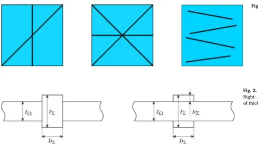
Consider a straight thin beam with centerline Σ⊂ Ω and a rectangu-lar cross-section with width bΣand thickness tΣ, seeFig. 2. The mod-eling of the beam is performed using tangential differential calculus and we follow the exposition in Refs. [11,12], which also covers curved beams. Using this approach the beam equation is expressed in the same coordinate system as the plate, which is convenient in the construction of the cut finite element method for reinforced plates, seeFig. 1for examples.
Let t be the tangent vector to the line Σ and PΣ=t⊗ t the projection onto the one dimensional tangent space of Σ and define the tangential derivatives
∇Σv = PΣ∇v, 𝜕tv = t · ∇v (11)
Then we have the identity
∇Σv = (𝜕tv)t (12)
Based on the assumption that planar cross sections orthogonal to the midline remain plane after deformation we assume that the dis-placement takes the form
u = un +𝜃𝜁t (13)
where𝜁 is the signed orthogonal distance to Ω, positive on one side of Ω and negative on the other side, and𝜃 ∶ Σ → ℝ is an angle representing an infinitesimal rotation, assumed constant in the normal plane.
In Euler–Bernoulli beam theory the beam cross-section is assumed plane and orthogonal to the beam midline after deformation and no shear deformations occur, which means that we have
𝜃 = t · ∇u ≔ 𝜕tu (14)
Fig. 1. Examples of plates reinforced by beams.
Fig. 2. Left: The reinforced plate geometry parameters, tΩ, tΣ, and bΣ.
Right: Alternative design of reinforcement with two separate beams of thickness sΣ= (tΣ−tΩ)∕2 above and below the plate.
E. Burman et al. Finite Elements in Analysis and Design 142 (2018) 51–60
Fig. 3. The meshhwith one beam, the active meshh(Σ)for
the beam in purple, and the set of intersection pointsh(Σ). (For
interpretation of the references to colour in this figure legend, the reader is referred to the Web version of this article.)
This definition for 𝜃 in combination with (13) constitutes the Euler–Bernoulli kinematic assumption
u = un +𝜁(𝜕tu)t = un +𝜁∇Σu
We assume the usual Hooke’s law for one dimensional structural members
𝝈Σ(u) = EΣ𝜺Σ(u) (15) where EΣis the Young modulus and the tangential strain tensor is given by
𝜺Σ(u) = PΣ𝜺(u)PΣ=𝜁𝜺Σ(∇Σu) (16) where in the last equality we used the identity
u⊗ ∇ = (un + 𝜁∇Σu)⊗ ∇ = n ⊗ (∇u) + 𝜁(∇Σu)⊗ ∇ (17) to conclude that
𝜺Σ(u) =𝜁𝜺Σ(∇Σu) (18) Next note that the strain energy density can be written
𝝈Σ(u) ∶𝜺Σ(u) =𝜁2𝝈Σ(∇Σu) ∶𝜺(∇Σu) (19) and the total energy of the beam structure is obtained by integrating over the beam volume
Σ= 1 2∫Σ IΣ𝝈Σ(∇Σu) ∶𝜺(∇Σu) dΣ − ∫ Σ aΣfΣu dΣ (20)
where the integral over the cross section is accounted for by the cross-section area and its second moment
aΣ=bΣtΣ, IΣ=bΣt3Σ∕12 (21)
We are thus led to introducing the beam stress tensor
𝝈B,Σ(∇Σv) = IΣ𝝈Σ(∇Σv) = IΣEΣ𝜺Σ(∇Σv) (22) and thus we have the beam Hooke law
𝝈B,Σ(∇Σv) =B𝜺Σ(∇Σv) (23) where
B=EΣIΣ=
EΣbΣt3Σ
12 (24)
Taking variations we obtain the weak statement, assuming zero displacements and rotations at the end points of Σ, we thus seek u ∈ VΣ=H02(Σ), such that
aΣ(u, v) = lΣ(v) ∀v ∈ VΣ (25)
where the forms are defined by aΣ(v, w) = ∫
Σ𝝈B,Σ
(∇Σv) ∶𝜺Σ(∇Σw) dΣ, lΣ(v) = ∫ Σ
aΣfΣv dΣ (26)
Remark 1. We have the identity
𝜺Σ(∇Σv) = (𝜕2tv)t⊗ t (27)
since (∇Σv)⊗ ∇Σ= ((𝜕tv)t)⊗ ∇Σ= (𝜕t(𝜕tv)t)⊗ t = (𝜕t2v)t⊗ t, where
𝜕t(𝜕tv) =𝜕2tv since t is constant, which leads to
𝝈B,Σ(∇Σv) ∶𝜺(∇Σw) = EΣIΣ𝜕2tv𝜕t2w (28) which leads to aΣ(v, w) = ∫ Σ 𝝈B,Σ(∇Σv) ∶𝜺(∇Σw) dΣ = ∫ Σ EΣIΣ𝜕t2v𝜕2tw dΣ (29) Here we recognize the right hand side as the traditional bilinear form associated with the Euler-Bernoulli beam.
Remark 2. We note that in the alternative reinforcement geometry, right inFig. 2, we have
aΣ=bΣ(tΣ−tΩ), IΣ=
EΣbΣ(t3Σ−t3Ω)
12 (30)
We may also consider more complicated cross sections and compute the proper parameters.
Remark 3. We assume that the beam centerline is located in the sym-metry plane of the plate, seeFig. 2, which simplifies the modeling of a reinforced plate since it will be subject to pure bending. If the beams are located on one side of the plate the main approach is the same but we must include models for the membrane deformation of the plate and beams.
2.4. The reinforced plate model
Let = {S} be a set of beams arbitrarily oriented in Ω. Using super-position we obtain the problem: find u ∈ V such that
a(u, v) = l(v) ∀v ∈ V (31) where V = VΩ ⋂ Σ∈ VΣ (32)
and the forms are defined by a(v, w) = aΩ(v, w) + ∑ Σ∈ aΣ(v, w) (33) l(v) = lΩ(v) + ∑ Σ∈ lΣ(v) (34)
Remark 4. Note that for the alternative plate reinforcement geometry, right inFig. 2, there is no geometric error in our method if we use the parameters(30). In the standard reinforcement geometry, left inFig. 2, there is a however a geometric error proportional to bΣ in the plate bilinear form, which arises in the superposition since the intersection between the beam and the plate is nonempty. We will later see that bΣ typically is smaller (in practice significantly smaller) than the mesh size since we are using thin beam and plate theory, see(35), and thus the geometric error is small.
3. Finite element discretization 3.1. The mesh and finite element spaces
• We consider a subdivisionh= {T} of Ω into a geometrically con-forming finite element mesh, with mesh parameter h ∈ (0, h0]. We assume that the elements are shape regular, i.e., the quotient of the diameter of the smallest circumscribed sphere and the largest inscribed sphere is uniformly bounded. We denote by hT the diam-eter of element T and by h = maxT∈hhT the global mesh size parameter.
• Since we are using thin plate and beam theory we assume that there is a constant Cmeshsuch that
Cmeshmax(tΩ, tΣ, bΣ)≤ h (35)
• We shall use continuous, piecewise polynomial approximations, for both the membrane and plate problem. Let
VΩ,h,k= {v ∈ C0(Ω) ∶ v∣T∈k(T) ∀T ∈ } (36) wherek(T) is the space of polynomials of degree less or equal to k defined on T. For simplicity, we write VΩ,h=VΩ,h,k.
• To define our method we introduce the set of faces (edges) F in the mesh,h= {F}, and we splithinto two disjoint subsets
h=h,I∪h,B (37)
whereh,Iis the set of faces in the interior of Ω andh,Bis the set of faces on the boundary.
• Further, with each face F we associate a fixed unit normal nFsuch that for faces on the boundary nFis the exterior unit normal. We denote the jump of a function v at a face F by [v] = v+−v− for
F ∈h,Iand [v] = v+for F ∈
h,B, and the average⟨v⟩ = (v++v−)∕2 for F ∈h,Iand⟨v⟩ = v+for F ∈h,B, where v±=lim𝜖↓0v(x ∓𝜖 nF) with x ∈ F.
• Given a line segment Σ in Ω that represents a beam we let h(Σ) = {T ∈h∶T ∩ Σ≠ ∅}
and we leth(Σ)be the set of all interior faces inh(Σ).
• The intersection points between Σ and element faces in h(Σ) is denoted
h(Σ) = {x ∶ x = F ∩ Σ, F ∈ h(Σ)} (38)
and we assume that this is a discrete set of points (thus excluding the case where any F ∈hcoincides with a part of Σ), seeFig. 3for illustration.
Remark 5. The assumption(35)is natural since we use models for thin structures as our basis for the finite element discretization. In particular, in(71)we use the estimate bΣ≤ Ch which means that the mesh size can not become very small in comparison to the beam width. If that would happen the modeling of the beam as a form based on the beam centerline would not be reasonable and a more detailed model should be used as the basis for finite element modeling.
3.2. The c/dG method for the plate
We approximate the solution to the plate problem using the continu-ous/discontinuous Galerkin (c/dG) method: Find uh∈VΩ,h, with k≥ 2, such that
aΩ,h(uh, v) = lΩ(v) ∀v ∈ VΩ,h (39) The bilinear form aΩ,h(·, ·) is defined by
Fig. 4. Beam reinforced plate.
Fig. 5. Computational mesh.
aΩ,h(v, w) = ∑ T∈h (𝝈P(∇v), 𝜺(∇w))T − ∑ F∈h,I∪h,B (⟨nF·𝝈P(∇v)⟩, [∇w])F − ∑ F∈h,I∪h,B ([∇v], ⟨nF·𝝈P(∇w)⟩)F + ∑ F∈h,I∪h,B 𝛽𝛺h−1F ([∇v], [∇w])F (40) Here𝛽𝛺is a positive parameter of the form
𝛽𝛺=𝛽Ω,0P=𝛽Ω,0
E𝛺t3 𝛺
12(1 +𝜈𝛺) (41)
where𝛽Ω,0is a constant depending on the polynomial order k, see Ref. [10] for details, and hFis defined on each face F by
hF= (
|T+| + |T−|)
∕(2|F|) for F = 𝜕T+∩𝜕T− (42)
with|T| the area of T and |F| the length of F.
Remark 6. The idea of using continuous/discontinuous approxima-tions was first proposed by Engel et al. [6] and later analysed for Kirchhoff–Love and Mindlin–Reissner plates in Refs. [7,9,10], cf. also Wells and Dung [21].
E. Burman et al. Finite Elements in Analysis and Design 142 (2018) 51–60
Fig. 6. Beam/mesh intersection at the center.
Remark 7. Other boundary conditions for plates, for instance simply supported and free, can easily be included in the c/dG finite element method, see Ref. [8] for details.
Remark 8. For v ∈ VΩ,hwe have [∇v] = [nF· ∇v]nFsince v is continu-ous across a face and v = 0 on𝜕Ω. Therefore
(⟨nF·𝝈(∇v)⟩, [∇w])F= (⟨nF·𝝈(∇v) · nF⟩, [nF· ∇w])F (43) for all v, w ∈ VΩ,h, and we note that (nF·𝝈(∇u) · nF)|F is the bending moment at the edge F.
3.3. The cut c/dG method for a beam
We propose the following cut c/dG method. Find uh∈VΣ,h= VΩ,h|h(Σ)such that
AΣ,h(uh, v) = lΣ(v) ∀v ∈ VΣ,h (44) where the forms are defined by
AΣ,h(v, w) = aΣ,h(v, w) + sΣ,h(v, w) (45) aΣ,h(v, w) = ∑ T∈h(Σ) (𝝈B,Σ(∇Σv), 𝜺(∇Σw))Σ∩T − ∑ x∈h(Σ) (⟨t · 𝝈B,Σ(∇Σv)⟩, [∇Σw])x − ∑ x∈h(Σ) ([∇Σv], ⟨t · 𝝈B,Σ(∇Σw)⟩)x + ∑ x∈h(Σ) 𝛽Σh−1([∇Σv], [∇Σw])x (46) sΣ,h(v, w) = ∑ F∈h,I(Σ) k ∑ j=0 2 ∑ i=0 h2j‖[𝜕j nF𝜕 i tv]‖2F + ∑ T∈h,I(Σ) 2 ∑ i=0 𝛾Σ,2h(𝜕nΣ𝜕 i tv, 𝜕nΣ𝜕 i tw)T (47)
Here we used the notation (v, w)x=v(x)w(x), the penalty parameter takes the form
𝛽Σ=𝛽Σ,0B=𝛽Σ,0EΣIΣ (48)
with𝛽Σ,0a parameter that only depends on the polynomial order, and
sΣ,his a stabilization form with positive parameters
𝛾Σ,i=𝛾Σ,i,0B=𝛾Σ,i,0EΣIΣ, i = 1, 2 (49) The form sΣ,his added to ensure coercivity and stability of the stiffness matrix, cf. [1], in the case when the beam is not embedded in a plate
or if the plate is very weak. For completeness we provide an analysis of this case, which also motivates the form of the stabilization form, in Appendix Abelow.
Remark 9. Using the identities
∇Σv = (𝜕tv)t, 𝜺Σ(∇Σv) = (𝜕2tv)t⊗ t, 𝝈B,Σ(∇Σv) = EΣIΣ(𝜕t2v)t⊗ t (50) we note that aΣ,hcan alternatively be written in the form
aΣ,h(v, w) = ∑ T∈h(Σ) (EΣIΣ𝜕t2v, 𝜕2tw)Σ∩T − ∑ x∈h(Σ) (⟨EΣIΣ𝜕t2v⟩, [𝜕tw])x − ∑ x∈h(Σ) ([𝜕tv], ⟨EΣIΣ𝜕t2w⟩)x + ∑ x∈h(Σ) 𝛽Σ,0 h (EΣIΣ[𝜕tv], [𝜕tw])x (51) which is the form in Ref. [6].
Remark 10. The terms on the discrete seth(Σ)are associated with the work of the end moments on the end rotation which occur due to the lack of C1(Ω)continuity of the approximation, as in the plate model. SeeRemark 8.
Remark 11. We note that due to the stabilization this method works for a single beam, i.e. without being embedded in a plate. The basic principle is the same as for the trace finite element method proposed in Ref. [18] and the stabilized version proposed in Ref. [2]. When the beam is embedded in a plate, which is the case in this work, the need for the stabilization term is mitigated, and if the plate is sufficiently stiff we may omit the stabilization term, see Section 3.5for further details.
3.4. The c/dG method for the reinforced plate model
Recall that = {Σ} is a set of beams arbitrarily oriented in Ω. Using superposition we obtain the problem: find uh∈VΩ,hsuch that
Ah(uh, v) = l(v) ∀v ∈ VΩ,h (52)
where the forms are defined by Ah(v, w) = aΩ,h(v, w) + ∑ Σ∈ aΣ,h(v, w) (53) l(v) = lΩ(v) + ∑ Σ∈ lΣ(v) (54)
3.5. Coercivity for reinforced plates
In this section we study the coercivity of the c/dG method for the reinforced plate. We shall use the stability provided by the plate to prove stability of the reinforced plate, without the need of the stabi-lizing terms (𝛾Σ,1=𝛾Σ,2=0). This is only possible as long as the mesh size h is larger than or equal to the beam with bΣ. When this condition is not satisfied, stability uniform in h is achieved only when the stabi-lizing terms are included (𝛾Σ,1, 𝛾Σ,2> 0), using similar ideas as in Refs. [2,3].
Coercivity of the Plate. We first recall that the c/dG method for the plate is coercive. Introducing the energy norm
|||v|||2 Ω,h= ∑ T∈h P‖∇2v‖2T+ ∑ F∈h Ph‖⟨∇2v⟩‖2F+ ∑ F∈h Ph−1‖[∇v]‖2F (55) there is a constant mP> 0 such that
mP|||v|||2Ω,h≤ aΩ,h(v, v) ∀v ∈ VΩ,h (56)
for𝛽Ωlarge enough.
Fig. 7. Displacements using simply supported support for the beams, EΣ=100EΩ(left) and EΣ=1000EΩ(right).
Fig. 8. Displacements using fixed support for the beams, EΣ=100EΩ(left) and EΣ=1000EΩ(right).
Coercivity of the Reinforced Plate. Next turning to the reinforced plate we introduce the energy norm associated with the beam
|||v|||2 Σ,h= ∑ T∈h(Σ) B‖𝜕t2v‖2Σ∩T+ ∑ x∈h(Σ) Bh‖⟨𝜕t2v⟩‖2x + ∑ x∈h(Σ) Bh−1‖[𝜕tv]‖2x (57)
Then there is a constant m such that
m(|||v|||2Σ,h+|||v|||2Ω,h)≲ Ah(v, v) ∀v ∈ Vh (58) for𝛽Ωand𝛽Σlarge enough.
Verification of (58), Using the following two inequalities, which we verify below, C1 ( ∑ x∈h(Σ) Bh‖⟨𝜕t2v⟩‖2x ) ≤ ∑ T∈h P‖∇2v‖2T (59)
for some constant C1> 0, and ∑ T∈h(Σ) B‖𝜕t2v‖2Σ∩T+ ∑ x∈h(Σ) Bh−1‖[𝜕tv]‖2x ≤ ∑ T∈h mP 3 P‖∇ 2v‖2 T+aΣ,h(v, v) (60)
for𝛽Σlarge enough, we have
Ah(v, v) = aΩ,h(v, v) + aΣ,h(v, v) (61) ≥ mP|||v|||2Ω,h+aΣ,h(v, v) (62) =mP 3 |||v||| 2 Ω,h+ mP 3 |||v||| 2 Ω,h+ (m P 3 |||v||| 2 Ω,h+aΣ,h(v, v) ) (63) ≥mP 3 |||v||| 2 Ω,h+ C1mP 3 ( ∑ x∈h(Σ) Bh‖⟨𝜕2tv⟩‖2x ) (64) + ⎛ ⎜ ⎜ ⎝ ∑ T∈h(Σ) B‖𝜕2tv‖2∩T+ ∑ x∈h(Σ) Bh−1‖[𝜕tv]‖2x ⎞ ⎟ ⎟ ⎠ ≥ m(|||v|||2 Σ,h+|||v||| 2 Ω,h ) (65) where m = min(mP∕3, C1mP∕3, 1).
Verification of(59). We note that, for a point x ∈ Σ ∩ T, T ∈h, we have the estimates
‖𝜕2
E. Burman et al. Finite Elements in Analysis and Design 142 (2018) 51–60 where used the fact that t is a constant unit vector so that 𝜕2
tv =
t · (∇2v) · t ∈
k−2(T) is a well defined expression on T since v ∈k(T) is a polynomial on T then we used an inverse inequality to pass from the point value to the L2norm on the element T. For instance, in the important case of quadratic elements ∇2v is a constant and for a con-stant function w we have the estimate
‖w‖2
x=w2(x) =|T|−1|T|w2(x) =|T|−1‖w‖2T≲ h−2‖w‖2T (67) since it follows from shape regularity of T and quasiuniformity of the mesh that the element area|T| ∼ h2.
Using(66) we obtain, withh(x) = {T ∈h∶x ∈ T} the set of all elements such that x ∈ T,
∑ x∈h(Σ) Bh‖⟨𝜕t2v⟩‖2x≤ ∑ x∈h(Σ) C2 inv B PhP‖∇ 2v‖2 h(x) (68) ≤ C2 inv B Ph|||v||| 2 Ω,h (69)
and thus we have the estimate 1 C2 inv Ph B ⏟⏞⏞⏟⏞⏞⏟ C1 ( ∑ x∈h(Σ) Bh‖⟨𝜕2tv⟩‖2x ) ≤ |||v|||2 Ω,h (70)
We note, using the definitions(4)and(24)ofPandB, that Ph B = 1 1 +𝜈𝛺 E𝛺t3 Ω EΣt3Σ h bΣ ≥ 1 1 +𝜈𝛺 E𝛺t3 Ω EΣtΣ3 Cmesh (71)
where we used the condition that the beam width is smaller than the mesh size(35)and thus the right hand side is a positive constant inde-pendent of the mesh size and so is C1.
Verification of(60). First we have the equality aΣ,h(v, v) = ∑ T∈h(Σ) B‖𝜕2tv‖2Σ∩T −2 ∑ x∈h(Σ) B(⟨𝜕t2v⟩, [𝜕tv])x ⏟⏞⏞⏞⏞⏞⏞⏞⏞⏞⏞⏞⏞⏞⏞⏞⏟⏞⏞⏞⏞⏞⏞⏞⏞⏞⏞⏞⏞⏞⏞⏞⏟ ★ + ∑ x∈h(Σ) 𝛽Σ,0Bh−1‖[𝜕tv]‖2x (72) To estimate★ we employ the inverse inequality(66)as follows
★ = 2 ∑ x∈h(Σ) B(⟨𝜕t2v⟩, [𝜕tv])x (73) ≤ 2 ∑ x∈h(Σ) BCinvh−1‖∇2v‖h(x)‖[𝜕tv]‖x (74) ≤ ∑ T∈h(Σ) 𝛿BC2invh−1‖∇2v‖2T + ∑ x∈h(Σ) 𝛿−1 Bh−1‖[𝜕tv]‖2x (75)
where we used the inequality ab≤ (𝛿a2+𝛿−1b2)∕2 for𝛿 > 0. We then obtain(60)as follows ∑ T∈h mP 3P‖∇ 2v‖2 T+aΣ,h(v, v) ≥ ∑ T∈h(Σ) B‖𝜕2tv‖2Σ∩T + ∑ T∈h (m P 3P−𝛿BC 2 invh −1) ⏟⏞⏞⏞⏞⏞⏞⏞⏞⏞⏞⏞⏞⏞⏞⏞⏟⏞⏞⏞⏞⏞⏞⏞⏞⏞⏞⏞⏞⏞⏞⏞⏟ ≥0 ‖∇2v‖2 T + ∑ x∈h(Σ) (𝛽Σ,0−𝛿−1) ⏟⏞⏞⏞⏞⏟⏞⏞⏞⏞⏟ ≥1 Bh−1‖[𝜕tv]‖2x (76)
Fig. 9. Beam reinforced plate.
Fig. 10. Computational mesh.
≥ ∑ x∈h(Σ) Bh−1‖[𝜕tv]‖2x+ ∑ x∈h(Σ) Bh−1‖[𝜕tv]‖2x (77)
Here we choose:𝛿 small enough to guarantee that 0≤mP 3 P−𝛿BC 2 invh−1= mP 3 P ( 1 −𝛿 3 mP BC2inv Ph ) =mP 3 P ( 1 −𝛿 3 mP 1 C1 ) (78) where as above, see(71), C1> 0 independent of the mesh parameter h, and𝛽Σsuch that
𝛽Σ− 1
𝛿≥ 1 (79)
4. Numerical examples
In this section, we give some elementary examples of what can be achieved with the presented technique. In all numerical examples we use polynomial order 2, fΣ=0, and
fΩ=8P(3(x2(1 − x)2+y2(1 − y)2) + (1 − 6x(1 − x))(1 − 6y(1 − y))) corresponding to the solution u = x2(1 − x)2y2(1 − y)2 for a clamped plate unsupported by beams.
In order to handle more general boundary conditions we in partic-ular need to be able to impose end displacements on the beam in the
Fig. 11. Deformations when the beams are clamped at x = 1.
Fig. 12. Deformations when all beams are clamped.
case of a free plate (we note that strongly imposed boundary conditions on the plate are also enforced on the beam). Zero displacement of the beam endpoints xEare imposed by adding penalty terms
̃ 𝛽Σ,0
h3 (EΣIΣv, w)xE (80)
to the form aΣ,h(v, w) in(51), where ̃𝛽Σ,0is a penalty parameter. These terms suffice for optimal order convergence (of the beam approxima-tion) in the case of second degree polynomial approximations since the shear forces required for energy consistency are third derivatives of dis-placements, and thus equal zero.
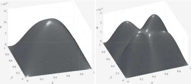
4.1. Simply supported plate using beams with different supports
We consider a simply supported plate on the domain Ω = (0, 1) × (0, 1) with Young’s modulus EΩ=100, Poisson’s ratio𝜈Ω=1∕2, and
Fig. 13. Deformations when all beams are simply supported.
thickness tΩ=0.1. The plate is supported by two beams oriented as inFig. 4, one at x = 0.499 and one at y = 0.499 (to avoid intersection with the mesh lines). The computational mesh is shown inFig. 5and in Fig. 6were show a close-up of the intersection between the beams and the mesh.
For this problem we test two different supports for the beams: sim-ply supported and fixed, and two different stiffnesses for the beams: EΣ=100EΩand EΣ=1000EΩ. The thickness and width of the beam are equal and the same as the thickness of the plate. InFig. 7we show the results using EΣ=100EΩ, with simply supported and fixed supports; in Fig. 8we show the results using EΣ=1000EΩ, with simply supported and fixed supports.
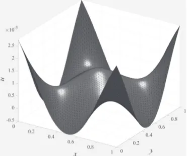
4.2. Plate only supported by beams
Next, we consider a plate with free boundaries, supported only by beams. All data for the plate are the same as in the previous exam-ple. The plate is supported by four beams positioned at 1∕3 and 2∕3 from each boundary as indicated inFig. 9. The beams have the same dimension as previously, with Young’s modulus EΣ=100EΩ. The com-putational mesh is unstructured and shown inFig. 10.
We first consider the case when the beams are clamped at x = 1 and free elsewhere. InFig. 11we see an elevation of the corresponding deformation. Next we consider the case when all beams are clamped, Fig. 12, and simply supported,Fig. 13. Note the slight increase in cen-tral displacement for the latter.
5. Conclusions
We have formulated a continuous/discontinuous Galerkin method for beam reinforced thin plates. The method has the advantage that we can discretize both the beam and plate problem with the same standard finite element spaces of continuous piecewise polynomials defined on triangles (or quadrilaterals).
Acknowledgement
This research was supported in part by the Swedish Foundation for Strategic Research Grant No. AM13-0029, the Swedish Research Council Grant No. 2013-4708, and the Swedish strategic research pro-gramme eSSENCE. The first author was supported in part by EPSRC grant EP/P01576X/1.
E. Burman et al. Finite Elements in Analysis and Design 142 (2018) 51–60 Appendix A. Coercivity for beams which are not embedded in a plate
To prove coercivity of the bilinear form associated with the beam AΣ,h, defined in(45), in the case when the beam is not embedded in a plate we utilize the stabilization term sΣ,h, see(47), which provides the following estimate
∑ T∈h(Σ) 2 ∑ j=0 Bh−1‖𝜕jtv‖2T≤ Cstab (2 ∑ j=0 B‖𝜕2tv‖2Σ+‖v‖ 2 sΣ,h ) (A.1) where‖v‖2
sΣ,h=sΣ,h(v, v). Starting from(72)we use the first inequality in(66)followed by(A.2)to estimate★ as follows
★ = 2 ∑ x∈h(Σ) B(⟨𝜕t2v⟩, [𝜕tv])x (A.2) ≤ 2 ∑ x∈h(Σ) BCinvh−1‖𝜕t2v‖h(x)‖[𝜕tv]‖x (A.3) ≤ ∑ T∈h(Σ) 𝛿BC2invh −1‖𝜕2 tv‖2T+ ∑ x∈h(Σ) 𝛿−1 Bh−1‖[𝜕tv]‖2x (A.4) ≤ 𝛿C2 invCstab ⎛ ⎜ ⎜ ⎝ ∑ T∈h(Σ) B‖𝜕t2v‖2Σ∩T+‖v‖ 2 sΣ,h ⎞ ⎟ ⎟ ⎠ + ∑ x∈h(Σ) 𝛿−1 Bh−1‖[𝜕tv]‖2x (A.5)
Now choosing𝛿 small enough and 𝛽Σ,0large enough we obtain the coercivity estimate ∑ T∈h(Σ) B‖𝜕t2v‖Σ∩2 T+‖v‖2sΣ,h+ ∑ x∈h(Σ) Bh‖⟨𝜕2tv⟩‖2x+ ∑ x∈h(Σ) Bh−1‖[𝜕tv]‖2x≲ AΣ,h(v, v) (A.6)
for all v ∈ VΣ,h. For completeness we include the main steps in the derivation of(A.1). For related results we refer to [3] and [14]. • For an element T with a so called large intersection with Σ, that is|T ∩ Σ| ≳, it holds, for v ∈ k(T),
‖v‖2 T≲ h‖v‖2T∩Σ+h2‖𝜕nΣv‖ 2 F (A.7) Setting v =𝜕i tw, i = 0, 1, 2, we get 2 ∑ i=0 h−1‖𝜕i tw‖2T≲ ‖𝜕 i tw‖2T∩Σ+ 2 ∑ i=0 h‖𝜕nΣ𝜕 i tw‖2T (A.8)
• For two elements T1and T2which share the face F it holds, for all w1∈Pk(T1)and w2∈Pk(T2), ‖w1‖2T1≲ ‖w2‖ 2 T2+ k ∑ j=0 h2j+1‖[𝜕njFw]‖2F (A.9)
see Ref. [12]. Setting w =𝜕i
tv, i = 0, 1, 2, we obtain 2 ∑ i=0 h−1‖𝜕i tv‖2T1≲ 2 ∑ i=0 h−1‖𝜕i tv‖2T2+ k ∑ j=0 2 ∑ i=0 h2j‖[𝜕j nF𝜕 i tv]‖2F (A.10)
• To prove the stability estimate(A.1)we note that it follows from quasi uniformity that for each element T ∈h(Σ)there is a path of elements {Ti}ni=0, with length n uniformly bounded, such that T0=T, Tiand Ti+1share a face, and Tnhas a large intersection with Σ. Using(A.10)to pass between the elements in the path and then finally using(A.8)we obtain(A.1).
References
[1] E. Burman, S. Claus, P. Hansbo, M.G. Larson, A. Massing, CutFEM: discretizing geometry and partial differential equations, Int. J. Numer. Meth. Eng. 104 (7) (2015) 472–501.
[2] E. Burman, P. Hansbo, M.G. Larson, A stabilized cut finite element method for partial differential equations on surfaces: the Laplace-Beltrami operator, Comput. Meth. Appl. Mech. Eng. 285 (2015) 188–207.
[3] E. Burman, P. Hansbo, M.G. Larson, A. Massing, Cut finite element methods for partial differential equations on embedded manifolds of arbitrary codimensions, ArXiv e-prints (Oct. 2016).
[4] M. Cenanovic, P. Hansbo, M.G. Larson, Cut finite element modeling of linear membranes, Comput. Meth. Appl. Mech. Eng. 310 (2016) 98–111.
[5] A. Deb, M. Booton, Finite element models for stiffened plates under transverse loading, Comput. Struct. 28 (3) (1988) 361–372.
[6] G. Engel, K. Garikipati, T.J.R. Hughes, M.G. Larson, L. Mazzei, R.L. Taylor, Continuous/discontinuous finite element approximations of fourth-order elliptic problems in structural and continuum mechanics with applications to thin beams and plates and strain gradient elasticity, Comput. Meth. Appl. Mech. Eng. 191 (34) (2002) 3669–3750.
[7] P. Hansbo, D. Heintz, M.G. Larson, A finite element method with discontinuous rotations for the Mindlin-Reissner plate model, Comput. Meth. Appl. Mech. Eng. 200 (5–8) (2011) 638–648.
[8] P. Hansbo, M.G. Larson, A discontinuous Galerkin method for the plate equation, Calcolo 39 (1) (2002) 41–59.
[9] P. Hansbo, M.G. Larson, A P2-continuous, P1-discontinuous finite element method for the Mindlin-Reissner plate model, in: F. Brezzi, A. Buffa, S. Corsaro, A. Murli (Eds.), Numerical Mathematics and Advanced Applications, Springer Italia, Milan, 2003, pp. 765–774.
[10]P. Hansbo, M.G. Larson, A posteriori error estimates for continuous/discontinuous Galerkin approximations of the Kirchhoff-Love plate, Comput. Meth. Appl. Mech. Eng. 200 (47–48) (2011) 3289–3295.
[11]P. Hansbo, M.G. Larson, K. Larsson, Variational formulation of curved beams in global coordinates, Comput. Mech. 53 (4) (2014) 611–623.
[12]P. Hansbo, M.G. Larson, K. Larsson, Cut finite element methods for linear elasticity problems, ArXiv e-prints (2017) abs/1703.04377.
[13]T. Holopainen, Finite element free vibration analysis of eccentrically stiffened plates, Comput. Struct. 56 (6) (1995) 993–1007.
[14]M.G. Larson, S. Zahedi, Stabilization of higher order cut finite element methods on surfaces, ArXiv e-prints (Oct. 2017).
[15] B. Lé, G. Legrain, N. Moës, Mixed dimensional modeling of reinforced structures, Finite Elem. Anal. Des. 128 (2017) 1–18.
[16] A. Mukherjee, M. Mukhopadhyay, Finite element free vibration of eccentrically stiffened plates, Comput. Struct. 30 (6) (1988) 1303–1317.
[17] J.R. O’Leary, I. Harari, Finite element analysis of stiffened plates, Comput. Struct. 21 (5) (1985) 973–985.
[18] M.A. Olshanskii, A. Reusken, J. Grande, A finite element method for elliptic equations on surfaces, SIAM J. Numer. Anal. 47 (5) (2009) 3339–3358. [19] G. Palani, N.R. Iyer, T. Appa Rao, An efficient finite element model for static and
vibration analysis of plates with arbitrarily located eccentric stiffeners, J. Sound Vib. 166 (3) (1993) 409–427.
[20] M. Rossow, A. Ibrahimkhail, Constraint method analysis of stiffened plates, Comput. Struct. 8 (1) (1978) 51–60.
[21] G.N. Wells, N.T. Dung, A C0discontinuous Galerkin formulation for Kirchhoff plates, Comput. Meth. Appl. Mech. Eng. 196 (35–36) (2007) 3370–3380.