Equation-Based Modeling of FACTS using Modelica

http://www.diva-portal.org

Postprint

This is the accepted version of a paper presented at PowerTech Eindhoven 29 June - 2 July 2015.

Citation for the original published paper:

Adib Murad, A., Gómez, F J., Vanfretti, L. (2015)

Equation-Based Modeling of FACTS using Modelica.

In: IEEE conference proceedings

http://dx.doi.org/10.1109/PTC.2015.7232500

N.B. When citing this work, cite the original published paper.

Permanent link to this version:

Equation-Based Modeling of FACTS using Modelica

KTH, Royal Institute of Technology, Stockholm, Sweden

maamurad@kth.se , fragom@kth.se , luigiv@kth.se

Luigi Vanfretti

KTH Royal Institute of Technology, Stockholm, Sweden Statnett SF, Oslo, Norway

luigi.vanfretti@kth.se, luigi.vanfretti@statnett.no

Abstract— This paper reports results of extending the iTesla

Modelica Power System Library with the implementation of new Modelica models for power electronic-based FACTS (Flexible AC Transmission System) to be used in phasor time-domain simulations. To show the applicability of Modelica for modeling FACTS devices and power system simulation, a software-to-software validation is performed against the Power System Analysis Toolbox (PSAT), which is used as the reference software for validation. A quantitative and qualitative assessment of the validation results between PSAT and Modelica is given.

Index terms – Modelica, PSAT, FACTS Devices, Power System Simulation

I. INTRODUCTION

A. Motivation

Modern electric power systems are one of the most complex networked systems, their role is to ensure continuous supply of electricity. For the planning and operation of this complex networks, modeling and simulation are essential to satisfy operational requirements or planning constraints [1], [2]. Power system models used in time-domain simulations can be categorized into different types: Electro-Magnetic Transient type, Phasor Time Domain type or Quasi Steady State type [3], [4]. The modeling approach may also vary depending on the kind of studies to be performed or the simulation's solver. In the later case, a particular choice of solver may influence the modeling approach, making it difficult to evaluate the quality of the model among different tools that are used for the same kind of studies [1].

Existing simulation tools are exposed to different limitations such as: limited abilities for consistent model exchange [5], availability of simulation features [2], and accessibility to internal component model implementation for modification and/or inefficient handling of new implemented devices. As an example, the discrepancy between two EMT tools (PSCAD and Matlab/Simulink) is presented in [6].

Complex physical phenomena arising in power systems must be analyzed with detailed computer-based simulations [7]. Proprietary or closed-source power system simulation software packages like PSS/E, PSCAD and others, do not allow to change the source code or to modify existing internal

models [8]. To increase the flexibility of power system simulation software’s, the Open Source Software (OSS) development approach is attractive. Some examples of OSS are UWPFLOW [9], PSAT [10], PowerWeb [11], ObjectStab [12]. However, some of these are no longer supported and/or incompatible with the language's compiler [13].

B. The choice of Modelica as a language for power sytem modeling

To overcome the previous limitations, the Modelica language is a promising option. Modelica is an object-oriented, open-source, equation-based modeling language, which has been successfully applied to automotive and aerospace industry [14]. Modelica and related Modelica tools, e.g. OpenModelica, Dymola, SystemModeler, and others; offer attractive features for power system simulation and they allow model information exchange between different simulation tools. This is because a Modelica model is decoupled from any mathematical solver. Taking into account this characteristic, a Modelica model accepts modifications in its equations and its parameters, and provides unambiguous simulation results among different simulations tools [1]. European transmission system security is becoming a challenge due to the growing complexities of the pan-European power network. To overcome these complexities, the FP7 iTesla (Innovative Tools for Electrical System Security within Large Areas) project was initiated to develop a toolbox that will support the operation of the European transmission network [15]. The iTesla project has adopted the Modelica language for modeling of power system dynamic components, and a Modelica library compatible with Modelica tools has been developed. This library includes models with reference Eurostag, PSS/E and PSAT.

C. Contributions of this paper

Modeling of FACTS devices is addressed in this paper. The validation of these models takes as a reference their mathematical model and implementation in PSAT [16]. In addition, the IEEE 9-Bus Test System has been used to test the performance of the FACTS devices implemented in Modelica. A Modelica model of this 9-Bus test system has been implemented and validated against its equivalent PSAT model. A quantitative and qualitative assessment between the simulations results of Modelica and PSAT is given.

This work was supported in part by the EU-funded FP7 iTESLA project and by Statnett SF, the Norwegian Transmission System Operator, under grant agreement n°283012. iTESLA (Innovative Tools for Electrical System Security within Large Areas), online: www.itesla-project.eu

Furthermore, analysis of the use of different solvers available in Modelica tools against the trapezoidal integration method in PSAT is shown to highlight the value of decoupling the mathematical model of the power system from mathematical solvers.

II. DETAILS OF THE FACTS DEVICES

The FACTS devices addressed here are: Static Synchronous Compensator (STATCOM), Thyristor Controlled Series Compensator (TCSC), Static Synchronous Source Series Compensator (SSSC) and Unified Power Flow Controller (UPFC). For the implementation for these models in Modelica, the mathematical description of these models in [16] has been taken as reference. These models are averaged valued models, as in PSAT. This is because in phasor time-domain simulation the aim is to observe the phenomena of power system network with FACTS devices without describing in detail of the underlying switching of the power electronics in these devices.

A. STATCOM (Static Synchronous Compensator)

A STATCOM is a shunt-connected FACTS device used to regulate the voltage of the bus that it is connected to, therefore only reactive power is exchanged between the AC system and the device. The reference model is a controlled current injector as depicted in Fig.1.

1 r r K T s max i min i v ref v POD s v SH i SH i

Figure 1: Control Block diagram of STATCOM [16].

The differential equation that describes the behavior of the STATCOM is given by:

𝑑(𝑖𝑆𝐻)

𝑑𝑡 = (𝐾𝑟(𝑣𝑟𝑒𝑓+ 𝑣𝑠

𝑃𝑂𝐷_{− 𝑣) − 𝑖}

𝑆𝐻)/𝑇𝑟 (1)

which influences the reactive power injection, given by 𝑞 = 𝑖𝑆𝐻∗ 𝑣 (2)

here, 𝑖_𝑆𝐻 is the injected current, 𝑣 is bus voltage, 𝐾_𝑟 is regulator gain, 𝑇𝑟 is regulator time constant, 𝑣𝑟𝑒𝑓 is reference

voltage and 𝑣𝑠𝑃𝑂𝐷 is the power oscillation damper signal.

B. TCSC (Thyristor Controlled Series Compensator)

The TCSC is a kind of series regulator used to control the active and reactive powers that flow through the line. Regulation is achieved through the insertion of a series capacitive reactance in the same line. The TCSC series controller is shown in Fig. 2.

Figure 2: Control block diagram of TCSC[16].

The differential equations governing the behavior of the TCSC are

𝑥̇1= (𝐾𝑟𝑣𝑠𝑃𝑂𝐷−𝑥̌𝑇𝐶𝑆𝐶− 𝑥1)/𝑇𝑟 (3)

𝑥̇2= −𝐾𝐼(𝑃𝑘𝑚− 𝑃𝑟𝑒𝑓)

where,

𝑥̌𝑇𝐶𝑆𝐶= 𝐾𝑃(𝑃𝑘𝑚− 𝑃𝑟𝑒𝑓) + 𝑥2 (4)

here, 𝑃_𝑘𝑚 is the line power, 𝑃_𝑟𝑒𝑓 is the reference power, 𝑥₁ state variable is the TCSC series reactance 𝑥𝑇𝐶𝑆𝐶 , 𝐾𝑃 and 𝐾𝐼

are proportional and integral gain of PI regulator. Finally, the series susceptance b is calculated using the equation

𝑏 = − 𝑥𝑇𝐶𝑆𝐶⁄𝑥𝑘𝑚

𝑥𝑘𝑚 (1−𝑥𝑇𝐶𝑆𝐶⁄𝑥𝑘𝑚) (5)

here, 𝑥𝑘𝑚 is the actual series reactance of the line.

C. SSSC (Static Synchronous Source Series Compensator) The SSSC is another kind of series FACTS device, which regulates the line flow by inserting a series voltage. The SSSC circuit representation is shown in Fig. 3.

Figure 3: SSSC circuit.

The controllable parameter of this device is the magnitude of the series voltage source 𝑣̅𝑆. This voltage source is regulated

by the controller shown in Fig. 4. This controller is used for constant power flow through the line. The equations modeling the SSSC are

𝑣̇𝑆= (𝑣𝑠0+ 𝑣𝑠𝑃𝑂𝐷− 𝑣𝑠)/𝑇𝑟 (6)

𝑣𝑠0= 𝐾𝑃(𝑃𝑟𝑒𝑓− 𝑃𝑘𝑚) + 𝑣𝑝𝑖

𝑣̇𝑝𝑖 = 𝐾𝐼(𝑃𝑟𝑒𝑓− 𝑃𝑘𝑚)

where, 𝑣𝑠0 is the input signal.

1 1 r T s max TCSC x min TCSC x TCSC x POD s v TCSC x km p ref p _I P K K s b x(TCSC) b r K k k v S v km i k v km jx mk i m m v

Figure 4: Control block diagram of SSSC [16].

D. UPFC (Unified Power Flow Contoller)

The UPFC is a shunt-series device that is modeled through the combination of a STATCOM and a SSSC, as shown in Fig. 5.

Figure 5: UPFC circuit.

here, 𝑣̅𝑆 is the series voltage source and 𝑖̅𝑆𝐻 is the shunt

current sourcethat are described by

𝑣̅𝑠= (𝑣𝑝+ 𝑣𝑞)𝑒𝑗∅ (7)

𝑖̅𝑆𝐻= (𝑖𝑝+ 𝑖𝑞)𝑒𝑗𝜃𝑘

where, 𝑣𝑝 and 𝑣𝑞 are the component of the series voltage, 𝑖𝑝

and 𝑖𝑞 are the component of the shunt current, ∅ and 𝜃𝑘 are

the angles of the line current and bus voltage. The differential equations used to control the components of the series and shunt sources are given by

𝑣̇𝑝= (𝑣𝑝0+ 𝑢1𝑣𝑠𝑃𝑂𝐷− 𝑣𝑝)/𝑇𝑟 (8)

𝑣̇𝑞= (𝑣𝑞0+ 𝑢2𝑣𝑠𝑃𝑂𝐷− 𝑣𝑞)/𝑇𝑟

𝑑𝑖𝑞

𝑑𝑡 = [𝐾𝑟(𝑣𝑟𝑒𝑓+ 𝑢3𝑣𝑠𝑃𝑂𝐷− 𝑣𝑘) − 𝑖𝑞]/𝑇𝑟

here 𝑢1 , 𝑢2 and 𝑢3 are 1 if the power oscillation damper

signal is given, otherwise 0, 𝑣𝑘 is the bus voltage where the

UPFC is connected.

III. IMPLEMENTATION IN MODELICA

Modelica allows implementing the equations of the model directly, so the models are implemented with the corresponding mathematical description and its parameters. One of the special Modelica class is the connector class, which used to inter-connect different components. The iTesla power system library uses the connector class known as PwPin [4]. This class has four variables, real voltage and current (vr and ir), and imaginary voltage and current (vi and ii). To implement these models this connector class is used. All the regulator limiters are modeled in the equation sections

using the if...else statement, this is not discussed in following sections.

A. STATCOM in Modelica

Based on the control diagram of the STATCOM two models are created in Modelica. One of the model is developed using the graphical editor (replicating the block diagram) and the other model is developed using the textual editor (implementing the model equations directly). The graphical editor model is implemented using the Modelica standard library components and the resulting model is shown in Fig. 6.

Figure 6: STATCOM graphical model in Modelica.

In the textual model, after defining all the parameters, equations (1) and (2) are added. Then, the calculated variables of equations (1) and (2) are related with variables of the PwPin connector, part of the equation section of the model is given below.

v=sqrt(p.vr^2+p.vi^2);

der(i_SH)= (Kr*(v_ref+v_POD-v)-i_SH)/Tr; Q=i_SH*v;

0=p.vr*p.ir + p.vi*p.ii; -Q=p.vi*p.ir - p.vr*p.ii;

B. TCSC in Modelica

The transmission line is already modeled in the iTesla library by its pi equivalent circuit in Modelica [4]. To implement the TCSC model, a regulated series susceptance is added with a line admittance, to control the line power flow. In the textual editor, after declaring all the parameters needed, the equations for the state variables and series susceptance, i.e. equations (3), (4) and (5), are declared in the equation section of the model. Finally, series compensation is declared by adding the susceptance variable in the line admittance, the equation section corresponding to TCSC model is given below.

der (x_TCSC)=(Kr*Vs_POD-Kp*(pkm-pref)+x2-x_TCSC)/Tr;

der(x2)=-Ki*( pkm-pref);

b= -(x_TCSC/X)/(X*(1-(x_TCSC/X)));

n.ii - B*n.vr - G*n.vi=(y-b)*(p.vr - n.vr); n.ir - G*n.vr + B*n.vi=(y-b)*(n.vi - p.vi); p.ii - B*p.vr - G*p.vi=(y-b)*(n.vr - p.vr); p.ir - G*p.vr + B*p.vi=(y-b)*(p.vi - n.vi); pkm=(p.vr*p.ir + p.vi*p.ii);

x0=-(Kp*(pkm-pref)-x2);

Here, y is the line admittance, B is the shunt susceptance and

G is the shunt conductance of the transmission line to which

1 1 r T s max S v min S v 0 S v POD s v S v km p ref p _I P K K s k k v S v km i k v km jx mk i m m v SH i

TCSC is connected to. The series resistance of the line is neglected if the TCSC is connected.

C. SSSC in Modelica

In Modelica after declaring the parameters, equations (6) are written directly in the equation section of the model. The injected voltage into the line is in quadrature with the line current, so the current angle is calculated. Then, this angle is imposed with the injected voltage. Finally the injected voltage is related with PwPin connector variables. The implementations of state variables and injected voltage is given below, where itheta is the angle of the line current.

der(vs)=(vs0+vs_POD-vs)/Tr;

der(vpi)=(p_ref-pkm)*Ki; vs0=(p_ref-pkm)*Kp+vpi; vp= abs(vs)*sin(itheta); vq= abs(vs)*cos(itheta);

The SSSC model is implemented considering two different control modes: constant voltage and constant power flow. In constant voltage mode vs0 is constant and calculated from the power flow solution.

D. UPFC in Modelica

To implement the UPFC model in Modelica, the series and shunt components (as Fig. 5) were implemented in two different models. Then two models are combined together to form the complete UPFC model. The implementation methodology of the series component is same as the SSSC implementation and the shunt part is same as the STATCOM implementation, with minor differences.

E. Initialization

As all components modeled in this work are mathematically represented by at least one differential equation, it is important to initialize all state variables. The initialization is performed by using initial equations and these equations are derived by setting the derivatives of the state variables to zero. To solve these equations, start values from a power flow solution are used. All the initial equations used are given below, and in the case of the TCSC, the initialization is carried out by setting the start values directly from power flow solution. STATCOM: 𝑖𝑆𝐻= 𝐾𝑟(𝑣𝑟𝑒𝑓+ 𝑣𝑠𝑃𝑂𝐷− 𝑣) (9) SSSC: 𝑣𝑠 = (𝑣𝑠0+ 𝑣𝑠𝑃𝑂𝐷) (10) UPFC: 𝑖𝑞 = 𝐾𝑟(𝑣𝑟𝑒𝑓+ 𝑢3𝑣𝑠𝑃𝑂𝐷− 𝑣𝑘) (11) 𝑣𝑝= (𝑣𝑝0+ 𝑢1𝑣𝑠𝑃𝑂𝐷) 𝑣𝑞= (𝑣𝑞0+ 𝑢2𝑣𝑠𝑃𝑂𝐷)

IV. VALIDATION OF FACTSDEVICES

Having the Modelica implementation of all these four components, small power system networks were implemented both in Modelica and PSAT to perform software-to-software validation. In these test systems all the regulators are tested by applying different perturbations. After validating the models in small power system networks, IEEE 9-Bus test system is implemented and tested.

A. Test System

Four different versions of the 9-Bus test system were implemented in Modelica: (1) STATCOM is connected in bus 8 and the (2) TCSC, (3) SSSC and (4) UPFC are connected in between bus 8 and bus 9. Only the system with STATCOM is shown in Fig. 7. All parameter data of this test system is taken from [16].

Figure 7: IEEE 9-Bus test system in Modelica with STATCOM in Bus 8.

B. Quantitative Assessment

The qualitative observations only provide an insight of the validity of a model. In contrast, a quantitative assessment allows to "measure" the validity of a model response against its reference in numerical metrics. To validate the implementation of the Modelica models in section III, results of two different software packages are analyzed both graphically and numerically. The quantitative assessment is carried out using the Root Mean Square Error (RMSE) [6]. The RMS value of the error is calculated using the equation:

𝑍𝑅𝑀𝑆𝐸 = √1_𝑛[(𝑥1− 𝑦1)2+ (𝑥2− 𝑦2)2+ ⋯ + (𝑥𝑛− 𝑦𝑛)2]

(12) where, 𝑥1, 𝑥2,… , 𝑥𝑛 are the discrete measurement point at time

𝑡1, 𝑡2,… , 𝑡𝑛 for software package (a) and 𝑦1, 𝑦2,… , 𝑦𝑛 are the

discrete measurement points at time 𝑡1, 𝑡2,… , 𝑡𝑛 for software

package (b). 𝑍𝑅𝑀𝑆𝐸 is the RMS value of the error of Z

variable. C. Perturbation

To observe the dynamic behavior after any disturbance, the same perturbation is applied in all the test systems: three phase fault is applied in bus 8 at 3s with clearing time 100ms.

D. Simulation and Results

The time domain simulations were executed in both softwares with the same initialization and simulation configuration. The power flow was obtained with PSAT and the same power flow solution is used in OpenModelica to provide start values to the test system. The simulation set up is given in the Table I.

Table I: Simulation set up

Set Up PSAT Modelica

Simulation Environment Matlab OpenModelica Integration Algorithm Trapezoidal Rungekuttaa

Time step 0.001 0.001

Tolerance 1×10-5 1×10-5

Simulation Time 25s 25s

a. Runge-Kutta, second order, fixed time step method.

Illustration of the software to software validation results are given in Fig. 8 to Fig. 11. In Modelica there are different solvers available to simulate the system with DAEs (Differential and Algebraic Equations), as in PSAT the Trapezoidal method is used, all the validation results are shown against OpenModelica (OM) using a second order Runge-Kutta solver. Figure 12 shows the comparison of three different solvers available in Open Modelica: Runge-Kutta, Dassl (Differential Algebraic System Solver) and Euler with Trapezoidal solver available in PSAT.

The simulations were executed for 25s, with a time step of 0.001s. The RMSE was calculated using 25000 points from both simulation results and for different state variables and for all the tests using equation (12). This calculation was performed using Matlab. The RMS error values are given in Table II.

Table II: RMSE validation results.

Model & Variable

RMSE Model & Variable RMSE STATCOM (𝑖𝑆𝐻) 2.8011×10-6 SSSC (𝑣_𝑝𝑖) 4.5086×10-6 TCSC (𝑥1) 2.7316×10-6 UPFC (𝑖𝑞) 4.6006×10-5 TCSC (𝑥2) 2.6072×10-6 UPFC (𝑣𝑞) 3.5200×10-6 SSSC (𝑣𝑠) 6.9862×10-6

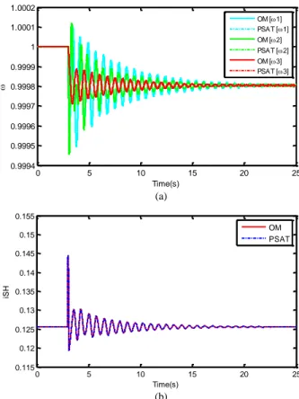
From the figures (8)-(11) it is obvious that Modelica and PSAT results have a satisfactory match. RMSE calculations also indicate that the results differences are within the tolerance range. Fig. 13 shows the time required to simulate the IEEE 9-Bus system including TCSC using different solvers. The average simulation time took in PSAT with six different tolerances is 608 s.

V. CONCLUSSIONS AND FUTURE WORK

The models simulated in two different software packages accurately predict the same dynamic behavior, so it cannot be said that one is better than other; rather the modeling community is free to choose the modeling language. The

results show that the Modelica language is capable of providing similar results of those of typical power system simulation tools for time-domain analysis, and thus, the added values of the Modelica language (model portability and accessibility, and a standardized modeling language) can be fully exploited for power system simulation.

The oscillation damper input has not tested for any of the models, in future work it will be shown how Modelica tools can be used for power system control design and its advantage over typical power system tools. This will be carried out using both averaged models and detailed switching models that will be implemented through equation based modeling in future.

(a)

(b)

Figure 8: Software-to-Software validation results with STATCOM (a) speed of all three generators (b) state variable of STATCOM.

0 5 10 15 20 25 0.9994 0.9995 0.9996 0.9997 0.9998 0.9999 1 1.0001 1.0002 Time(s)  OM [1] PSAT [1] OM [2] PSAT [2] OM [3] PSAT [3] 0 5 10 15 20 25 0.115 0.12 0.125 0.13 0.135 0.14 0.145 0.15 0.155 Time(s) iS H OM PSAT 0 5 10 15 20 25 -0.03 -0.02 -0.01 0 0.01 0.02 Time(s) x1 OM PSAT

Figure 9: Software-to-Software validation results with TCSC.

Figure 10: Software-to-Software validation results with SSSC.

Figure 11: Software-to-Software validation results with UPFC.

Figure 12: Comparison of different solvers of OpenModelica with Trapezoidal rule of PSAT.

Figure 13: Total simulation time spending for the solvers in OpenModelica with different tolerance.

VI. REFERENCES

[1] L. Vanfretti, W. Li, T. Bogodorova, and P. Panciatici, “Unambiguous power system dynamic modeling and simulation using Modelica tools," IEEE Power and Energy Society General Meeting (PES), July 2013.

[2] Federico Milano. Power system modelling and scripting. Springer, 2010.

[3] J. Mahseredjian, V. Dinavahi, and J. Martinez, “Simulation Tools for Electromagnetic Transients in Power Systems: Overview and Challenges,” IEEE Transactions on Power Delivery, vol.24, no.3, pp.1657–1669, 2009.

[4] L. Vanfretti, T. Bogodorova, and M. Baudette “A Modelica Power System Component Library for Model Validation and Parameter Identification,” 10th International Modelica Conference, Lund, Sweden, 2014.

[5] E. Lambert, X. Yang, and X. Legrand, “Is CIM suitable for deriving a portable data format for simulation tools?,” IEEE Power and Energy Society General Meeting, July 2011.

[6] Rogersten, R.; Vanfretti, L.; Wei Li; Lidong Zhang; Mitra, P., "A quantitative method for the assessment of VSC-HVdc controller simulations in EMT tools," Innovative Smart Grid Technologies Conference Europe (ISGT-Europe), 2014 IEEE PES , vol., no., pp.1,5, 12-15 Oct. 2014

[7] C. A. Cañizares and Z. T. Faur, “Advantages and disadvantages of using various computer tools in electrical engineering courses”, IEEE Trans. Educ., vol. 40, no. 3, pp. 166171, Aug. 1997.

[8] F. Milano, L. Vanfretti, and J.C. Morataya, “An Open Source Power System Virtual Laboratory: The PSAT Case and Experience,” IEEE Transactions on Education, vol. 51, no.1, pp.17-23, Feb. 2008. [9] C. A. Cañizares and F. Alvarado, UWPFLOW: Continuation and Direct

Methods to Locate Fold Bifurcations in AC/DC/FACTS Power Systems,2006.[Online]. Available:http://thunderbox.uwaterloo.ca/ [10] PSAT: Power System Analysis Toolbox. [Online] Available:

http://faraday1.ucd.ie/psat.html

[11] R.D. Zimmerman, and R.J. Thomas, “PowerWeb: a tool for evaluating economic and reliability impacts of electric power market designs,” IEEE PES Power Systems Conference and Exposition, pp.1562-1567 vol.3, 10-13 Oct. 2004.

[12] M. Larsson, “ObjectStab: An educational tool for power system stability studies,” IEEE Trans. Power Syst., vol. 19, no. 1, pp. 5663, Feb. 2004.

[13] T. Bogodorova, M. Sabate, G. Leon, L. Vanfretti, M. Halat, J.B. Heyberger, and P. Panciatici, “A modelica power system library for phasor time-domain simulation,” 2013 4th IEEE/PES Innovative Smart Grid Technologies Europe (ISGT EUROPE), 6-9 Oct. 2013.

[14] P. Fritzson, Introduction to Modeling and Simulation of Technical and Physical Systems with Modelica. Wiley-IEEE Press, 2011. ISBN: 978-1-118-01068-6.

[15] iTesla: Innovative Tools for Electrical System Security within Large Areas. [Online]. Available: http://www.itesla-project.eu/

[16] F. Milano, Power System Analysis Toolbox Documentation for PSAT. version 2.1.8, 2013. 0 5 10 15 20 25 -0.3 -0.2 -0.1 0 0.1 0.2 Time(s) x0 OM PSAT 0 5 10 15 20 25 5 6 7 8 9 10 11x 10 -3 Time(s) x2 OM PSAT 0 5 10 15 20 25 -0.04 -0.02 0 0.02 0.04 Time(s) vs OM PSAT 0 5 10 15 20 25 -0.02 -0.01 0 0.01 Time(s) v p i OM PSAT 0 5 10 15 20 25 0 0.05 0.1 0.15 0.2 Time(s) iq OM PSAT 0 5 10 15 20 25 7.956 7.957 7.958 7.959 7.96 7.961x 10 -3 Time(s) vq OM PSAT 0 5 10 15 20 25 -0.025 -0.02 -0.015 -0.01 -0.005 0 0.005 0.01 0.015 Time(s) x1 RungeKutta Trapezoidal Dassl Euler 9.2 9.4 9.6 9.8 8 8.5 9 9.5x 10 -3

1e-10 1e-08 1e-06 1e-05

100 101 102 103 Tolerance Ti m e Euler Trapezoidal RungeKutta Dassl