Are international stock markets correlated? : Comparing NIKKEI, Dow Jones and Dax in the periods 1991-2000 and 2001-2010

J

Ö N K Ö P I N G

I

N T E R N A T I O N A L

B

U S I N E S S

S

C H O O L

JÖ N KÖ P I N G U N IVER SITY

Are international stock markets correlated?

Comparing NIKKEI, Dow Jones and DAX in the periods 1991-2000 and 2001-2010

Bachelor thesis within: Economics Author: Yang Fan Supervisor: Professor Hubert Fromlet PhD candidate Erik Åsberg Jönköping May 2011

1

Bachelor’s Thesis in Economics

Title: Are International stock markets correlated?

Comparing NIKKEI, Dow Jones and DAX in the periods of 1991-2000 and 2001-2010

Author: Yang Fan

Tutor: Professor Hubert Fromlet

PhD candidate Erik Åsberg

Date: [2011-05]

Abstract

With the process of financial globalization, many thousands of stock traders and stock brokers endeavor to seek the best portfolio diversification. Ever since the emergence of stock exchanges, whether international stock/equity markets are correlated or not gener-ates more and more attention by investors. Based upon the augmented Dickey- Fuller (ADF) test and the error correction model (ECM), this paper tests the cointegration of three of the biggest stock exchanges in the world. Two periods, 1991-2000 and 2001-2010 are studied. The main finding is that there is no cointegration in the long run peri-od among the tested markets, but in short run Dow Jone Industiral Average (DJIA) will affect Deutscher Aktien- Indice (DAX) and Nikkei Heikin Kabuka, 225 (NIKKEI 225). Key words: Financial globalization, cointegration, ADF, ECM.

2

Table of Contents

1

Introduction ... 4

1.1 Background ... 4

1.2 Main findings ... 5

1.3 Purpose of the study ... 5

1.4 Literature review ... 5

2

Data collection ... 7

3

Indices... 8

4

Methodology ... 9

4.1 Testing for unit roots ... 9

4.2 Testing for high orders of integration ... 12

4.3 Testing for cointegration ... 12

4.4 Error Correction Models ... 13

4.5 Vector Autoregressive Models ... 14

4.6 Granger Causality... 16

5

Empirical results ... 17

5.1 The results of Unit root and high order of integration ... 17

5.2 The result of cointegration ... 19

5.3 Short term relationships between the indices and ECM ... 20

5.4 The result of vector Autoregressive Models ... 24

5.5 Granger causality result ... 27

6

Conclusion ... 30

3

Tables

Table 1 Unit root test results ... 17

Table 2 Cointegration test result ... 19

Table 3 Coefficients of the regression models (1991-2000) ... 20

Table 4 Coefficients of the regression models (2001-2010) ... 20

Table 5 Coefficients of the Error Correction Models (1991-2000) ... 22

Table 6 Coefficients of the Error Correction Models (2001-2010) ... 22

Table 7 VAR Residual Normality Tests (1991-2000) ... 25

Table 8 VAR Residual Normality Tests (2001-2010) ... 26

Table 9 Parwise Granger Causality Tests (1991-2000) ... 27

Table 10 Parwise Granger Causality Tests (2001-2010) ... 28

Appendix ... 35

Appendix 1 ... 35 Appendix 2 ... 35 Appendix 3 ... 36 Appendix 4 ... 37 Appendix 5 ... 38 Appendix 6 ... 39

4

1

Introduction

1.1

Background

Over the last two decades, there has been remarkable growth in international capital flows, in an environment of rapid change in global politics and technology. However, the majority of capital transactions have taken place between rich industrialized coun-tries. In 2003, there were gross financial transactions of over $6.4 trillion of which $5.4 trillion (84%) was between 24 industrialized countries and approximately $1.0 trillion (15%), between the 162 less-developed countries (LDCs) or economic territories. Cross-border capital flows have been expanding in a considerable speed, much faster than the world GDP and the trade growth rate. And most of these capital flows took place in developed areas.

At first glance, financial globalization has become a crucial trend of the world economy in the 21st century, mainly due to large capital flows. Furthermore, a closer examination reveals that financial globalization can be traced back to the Bretton Woods System in 1944 (Bordo & Eichengreen, 1993). A new global economy pattern was shaped after the meeting. Thanks to asset price and currency movements, international spillovers have been enhanced, which can be considered a positive effect of financial globalization. Meanwhile, financial globalization has created tremendous changes in direction and magnitude of net capital flows. The explicit way to globalize is the trading of financial assets due to its merits that

“nothing is beyond exchanging pieces of paper or making entries in electronic ledgers,

no movements of physical goods or of people are involved. No frontiers have to be crossed. The only barriers are national regulations” (Tobin ,1999).

With a financial perspective on the process of financial globalization, correlated interna-tional stock/equity markets becomes an especially interesting topic that has been exam-ined by many scholars and investors. For an investor, low international correlation across markets is the crux of global portfolio diversification. The combinations of do-mestic stock markets total portfolio risk cannot be reduced until the correlation across national markets is lower than expectation, since obviously no one wishes to sacrifice

5

their returns. I am interested in this topic due to personal experience of trading stocks in China and a great interest of international stock markets, and whether or not an investor should invests his assets in different stock markets.

1.2

Main findings

The main findings of this paper is that there is no cointegration between these three in-dices after testing the unit root by Augmented Dickey Fuller test in the long run, in the short run however, the results imply that the DJIA strongly affect the DAX and the NIKKEI 225 while the latter two do not affect each other.

1.3

Purpose of the study

There are many previous empirical studies on the area of integration and most of those works focus at identifying how the stock markets in different countries are interrelated. Converged examples can be found in the following literature reviews. The core of this paper is to test the cointegration among three biggest economies around the world in the 1990s and from 2001-2010 by testing for unit roots and cointegration as well as Vector Autregressive Models and Error Correction Models from time series course since all the data can be describe as time series data.

1.4

Literature review

The relationship between international equity markets is well documented in literature. Cheung and Lai (1995) investigate long run memory in international stock markets re-turns by taking USA，Australia, Austria, Belgium, Canada, Denmark, France, Germa-ny, Hong Kong, Italy, Japan, Netherlands, Norway, Singapore/Malaysia, Spain, Swe-den, Switzerland and the UK into consideration. Two tests for short term dependence and conditional heteroscedasticity are used: a modified rescaled rang test and a fraction-al differencing test. A previous paper can be traced back to 1989 when Meric&Gulser (1989) investigated seasonality in international stock market relationship and the return of international portfolio diversification. They use Box’s M statistical test to test the equality of the variance – covariance matrices of 17 countries. Their main conclusion is that investors can gain more from portfolio diversification across countries even if with-in a sole with-industry than across with-industries withwith-in countries. Another similar literature is

6

held by Chan, Gup & Pan (1997). They extend the previous research on intergration of international stock markets by involving 18 countries and covering a 32 year period from January 1961 to December 1992. Their studies gives the conclusion that the corre-lations among returns to national stock markets are surprisingly low, and that interna-tional elements play an important role, which indicates that there exists good diversifi-cation opportunities for investors. (Chan, Gup & Pan, 1997).

Bhargave, Bose and Dubofsky (1998) found out that there was a general increase in the correlation of foreign markets with the US market over the time period of 1960s to 1990s. However the world overall market is relatively low over the long run because of the Asia market which is less correlated with US market. Currency issues also plays an important role in international portfolio diversification. Morana and Beltratti (2002) es-timated the effect on Europe of the introduction of the euro by means of a GARCH model with a dummy variable. France, Germany, Spain, Italy, UK and USA were in-cluded in the sample. They found that investors are better off in diversifying their assets across European countries rather than within countries that have troubles in adapting to new rules and financial issues. (Morana & Beltratti, 2002).

Emerging markets also cannot be ignored. Gilmore and McManus (2005), using the market data of Czech Republic, Hungary and Poland make the conclusion that the cor-relation between US and these Central European countries is relatively low, which im-plies that there exists a diversification chance for US and German investors. Phylaktis & Ravazzolo (2005) researched stock market linkages among a group of Pacific-Basin countries with US and Japan by using an autoregressive (AR) and a moving average (MA) model. They also found linkages among these stock markets that give internation-al investors portfolio diversification opportunities by investing in majority of Pacific-Basin countries.

The remainder of this study is outlined as follows: Section 2 & 3 (Data collection and Indices) – these section will provide the collection of the data and some limitations as well as a brief description of the chosen indices. Section 4 (Methodology) – this section is a general introduction of econometric methodology applied in this paper, for instance, testing for unit roots and high orders of integration; cointegration; ECM; VAR and

7

Granger Causality. Section 5 (Empirical results) – in this part the author will analyze the results after computing the regression, searching for the cointegration between the three stock markets. Section 6 (Conclusion) – an overall conclusion of empirical results and some recommendations for investors and further studies.

2

Data collection

In this paper, daily data for three major stock indices were used: Dow Jones Industrial Average (DJIA), Nikkei 225 and DAX, over the time period from January 1st 1991 to December 30th 2010.The chosen countries are the biggest economies of their continent and engines of world economic growth. GDP,Export, Investment and Capital flows are the main factors in justifying the choice of countries. The data base employed in this paper stems from yahoo finance, each of the indices have missing values in a specific data while others do not. For example, stock exchanges may be suspended on different counties’ national day or statutory holidays like Christmas and New Year, national catastrophies like 9/11 in USA and earthquake in Japan may also close down the stock exchange. The missing values will cause an uneven number of observations, which may lead biased conclusion and result. So, one had to remove such data when all of its indice values were not observed to even out from the number of observations generally. It is entirely ambiguous whether these time series should be assumed as growing over time or not, even though GDP and prices are growing over time. Changes are being ma-nipulated due to different index calculation methods, also the enterprises stock involved in the indices are changing. If the index values can be observed in the long term, only the DJIA and DAX seem to be growing over the period of 1990s (see appendix 1). For most of the tests, it is really complicated to summarize a tendency over time, but after scrutinizing it does not affect test results.

8

3

Indices

Three stock prices provide mainstream of quantitive fundamentals in this paper. The se-lected indices represent stock prices of countries located in different continents --USA, Japan and Germany- in order to test whether there is a cointegration or other alternative types of relations among global stock markets. The reason for choosing these three countries can mainly explained by the amount of GDP, Import and export. These coun-tries are representative of world financial markets since they are the leading economies of the world economy. China was excluded from the chosen observation due to the im-maturity of the stock market even though it experience tremendous growth over the last decades.

The Dow Jones Industrial Average (DJIA) is the most well known stock index in USA. The stock selection is not controlled by quantitative rules, a stock is generally included only if the company has a renowned reputation, demonstrate sustained growth and at-tract a large number of investors. Even though critics like Ric Edelman (2003) argue that DJIA is not accurate and does not represent overall market performance, it is still the most widely recognized and cited of the stock market index.

The Nikkei Heikin Kabuka, 225 is commonly referred to as the Nikkei index, or Nikkei Stock average. It is a price-weighted index consisting of 225 prominent stocks on the Tokyo Stock Exchange. The Nikkei has been calculated since 1950 and its direction is considered an indicator of the state of the Japanese economy. Most analysts consider it the Japanese equivalent of the Dow Jones Industrial Average. The Nikkei 225 is the most widely quoted average of Japanese equities, formerly called Nikkei-Dow Jones Average.

Deutscher Aktien-Indice (DAX), is a German Stock Index. It is traded on the Frankfurt Stock Exchange which is the biggest stock exchange in Germany. DAX Measures the development of the 30 largest and best-performing companies on the German equities market and represents around 80% of the market capitalization in Germany.

9

4

Methodology

4.1

Testing for unit roots

There are different ways to test whether a test a series is stationary or nonstationary, according to Gujarati& Porter (2009)

“a stochastic process is said to be stationary if its mean and variance are constant over time and the value of the covariance between the two time periods depends on the dis-tance or gap or lag between the two time periods and not the actual time at which the covariance is computed.”

Non-stationarity will cause “spurious regression”. As examples of thus, some interest-ing conclusions have been made, for example: the number of churches in a town seems to be related to the number of bars; beer drinking in the USA and child mortality in Ja-pan. Unit root test has become widely popular over the several years. The most popular one which used in this paper is the Dickey- Fuller test (Dickey & Fuller 1979, Fuller 1976). The basic object of the test is to test the null hypothesis that ρ=1 in:

yt = ρyt-1 + ut (1)

Against another alternative ρ<1, where ρ is the parameter value, ut stands for a white

noise error term.

H0: the series contains at least one unit root H1: the series do not contain unit root (stationary)

However, the regression is usually tested in first differences:

yt = γyt-1 + ut

So that a test of ρ=1 is equivalent to a test of γ=0 for first difference (since ρ-1=γ). Then we have:

H0: γ=0 (series contains at least one unit root) H1: γ<0 (series does not contain unit root)

10

There are three different specifications for the Augmented Dickey- Fuller (ADF) test equation.

H0: ρ=1 (or γ=0) H1: ρ<1 (or γ<0)

Specification 1 (no constant and no trend)

ΔYt= γ Yt-1 + Σ βi ΔYt-i + t (2) ΔYt = (ρ – 1)Yt-1 + Σ βi ΔYt-i + t (3)

If we do not reject the null hypothesis H0: ρ=1 (or γ=0), we can conclude that it is a nonstationary process; if we reject the null hypothesis that γ=0, then we can conclude that the series is stationary

Specification 2 (with constant but no trend)

ΔYt = γ Yt-1 + α + Σ βi ΔYt-i + t (4) ΔYt = (ρ – 1) Yt-1 + α + Σ βi ΔYt-i + t (5)

The null and alternative hypothesis are the same as above. If we do not reject the null hypothesis: ρ=1 (or γ=0), we can conclude that it is a nonstationary process; if we reject the null hypothesis that γ=0, then we can conclude that the series is stationary

Specification 3 (with constant and with trend)

ΔYt = γ Yt-1 + α + βt + Σ βi ΔYt-i + t (6) ΔYt = (ρ – 1)Yt-1 + α + βt + Σ βi ΔYt-i + t (7)

11

As the same, the null and alternative hypotheses do not change. If we do not reject the null hypothesis: ρ=1 (or γ=0), we can conclude that it is a nonstationary process; if we reject the null hypothesis that γ=0, then we can conclude that the series is stationary. Note that Σ βi ΔYt-I stand for the augmentation lags which corrects for potential autocor-relation and omitted variable bias to some extent. In practice, the augmented Dickey- Fuller test (rather than the nonaugmented one) is used so that the errors are ensured to be uncorrelated.

The problem of determining the optimal number of lags of the dependent variables can be solved by applying the information criteria like AIC and SBC, and choosing the model with the lowest information criteria.

Unit root testing strategies is complicated for three reasons:

1. They do not exploit prior knowledge of the growth status of the time series. 2. They worry about the unrealistic outcomes

3. Mass-significance, they double or triple –test for unit roots.

Elder & Kennedy (2001) suggest a relatively simple strategy that reduces these compli-cations. The core of this strategy is whether “an intercept”, “an intercept with a time trend”, or “neither an intercept nor a time trend” should be included in the regression to conduct the unit- root test.

Case 1: yt is growing Case 2: yt is not growing

12

4.2

Testing for high orders of integration

If series are non-stationary, yt must be differenced d times before it becomes stationary,

then it is said to be integrated of order d. Write as yt I(d).

Thus, if yt  I (d) then dyt I (0). An I (0) series is a stationary series; an I (1) series

contains one unit root, e.g. yt = yt-1 + ut

If xt~I(0), then xt is obviously stationary (xt~I(0)); xt~I(1), then xt is nonstationary but the 1st difference Δxt is stationary (Δxt~I(0)); If xt~I(k), then xt, Δxt, Δ2xt, Δ3xt ,…, Δk-1xt are nonstationary but the kth difference Δkxt is stationary (Δkxt~I(0))

Consider the simple regression: yt=  yt-1 + ut

H0: =0 (integrated of order 1 or higher, that is, at least one unit root) H1: <0 (stationary process)

If H0 is rejected we can conclude that yt does not contain any unit roots; if H0 is not re-jected then if there only has 1 unit root is not known. So there is at least 1 unit root. yt can be ytI(1), ytI(2),…or ytI(k). In practice, the integration order 0, 1, and 2 are the

only relevant integration orders.

4.3

Testing for cointegration

Engle and Granger proposed testing for cointegration by using the Dickey- Fuller test to determine whether the disturbances in a regression contain a stochastic trend. (Murray, 2006). The Engle- Granger test contains two steps:

Step 1: Pre-test the variables for their order of integration using e.g. ADF or PP. In cotegration analysis it is a necessary but not sufficient condition that the variables are in-tegrated of the same order as motioned in 2.2

13

Step 2: Estimate the long- run equilibrium relationship. If the results of step 1 indicate that both Yt and Xt are I (1) [or that both are I (2)], the the next step is to estimate the long-run relationship in the form:

yt = β0 + β1 * xt + et (8)

In order to decide if the variables are actually cointegrated, the following regression is used (where e is the residuals of the above regression):

∆et = a1 * et-1 + εt (9)

Our model is possible to estimate in the long-run, and is not spurious. However, in the short-run there might be disequilibrium. Therefore, we estimate an Error Correction Model.

New critical values for the Engle- Granger cointegration test. A one- side test, will ex-hibit the following critical values:

P (w<-1.65) = 5% Normal distribution P (w<-2.86) = 5% Dickey- Fuller distribution P (w<-3.34) = 5% Engle- Granger/ Mckinnon (Enders ,2004)

4.4

Error Correction Models

The error correction mechanism (ECM) first used by Sargan(1984) and later popular-ized by Engle and Granger corrects for disequilibrium. An important theory, known as the Granger representation theorem, states that if two variables Y and X are cointegrat-ed, the relationship between the two can be expressed as ECM. (Gujarati, 2009)

Cointegration is a measure of the long-run mechanisms in a variable, while error correc-tion models are useful for representing the short run relacorrec-tionships between variables.

14

Shocks can move the long-run relationship off track. Thus, we are not always at equilib-rium. Nevertheless there is a tendency to move towards equilibequilib-rium.

We can use both short-run (first-difference) and long-run (levels or log levels) infor-mation in a model. This model in commonly called an Error Correction Model (ECM). If yt= c + bxt+ut is the original model, and yt and xt are cointegrated[CI (1,1)], then this will be a highly consistent estimate of the relationship in the long run.

However, in the short run an ECM must be estimated:

∆yt = α0 + α1 * ∆xt + α2 * ut-1 + εt (10)

Since the variables are estimated in first difference this is modeling the short- run dy-namics of the model. ut is the lagged residual from the original model, which corrects for deviations from equilibrium. It relates deviations from equilibrium to changes in the dependent variable.

4.5

Vector Autoregressive Models

VAR is a natural generalization of autoregressive models that was popularized by Sims(1980). It is in a sense a systems regression model i.e. there is more than one de-pendent variable. The simplest case is a bivariate VAR (k), (where “k“is the number of lags, and “bivariate” defines that we have two endogenous variables) 𝑌𝑡= 𝛽10+𝛽11𝑌𝑡−1+⋯+𝛽1𝑝𝑌𝑡−𝑝+𝛾11𝑋𝑡−1+⋯+𝛾1𝑝𝑋𝑡−𝑝+𝑢1 (11)

𝑋𝑡= 𝛽20+𝛽21𝑌𝑡−1+⋯+𝛽2𝑝𝑌𝑡−𝑝+𝛾21𝑋𝑡−1+⋯+𝛾2𝑝𝑋𝑡−𝑝+𝑢2 (12)

So VAR (1) can be expressed as y1t = β10+β11y1t-1 +α11y2t-1+u1t (13)

Y2t = β20+β21y2t-1 +α11y2t-1+u2t (14)

Advantages of VAR modelling:

1. Do not need to specify which variables are endogenous or exogenous – all are en-dogenous.

15

2. Allows the value of a variable to depend on more than just its own lags or combina-tions of the white noise terms, so more general than ARMA modeling

3. Provided that there are no contemporaneous terms (= variables with no lags) on the right hand side of the equations, we are simply use OLS separately on each equation. 4. Forecasts are often better than “traditional structural” models.

Disadvantages of VAR modeling:

1. The biggest practical challenge in VAR modeling is to choose the appropriate lag length. This is very difficult and it is easy to make a mistake.

2. VAR models are less suited for policy analysis because of its emphasis on forecast-ing.

3. Do we need to ensure all components of the VAR are stationary? This is a very complicated debate regarding VAR models. But the general recommendation by most practitioners is to take the first difference for I (1) variables. (Enders (2010)) To solve the biggest problem in VAR modeling, choosing the optimal lag length for a VAR seems imperative.

There are several approaches for selecting lag length. The most popular ones are “cross-equation restrictions” and “information criteria”.

Cross- equation restrictions are also called Likelihood Ratio Test, LRT. As in (unre-stricted) VAR modeling, each equation should have the same lag length. The variance- covariance matrix of residuals, is denoted as Σ. The likelihood ratio test for this joint hypothesis is given by

LR = T [log|Σr|- log|Σu|]

Where Σr is the variance- covariance matrix of the residuals for the restricted model, Σu is the variance – covariance matrix of residuals for the unrestricted VAR, and T is the sample size.

Multivariate versions of the information criteria are required to test for optimal lag length in VAR models. The most common ones are Akaike’s (1974) information (AIC), Schwarz’s (1978) Bayesian information criterion (SBIC) and the Hanna- Quinn infor-mation criterion (HQIC). The formulas are express as:

16

MAIC = log |Σ| + 2k’ / T

MSBIC = log |Σ| + (k’ / T)log(T)

MHQIC = log |Σ| + (2k’ / T)log((log(T))

Where T is the total sample size, Σ is the variance covariance matrix of the disturbance terms k’ is the total number if regressors in all equations, which will be equal to g2k + g

for g equations, each with k lags of the g variables, plus a constant term in each equa-tion. The values of the information criteria are constructed for 0, 1, lags (up to some pre-specified maximum). (Brooks (2008))

4.6

Granger Causality

“Although regression analysis deals with the dependence of one variable to other varia-bles, it does not necessarily imply causation.” (Gujarati & Porter, 2009) Granger (1969) introduced a causality concept that has become quite popular in the econometrics litera-ture. He states that if lagged values of y2 help in predicting current values of y1 in a forecast form lagged values of both y2 and y1, then y2 is said to Granger cause y1. (Lüt-kepohl ,2004)

Granger Causality tests seek to answer questions such as “does changes in y1 cause changes in y2?” if y1 causes y2, lags of y1 should be significant in the equation for y2. If this is the case, we say that y1 “Granger- causes” y2.

If y2 causes y1, lage of y2 should be significant in the equation for y1. If both the sets of lags are significant, there is “bi- directional causality”

17

5

Empirical results

5.1

The results of Unit root and high order of integration

First, to make sure that the entire chosen stock index value data series have a unit root, Augmented Dickey- Fuller test were applied. The chosen data was assumed represent-ing case 1 in the Elder & Kennday approach (yt is growing) for DJIA and DAX, case 2 (yt is not growing) for NIKKEI 225. Therefore, when running this test, a constant and linear trend was included. Even if a trend is not evident (which perhaps could be the case for Nikkei, looking at all of its values from 1991-2000 that displays no growth), the result of the test remains the same in all of the cases.

Table 1 Unit root test results ADF t-statistic (1991-2000) ADF t-statistic (2001-2010) P-value (1991-2000) P-value (2001-2010) DJIA -2.483870 -1.870999 0.3362 0.3463 Diff_ DJIA1 -47.22259 -53.3280 0.0000 0.0001 Nikkei -2.360073 -1.614728 0.1534 0.4749 Diff_ Nikkei -49.05534 -50.39254 0.0001 0.0001 DAX -2.100484 -1.409783 0.5447 0.5790 Diff_ DAX -47.65947 -22.96030 0.0000 0.0000 N0= 2332 for year 1991-2000 N1=2348 for year 2001-2010

According to the results in table 1, the p value of DJIA, DAX, NIKKEI was higher than the critical value at 5% significance level (ADF t-statistic value is low) in two different periods, so the null hypothesis that DJIA, DAX, NIKKEI 225 has a unit root cannot be rejected which indicates that each stock indice has a unit root.

18

In the next step, testing whether there is a unit root after taking the first differences of each data series provides a way to determine if all of the chosen data are integrated of the same order. As can be seen from the table above, with the low p value (and high t-value), for example, the t- statistic and p-value of Diff_ DJIA is -47.22 and 0.00 from 1991-2000; -53.33 and 0.0001 from 2001-2010. Then the null hypothesis that DJIA, NIKKEI 225 and DAX contain a unit root is rejected at 5% significance level for both time periods. Now the conclusion is quite obvious: DJIA is intergrated of order one (DJIA ~I(1)), since ΔDJIA~I(0); NIKKEI 225 is integrated of order one (NIKKEI 225 ~I(1)), since ΔNIKKEI 225~I(0); DAX is integrated of the order one (DAX ~I(1)), since ΔDAX~I(0).

19

5.2

The result of cointegration

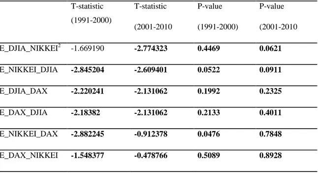
After making sure that all of the values of the chosen stock indices are integrated of the same order, we can test for cointegration by using the Engle- Granger methodology. The critical value for EG cointegration test is -3.350 (5% significance level and the ob-servations are over 500). Since the t-value of the test seem to vary a little bit depending on which was dependent variable in the equation that we acquired residuals, running the test on residuals that were required from equations that were run in both directions seems unbiased and appropriate.

Table 2 Cointegration test result T-statistic (1991-2000) T-statistic (2001-2010 P-value (1991-2000) P-value (2001-2010 E_DJIA_NIKKEI2 -1.669190 -2.774323 0.4469 0.0621 E_NIKKEI_DJIA -2.845204 -2.609401 0.0522 0.0911 E_DJIA_DAX -2.220241 -2.131062 0.1992 0.2325 E_DAX_DJIA -2.18382 -2.131062 0.2133 0.4011 E_NIKKEI_DAX -2.882245 -0.912378 0.0476 0.7848 E_DAX_NIKKEI -1.548377 -0.478766 0.5089 0.8928 N0= 2332 for year 1991-2000 N1= 2348 for year 2001-2010

All of the test results are compared with the 5% significance level of Engle- Granger ta-ble, which is -3.350. Since all of the Augmented Dickey- Fuller t-statistics in table 2 above has a value higher than -3.35, which can be seen from table 2. And therefore the residuals (et) like E_DJIA_NIKKEI; E_NIKKEI_DAX does contain a unit root. This means that DJIA; NIKKEI 225 and DAX are not cointegrated with each other (the null hypothesis that the residual of the regression between DJIA and NIKKEI 225 and DAX

20

have a unit root cannot be rejected). There is no cointegration between DJIA and NIKKEI and DAX.

5.3

Short term relationships between the indices and ECM

However, in the short-run there might be disequilibrium. The short term can be ex-plained by weekly effect or monthly effect among these three markets. Therefore, to avoid this problem, estimating an Error Correction Model is a good way to eliminate this problem.

All of the tests indicate no cointegration between indices. To learn more about short term relations between the indices, one way is running a regression on the first differ-ences of each data series:

∆Indice1(t) = α0 + α 1*∆Indice2(t) + e(t) (15) Table 3 Coefficients of the regression models (1991-2000)

D(DJIA) depend-ing on D(NIKK EI) D(DJIA) depend-ing on D(DAX) D(NIKKEI ) depending on D(DJIA) D(NIKKEI ) depeding on D(DAX) D(DAX) depend-ing on D(DJIA) D(DAX) depending on D(NIKKEI ) α0 3.638655 2.414511 -5.518550 -6.455465 1.111692 2.353528 α1 0.024911 0.515352 0.313177 0.944499 0.297652 0.043392 R2 0.007802 0.153396 0.007802 0.040983 0.153396 0.040983 N= 2332

Table 4 Coefficients of the regression models (2001-2010) D(DJIA) depend-ing on D(DJIA) depend-ing on D(NIKKEI ) depending D(NIKKEI ) depending D(DAX) depend-ing on D(DAX) depending on

21 D(NIKK EI) D(DAX) on D(DJIA) on D(DAX) D(DJIA) D(NIKKEI ) α0 0.342127 0.496053 -1.449218 -1.582127 0.343317 0.542721 α 1 -0.032598 -0.011090 -0.068492 0.811689 -0.000378 0.154447 R2 0.002233 0.000049 0.002233 0.125363 0.000049 0.125363 N= 2348

Judging from the coefficients it can be said that if the value change of DJIA increase by 1, the value change of NIKKEI will increase by 0.025, similarly, if the value changes if DJIA increase by 1, the value change of DAX will increase by 0.52, and so on. The α1 value suggests that there is positive correlation between values of stock indices in 1991-2000. But after step into 21st century, most of the α 1 values turns to be negative, the ex-ceptions comes from German stock market and Japan stock market, the data is 0.81 and 0.15, which means that when the value change of NIKKEI 225 increases by 1, the value change of DAX will increase by 0.81; on the other hand, if the value change of DAX increase by 1, the value change of NIKKEI 225 will increase by 0.15.

To remove the possible biases causes by shocks that affected only one of the equity markets, one need to estimate the Error Correction Models (ECM). The equation will be:

22

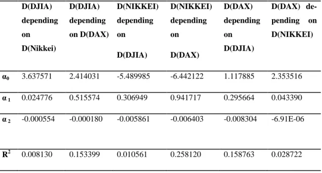
Table 5 Coefficients of the Error Correction Models (1991-2000)

D(DJIA) depending on D(Nikkei) D(DJIA) depending on D(DAX) D(NIKKEI) depending on D(DJIA) D(NIKKEI) depending on D(DAX) D(DAX) depending on D(DJIA) D(DAX) de-pending on D(NIKKEI) α0 3.637571 2.414031 -5.489985 -6.442122 1.117885 2.353516 α 1 0.024776 0.515574 0.306949 0.941717 0.295664 0.043390 α 2 -0.000554 -0.000180 -0.005861 -0.006403 -0.008304 -6.91E-06 R2 0.008130 0.153399 0.010561 0.258120 0.158763 0.028722 N= 2332

Table 6 Coefficients of the Error Correction Models (2001-2010) D(DJIA) depending on D(Nikkei) D(DJIA) depending on D(DAX) D(NIKKEI) depending on D(DJIA) D(NIKKEI) depending on D(DAX) D(DAX) depending on D(DJIA) D(DAX) depending on D(NIKKEI) α0 0.339608 0.495506 -1.434968 -1.577561 0.339237 0.540982 α 1 -0.029347 -0.003984 -0.063060 0.812852 -0.003354 0.154423 α 2 -0.009117 -0.005713 -0.010815 -0.002739 -0.013373 -0.002729 R2 0.005307 0.001297 0.009858 0.126232 0.014782 0.126407 N= 2348

α 2 usually referred to as the speed of adjustment coefficient. A large absolute value of α 2 is associated to a large value of D (NIKKEI) or D (DAX). However, if α 2 is zero, the changes in DJIA do not at all respond to the deviation from long- run equilibrium (t-1).

23

According to the theory, α 2 was expected to be negative, and it is true in this case. This implies that if NIKKEI 225 is above its equilibrium value, it will start falling in the next period to correct the equilibrium error; hence the name ECM. The absolute value de-scribes how quickly the equilibrium is restored.

Statistically, the equilibrium term is zero, suggesting that NIKKEI adjusts to change in DJIA in the same period. Short run changes in DJIA have positive impact on short- run changes in NIKKEI.

After comparing the tables containing information about simple regression and table containing information about the Error Correction Models, it is observed that the ECM models have a bit higher R-squared, but the coefficients are rather similar. This can be interpreted in a way that these stock markets are so well integrated that in the recent 20 years there has been no big shock which would have been contained in just one of the stock markets.

24

5.4

The result of vector Autoregressive Models

To find out more information about the short term relationships between the indices, the VAR model is utilized.

Since SC and HQ are the consistent criteria (the observations are over 2000), the small-est value is chosen upon criteria. It can be assumed that the optimal lag length for VAR could be 1 in this case from appendix 3.

As can be seen from the t-values, several coefficients seem to be insignificant (t-critical is 1.96 at 5% significance level). Only the first lag of differenced values of DJIA seems to be significant to determine the differenced values of DAX and NIKKEI. While the differenced values of Nikkei and DAX are significantly affected by the first lag of dif-ferenced DAX and NIKKEI values. See appendix 4. Meanwhile, all of these significant coefficients have a positive sign which is a good thing as it suggest that the past value of these stock indices are positively correlated with today’s value.

Since SC and HQ are consistent criteria (the observations are over 2000), the smallest values are chosen upon criteria. So it can be assumed that the optimal lag length for VAR could be 4 in this case. See appendix 5.

Apart from the points discussed from 1991-2000, the situation in 2001-2010 are com-plicated and difficult to interpret, in as much as there are plenty of insignificant lagged values. For example, the first and second lags of DAX are insignificant to the first dif-ferenced value of DJIA. However, like the situation in 1991-2000, all of these signifi-cant coefficients have a positive sign. See appendix 6.

Before interpreting the coefficients, the residuals of the model must be tested to make sure they are not white noise.

25

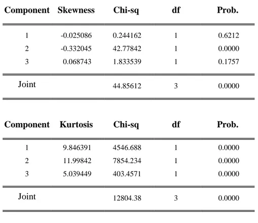
Table 7 VAR Residual Normality Tests (1991-2000)

Component Skewness Chi-sq df Prob.

1 -0.025086 0.244162 1 0.6212

2 -0.332045 42.77842 1 0.0000

3 0.068743 1.833539 1 0.1757

Joint 44.85612 3 0.0000

Component Kurtosis Chi-sq df Prob.

1 9.846391 4546.688 1 0.0000

2 11.99842 7854.234 1 0.0000

3 5.039449 403.4571 1 0.0000

Joint 12804.38 3 0.0000

Component Jarque-Bera df Prob.

1 4546.932 2 0.0000

2 7897.013 2 0.0000

3 405.2906 2 0.0000

Joint 12849.24 6 0.0000

N= 2332

H0: Normally distributed residuals H1: Not normally distributed residuals

Also the Granger causality between the difference values can be tested under the VAR model in table 8.

26

Table 8 VAR Residual Normality Tests (2001-2010)

Component Skewness Chi-sq df Prob.

1 -0.514793 103.1778 1 0.0000

2 -0.321907 40.34426 1 0.0000

3 -0.022972 0.205460 1 0.6503

Joint 143.7276 3 0.0000

Component Kurtosis Chi-sq df Prob.

1 8.899499 3387.598 1 0.0000

2 8.099018 2530.665 1 0.0000

3 5.706665 713.0675 1 0.0000

Joint 6631.331 3 0.0000

Component Jarque-Bera df Prob.

1 3490.776 2 0.0000

2 2571.010 2 0.0000

3 713.2729 2 0.0000

Joint 6775.058 6 0.0000

N= 2348

H0: Normally distributed residuals H1: Not normally distributed residuals

Since all of the p-values are 0.00 from table 7 and 8, we reject the null hypothesis which means that the residuals are not normally distributed. Therefore we can conclude that the residuals are not a white noise so this VAR model is bad and there is no use to inter-pret the values of the coefficients.

27

5.5

Granger causality result

One can also test the direction of the causality in the VAR model. Estimate a Granger causality test.

Table 9 Parwise Granger Causality Tests (1991-2000)

Null Hypothesis: Obs F-Statistic Prob.

DIFF_NIKKEI does not Granger Cause DIFF_DJIA 2329 1.00996 0.3150

DIFF_DJIA does not Granger Cause DIFF_NIKKEI 122.283 1.E-27

Null Hypothesis: Obs F-Statistic Prob.

DIFF_DAX does not Granger Cause

DIFF_DJIA 2329 0.82792 0.3630

DIFF_DJIA does not Granger Cause DIFF_DAX 217.338 4.E-47

Null Hypothesis: Obs F-Statistic Prob.

DIFF_DAX does not Granger Cause

DIFF_NIKKEI 2329 57.9105 4.E-14

DIFF_NIKKEI does not Granger Cause DIFF_DAX 9.16597 0.0025

5.5.1 5.5.2 5.5.3 5.5.4

N= 2332

Thus, since [p-value = 0.3150] > [0.05 = significance level] => we cannot reject H0 (see table 9). H0 is probably correct, that is, differenced value of Nikkei does not Granger Cause the differenced values of DJIA. This implies the stock indices change in Nikkei does not cause the change of DJIA.

28

On the other hand, in the lower part of the panel (Dependent variable: DIFF_NIKKEI), the following test hypothesis is tested:

H0: DIFF_DJIA does not Granger Cause DIFF_NIKKEI H1: DIFF_NIKKEI does not Granger Cause DIFF_DJIA

Thus, since [p-value = 1.E-27] < [0.05 = significance level] => H0 is rejected. H1 is probably correct, that is, differenced values of DJIA do Granger Cause differenced val-ues of Nikkei.

Similarly, differenced values of DJIA causes differenced value of DAX and also differ-enced values of DAX and the differdiffer-enced values of NIKKEI seems Granger cause each other.

Table 10 Parwise Granger Causality Tests (2001-2010)

Null Hypothesis: Obs F-Statistic Prob.

DIFF_NIKKEI does not Granger Cause DIFF_DJIA 2344 2.08911 0.1240

DIFF_DJIA does not Granger Cause DIFF_NIKKEI 334.050 2E-128

Null Hypothesis: Obs F-Statistic Prob.

DIFF_DAX does not Granger Cause

DIFF_DJIA 2340 0.34636 0.7073

DIFF_DJIA does not Granger Cause DIFF_DAX 884.243 1E-286

Null Hypothesis: Obs F-Statistic Prob.

DIFF_NIKKEI does not Granger Cause

DIFF_DAX 2340 0.71710 0.4883

DIFF_DAX does not Granger Cause DIFF_NIKKEI 185.322 2.E-75

29

Thus, since [p-value = 0.1240] > [0.05 = significance level] => cannot reject H0 (see ta-ble 10). H0 is probably correct, that is, differenced value of Nikkei does not Granger Cause the differenced values of DJIA. This implies the stock indices change in Nikkei does not cause the change of DJIA.

On the other hand, in the lower part of the panel (Dependent variable: DIFF_NIKKEI), the following test hypothesis is tested:

H0: DIFF_DJIA does not Granger Cause DIFF_NIKKEI H1: DIFF_NIKKEI does not Granger Cause DIFF_DJIA

Thus, since [p-value = 2.E-128] < [0.05 = significance level] => H0 is rejected. H1 is probably correct, that is, differenced values of DJIA do Granger Cause differenced val-ues of Nikkei. This is probably due to the large size of the US stock market. This im-plies that changes in DJIA will affect the NIKKEI 225 somehow from 2001-2010. Similarly, differenced values of DJIA causes differenced value of DAX and also differ-enced values of DAX Granger causes NIKKEI 225, NIKKEI 225 does not Granger cause DAX.

30

6

Conclusion

The key to succesful global portfolio diversification is expectations of low international correlation. This paper has used a Augmented Dickey- Fuller test to test unit roots first-ly and then cointegration over the long run. Error Correction models were used to re-move disequilibrium in the short run. The main finding of this paper is that there is no cointegration between these three indices, following that all of the time series contained a unit root and correlated of the same order. However, there is an evident short term re-lationship between all of the indices. The strongest one seems to be American DJIA af-fecting the German DAX (the effect of DJIA on DAX seems be the strongest from all of the explored relationships) and Nikkei 225. This outcome was expected and also sug-gested in previous researches by Bhargave (1998), Morana (2002) and Gillmore (2005). All of their primary result was that the correlation of the US and other countries were lower which clearly states that the US equity market is the most exogenous market in the world.

Also, the Granger causality suggests that in short term changes of DJIA value Granger causes changes in NIKKEI 225value and DAX value, also the changes in DAX value seems to be Granger causing changes in Nikkei 225 reciprocally in 1990s. Stepping into 21st century, the US equity market was still the dominating market in the world, which can be seen from the test results. Short term changes of DJIA value Granger causes changes in NIKKEI 225 and DAX values, NIKKEI 225 seems not Granger causes DAX while DAX still Granger causes NIKKEI 225.

The empirical results of ECM and the simple linear regression demonstrate that there have been no big shocks in the stock markets during the past 20 years. From 2000 until now, the worlds largest equity markets appear uncorrelated. All of these markets experi-enced a drop during 2001-2010 (see appendix 1 & 2), especially in 2008 when the glob-al financiglob-al crisis burst out, which means that there is a strong connection between the equity markets all over the world and most likely any significant failure of the financial system will have an effect on the equity markets all over the world. This also dimin-ished the possibilities to substantially lower the risk of the portfolio by engaging in transnational investing.

31

Overall, since stock markets do not have a long run comovement, It is possible for In-vestment banks, stock traders or any other investors to keep their assets from shrinking when having a cross border diversification investment instead of just single market in the long run.

Moreover, the author suggest further studies to explore and analyze the correlation be-tween stock markets and exchange rate from fixed rate regime to floating reate regime among different countries. Since the volatility of exchange rate also deem an important factor in influencing the international capital flow. (Christopher, 1990)

32

References

Bhargava, R; A. Bose & D.A. Dubofsky (1998). Exploiting international stock market correlations with opern- end international mutual funds. Journal of Business Finance &

Accounting, 25(5) & (6), June/July 1998, 0306- 686X

Bracher, K; D.S. Docking & P.D. Koch (1999). Economic determinants of evolution in international stock market integration. Journal of empirical finance 6, 1-27.

Bordo, M.D. & B. Eichengreen (1993). “A Retrospective on the Bretton Woods System:

Lessons for International Monetary Reform” University of Chicago Press, 1993.

Chan, K.C; B.E. Gup & M.S. Pan (1997). International Stock Market Efficiency and In-tergration: A study of eighteen nations. Journal of Business Finance & Accounting, 24 (6), July 1997, 0306- 686X.

Cheung, Y.W. & K.S. Lai (1995). A search for long memory in international stock mar-ket returns. Journal of Internaitonal Money and Finance, Vol. 14, No. 4, PP. 597-615, 1995.

Christopher K.M. & G. W. Kao (1990). On exchange rate changes and stock price reac-tions. Journal of Business Finance & Accounting, 17 (3) Summer 1990, 0306 686X. Dickey, D.A & W.A. Fuller (1979). Distribution of the Estimators for Autoregressive Time Series with a Unit Root. Journal of the American Statistical Association, 74, p. 427-431.

Edelman, R (2003). “The Truth About Money 3rd Edition” Harper Paperbacks. p. 126. December 23 ISBN 978-0060566586.

Elder, J & P.E. Kenedy (2000). F versus t tests for units roots. Working paper.

33

Gilmore, C.G; G.M. McManus & A. Tezel (2005). Portfolio allocations and the emerg-ing equity markets of Central Europe. Journal of Multinational Financail Management, 15 (2005) 287-300.

Grange, C.W.J (1969). Investing Causal Relations by Econometric Models and Cross- Spectral Methods. Econometrica,July 1969, PP. 424-428.

Gujarati, D.N & D.C. Porter (2009). “Basic Econometric”. 5th edition, Mc- Graw hill. Hill, R.C; W.E. Griffiths & G.C. Lim (2007). “Principles of econometrics” third edi-tion, Wiley.

Kouri, P.J.K & M.G. Porter (1974). International capital flows and portfolio equilibrium.

The Journal of political economy, Vol, 82. No.3. PP. 443-467

Lane, P.R & G.M.F. Milesi (2005) Financial globalization and exchange rate.

Interna-tional Monetary Fund.

Lütkepohl, H & M. Krätzig (2004). “Applied time series econometrics” Cambridge University Press.

Meric, I & G. Meric (1989). Potential gains from international portfolio diversification and inter-temporal stability and seasonality in international stock market relationships.

Journal of banking and finance 13, 627-640, north-holland.

Morana, C & A. Beltratti (2002). The effects of the introduction of the euros on the vol-atility of European stock markets. Journal of Banking & Finance 26, 2047-2064

Murray, M. P (2006). “Econometrics: a modern introduction” Pearson Addison Wesley. Phylaktis, K & F. Ravazzolo (2005). Stock market linkages in emerging markets: impli-cations for international portfolio diversification. Journal of International Financial

34

Sargan , J. D (1984). Wages and Prices in the United Kingdom: A study in Econometric Methodology, in K. F. Wallis and D. F. Hendry, eds. Quantitative Economics and

Econometric Analysis, Basil Blackwell, Oxford, U. K., 1984.

Sims, C. A (1980). Macroeconomics and Reality, Econometrica, vol. 48, pp. 1-48 Solnik, B; C. Boucrelle & Y. Lefur (1996). International market correlation and volatili-ty. Financial analysts jurnal.

Tobin, J (1999). Financial globalization. Cowles, foundation paper, No. 981.

Vincoop, E.V & T. Cedric (2007). International capital flows. National bureau of

eco-nomic research, working paper 12856.

Wei, S.J (2006). “International capital flows” prepared for the New Palgare dictionary of economics, second edition.

Wooldridge, J.M (2000). “Introductory econometrics: a modern approach” South- Western Cengage Learning.

Web sources http://www.djindices.com/ http://e.nikkei.com/e/fr/marketlive.aspx http://www.wikinvest.com/wiki/Nikkei_225 http://deutsche- bo-erse.com/dbag/dispatch/en/isg/gdb_navigation/private_investors/20_Equities/20_Indice s/10_DAX?module=InOverview_Indice&wp=DE0008469008&wplist=DE0008469008 &foldertype=_Indice http://www.econlib.org/library/Enc/InternationalCapitalFlows.html http://www.nber.org/papers/w12856 http://finance.yahoo.com/

35

Appendix

Appendix 1

The Overview of Historical Data of DJIA, NIKKEI & DAX from 1991-2000.

(1991-2000)

Appendix 2

The Overview of Historical Data of DJIA, NIKKEI & DAX from 2001-2010.

2,000 4,000 6,000 8,000 10,000 12,000 250 500 750 1000 1250 1500 1750 2000 2250 DJIA 12,000 14,000 16,000 18,000 20,000 22,000 24,000 26,000 28,000 250 500 750 1000 1250 1500 1750 2000 2250 NIKKEI 1,000 2,000 3,000 4,000 5,000 6,000 7,000 8,000 9,000 250 500 750 1000 1250 1500 1750 2000 2250 DAX

36

(2001-2010

Appendix 3

VAR Lag Order Selection Criteria output from 1991-2000.

Endogenous variables: DIFF_DAX DIFF_DJIA DIFF_NIKKEI

Lag LogL LR FPE AIC SC HQ

0 -42043.97 NA 1.07e+12 36.21617 36.22360 36.21888 1 -41875.33 336.6978 9.36e+11 36.07867 36.10838* 36.08950* 6,000 7,000 8,000 9,000 10,000 11,000 12,000 13,000 14,000 15,000 250 500 750 1000 1250 1500 1750 2000 2250 DJIA 6,000 8,000 10,000 12,000 14,000 16,000 18,000 20,000 250 500 750 1000 1250 1500 1750 2000 2250 NIKKEI 2,000 3,000 4,000 5,000 6,000 7,000 8,000 9,000 250 500 750 1000 1250 1500 1750 2000 2250 DAX

37 2 -41868.18 14.25881 9.38e+11 36.08026 36.13226 36.09921 3 -41860.88 14.53904 9.39e+11 36.08172 36.15601 36.10880 4 -41856.21 9.296872 9.43e+11 36.08545 36.18203 36.12064 5 -41836.36 39.41135 9.34e+11 36.07611 36.19498 36.11943 6 -41824.34 23.84987 9.31e+11 36.07351 36.21466 36.12494 7 -41820.01 8.578067 9.35e+11 36.07753 36.24097 36.13709 8 -41797.14 45.23777* 9.24e+11* 36.06559* 36.25131 36.13327 (1991-2000)

Appendix 4

Vector Autoregression Estimates output from 1991-2000. Standard errors in ( ) & t-statistics in [ ]

DIFF_DJIA DIFF_DAX DIFF_NIK KEI DIFF_DJIA(-1) 0.029232 0.242062 0.683085 (0.02254) (0.01635) (0.07767) [ 1.29693] [ 14.8044] [ 8.79416] DIFF_DAX(-1) -0.022262 -0.099447 0.391395 (0.03017) (0.02188) (0.10397) [-0.73790] [-4.54411] [ 3.76467] DIFF_NIKKEI(-1) -0.005088 -0.014318 -0.050503 (0.00597) (0.00433) (0.02057) [-0.85232] [-3.30618] [-2.45476]

38 C 3.470061 1.466517 -7.763563 (1.56445) (1.13487) (5.39129) [ 2.21808] [ 1.29223] [-1.44002] R-squared 0.001109 0.089864 0.055961 Adj. R-squared -0.000180 0.088690 0.054743

Appendix 5

VAR Lag Order Selection Criteria output from 2001-2010. Endogenous variables: DIFF_DAX DIFF_DJIA DIFF_NIKKEI

Lag LogL LR FPE AIC SC HQ

0 -43452.22 NA 3.28e+12 37.33267 37.34008 37.33537 1 -42721.93 1458.079 1.77e+12 36.71300 36.74265 36.72380 2 -42516.62 409.3780 1.49e+12 36.54435 36.59624 36.56326 3 -42481.72 69.51331 1.46e+12 36.52209 36.59623* 36.54911 4 -42450.64 61.81201 1.43e+12 36.50313 36.59950 36.53824* 5 -42441.06 19.03174 1.43e+12* 36.50263* 36.62124 36.54584 6 -42435.98 10.06950 1.44e+12 36.50600 36.64685 36.55732 7 -42432.24 7.410533 1.44e+12 36.51051 36.67361 36.56994 8 -42419.10 25.99959* 1.44e+12 36.50696 36.69229 36.57449

39

Appendix 6

Vector Autoregression Estimates Output from 2001-2010. Standard errors in ( ) & t-statistics in [ ]

DIFF_DAX DIFF_DJIA DIFF_NIKK EI DIFF_DAX(-1) -0.273482 -0.016312 0.382600 (0.02145) (0.04479) (0.05736) [-12.7486] [-0.36416] [ 6.66982] DIFF_DAX(-2) -0.119051 -0.046639 -0.018708 (0.02247) (0.04692) (0.06008) [-5.29839] [-0.99407] [-0.31137] DIFF_DAX(-3) -0.055045 0.176207 -0.063547 (0.02164) (0.04518) (0.05786) [-2.54379] [ 3.89978] [-1.09823] DIFF_DAX(-4) 0.010955 -0.169785 0.018411 (0.01809) (0.03777) (0.04837) [ 0.60561] [-4.49506] [ 0.38062]

40 DIFF_DJIA(-1) 0.400458 -0.087303 0.308881 (0.00991) (0.02069) (0.02650) [ 40.4152] [-4.21963] [ 11.6578] DIFF_DJIA(-2) 0.249970 -0.045560 0.528584 (0.01296) (0.02706) (0.03466) [ 19.2864] [-1.68348] [ 15.2515] DIFF_DJIA(-3) 0.104182 0.023678 0.117786 (0.01408) (0.02940) (0.03766) [ 7.39821] [ 0.80525] [ 3.12799] DIFF_DJIA(-4) 0.063881 -0.031605 0.111677 (0.01344) (0.02806) (0.03594) [ 4.75301] [-1.12618] [ 3.10740] DIFF_NIKKEI(-1) -0.004391 0.030387 -0.188110 (0.00803) (0.01676) (0.02147) [-0.54689] [ 1.81259] [-8.76190] DIFF_NIKKEI(-2) -0.010629 -0.015788 -0.044268 (0.00816) (0.01704) (0.02182) [-1.30238] [-0.92651] [-2.02852] DIFF_NIKKEI(-3) 0.004145 -0.025415 -0.022968 (0.00799) (0.01668) (0.02136) [ 0.51883] [-1.52351] [-1.07513] DIFF_NIKKEI(-4) 0.008204 -0.012657 -0.005969 (0.00735) (0.01534) (0.01965) [ 1.11672] [-0.82506] [-0.30384]

41 C 0.032945 0.555699 -2.106265 (1.25160) (2.61341) (3.34679) [ 0.02632] [ 0.21263] [-0.62934] R-squared 0.447819 0.037673 0.248953 Adj. R-squared 0.444967 0.032702 0.245073