Constructing an Index Fund Using Interior Point Primal- Dual Method

(1)

MASTER THESIS IN APPLIED MATHEMATICS

MMA891 Degree Project in Mathematics

Constructing an Index Fund Using Interior

Point Primal – Dual Method

by

Sampid Marius Galabe & Kamta Celestin

Masterarbete i matematik/tillämpad matematik

DIVISION OF APPLIED MATHEMATICS

MÄLARDALEN UNIVERSITY

(2)

Constructing an Index Fund Using Interior Point Primal – Dual Method

2

Master Thesis in Mathematics / Applied Mathematics Date: 2011-06-13

Project name: Constructing an Index Fund Using Interior Point Primal – Dual Method

Author:

Sampid Marius Galabe & Kamta Celestin

Supervisor: Dr. Kateryna Mishchenko. Examiner: Professor Anatoliy Malyarenko

(3)

3

Abstract

Optimization methods nowadays play a very important role in financial decisions such as portfolio managements, construction of index funds and pension funds.

This Master Thesis is devoted to the problem of an index fund construction. The problem is represented as a linear optimization problem of re-balancing the portfolio at minimum cost and solved using the Primal-Dual interior point method. The index fund is constructed using ten companies from the Dow Jones Industrial Average Index (DJIA).

(4)

4

Acknowledgement

We would like to give special thanks to our supervisor Dr. Kateryna Mishchenko for all her support and encouragement during the course of writing this thesis work. She has also been a great lecturer, teaching us very useful skills in programming languages. Also, special thanks to Dr. Torgil Abrahamsson and all our lectures at Mälardalens University, especially

(5)

Constructing an Index Fund Using Interior Point Primal – Dual Method 5 Table of Contents Definitions……….………...…...……….…...7 Introduction………..………....……….9 Background………...……...……….9 Method………...…...………9

i) Large scale deterministic model………...…………..………...……10

ii) Non linear programming model………....………11

iii) Linear programming model…...……….……...……...…12

Delimitation...…....12

Thesis overview...…...13

Chapter 1 Linear Programming Model…….……….……14

1.1 Derivation of the primal-dual method………..……….…….15

1.2 Sketch of the algorithm………...……..……….…………19

Chapter 2 Problem Modeling ………..……….…...21

Chapter 3 Implementation………..………...………..………27

3.1 Data collection………..………...………...27

3.2 The primal problem………...………..……28

3.3 The dual problem………..………..…....32

(6)

6

Chapter 4

The Java script………..………..……41 Conclusion………...……….………… …………..……….46 References………..….……….…....47 Appendix Java Code……….….………48 Applet Code………...…………...………75 Matlab Code………...……….107

(7)

7

Definitions

1. Bond: A bond is a debt security issued by institutions such as banks and governments for a period of more than one year in order to raise capital by borrowing. The bearer of the bond receives fixed interests at specific end dates. A pure discount bond makes just one payment of the principal amount and the interest at the end date while a coupon bearing bond makes several payments in the form of coupons over specific periods and payment of the principal amount at the end date.

2. Security: A security is an asset (financial instrument) other than an insurance policy issued by a government, a firm or any other financial organization which offers evidence of debt.

3. Stock: A stock or a share is a fraction of the ownership of a firm or business.

4. Expense ratio: This is the measure of how much it will cost an investment company to operate a mutual fund. This ratio “is determined through an annual calculation, where a fund’s operating expenses are divided by the average dollar value of its assets under management” [1].

5. Mutual fund: These are groups of investments such as stocks and bonds managed by a fund manager.

6. Market efficiency: This is the extent to which stock prices reflect all available information in the market.

7. Passive investments: These are investments characterized by restricted ongoing buying and selling actions in a well diversified portfolio, with the investors focusing on long term rather than short term profits [2].

8. Rebalancing: Rebalancing is the process of bringing a portfolio of investments that has deviated from the investor’s target asset allocation back to its original mix. This is done in order to control the amount of risk that the portfolio is exposed to.

9. Complementary slackness theorem: The complementary slackness theorem states that where are the optimal solutions to the primal problem and are the slacks of the dual problem.

10. Duality gap: This is the difference between the optimal objective function values of the primal and the dual problems.

11. Feasible set: A feasible set is a set of values that satisfy all constraints.

12. Convex set: Let C be a subset of C is said to be convex if for any two points a,b in C, the line segment joining a and b lies entirely in C.

(8)

8

13. Extreme points: Let C be a subset of If p is a boundary point of C, then p is called an extreme point if it has the following property: If any line segment lying entirely in C has p as one of its points, then p is an end point of .

14. Strictly feasible point: If is a strictly feasible point of the set then it satisfies the conditions .

15. Basic feasible solution: Basic feasible solution is any solution that arises at the extreme point of the feasible region. One of this solutions or a linear combination of this solutions will be the optimal solution.

(9)

9

Introduction

Background

An index fund is a portfolio intended to track the movement of the market as a whole or a given segment of the market. Tracking is done by trying to hold all the securities that constitute the index fund in the same proportion as the market index. Index funds are passive investments. They are also considered as a kind of mutual fund. Decisions concerning what securities are to be bought or sold are mostly carried out by computer programs with very little or no human effort.

Index funds have become very popular investments because of the following reasons: 1. Expense ratio; Index funds have lower expense ratios compared to conventional

mutual funds because they are passive investments and they generally give the advantage of lower fees and lower taxes in taxable accounts.

2. Empirical performance; top performing funds are not always consistent, which gives room for speculations that their performance are based on luck. However, the main idea behind an index fund is to build a portfolio of securities, such as stocks and bonds, designed to replicate as close as possible a well defined index.

3. Market efficiency; if the market is efficient, it will be impossible to obtain any superior risk adjusted return using stock picking strategies as a result of the fact that the prices reflect all the available information in the market. Also, “since the market portfolio provides the best possible return per unit of risk, to the extent that it captures the efficiency of the market via diversification, one may argue that the best theoretical approach to fund management is to invest in an index fund”[3]. This is because an index fund is designed to always try to replicate a specific market index.

Method

There exist several methods of constructing an index fund. A few examples are the large scale deterministic model, the non-linear programming model and the linear programming models.

(10)

10

i) Large scale deterministic model:

Large scale deterministic model separates a group of assets into smaller groups of similar assets and then selects representative asset from each group to be included in the index fund. The similarity between the stocks is determined by the correlation between their returns. The problem is formulated as a linear constraint maximization problem:

Subject to

In (1), is the correlation between stock i and j. In (2), q is the number of stocks in the

index fund, and if j is selected in the fund or 0 otherwise. (3) implies that each stock i has exactly one representative stock j in the index fund, and shows which stock j in the index fund is most similar to i. Thus, if j is the most similar stock in the index fund or

otherwise. (4) implies that stock i can be represented by stock j if and only if stock j is

in the fund [3].

The weights, , for each j in the fund are calculated as follows:

where is the current price of stock i, and the fraction of the index fund to be invested in stock j is given by:

(11)

11

where is the sum of all the different weights in the index fund and .

ii) Non-linear programming model

An example of creating an index fund using the non-linear programming model is to create an index fund from a portfolio of mutual funds [4]. First we need to determine the amount in percentage of the portfolio to be invested in each mutual fund that will closely replicate the performance of the market index. Suppose the portfolio consist of the following mutual funds:

A, B, C, D, E, and F, and let a, b, c, d, e, and f be the proportions invested in each of the

mutual funds respectively. Also, let be the portfolio return for year i, and be the return of the index in year i. Finally, let be the returns of A, B, C, D, E, and F in year i respectively. Then the portfolio returns for the five years period will be:

For each period, we compute the square of the deviations between the returns and the index. We square the deviations in order to avoid positive and negative deviations from cancelling out with each other thereby preventing a situation where portfolios with smaller values can behave quite differently than the target index. Thus we have the following optimization problem:

(12)

Constructing an Index Fund Using Interior Point Primal – Dual Method 12

The minimization problem is considered to be non-linear because of the presence of the quadratic term in the objective function.

iii) Linear programming (LP) model

LP model or linear optimization is one of the most common and fundamental problems developed as a mathematical model during World War II (1939) by Leonid Kantorovich. The model determines a way to achieve the best possible outcome with minimum cost. LP is “the problem of optimizing a linear objective function subject to linear equality and inequality constraints” [3].

Our objective is to construct an index fund that tracks a given segment of the market using the interior point method for linear programming.

Delimitations

The data used in this work was limited to daily data which we obtained from the Dow Jones website. We made several attempts to obtain monthly data including company details from three big indexes but our offers were turned down. Using daily data implies we have to be rebalancing our portfolio daily and this can be somehow expensive and time consuming. Also, since it was not possible to get inside information about company characteristics such as capitalization and payment of dividends, we grouped the companies together depending on the fraction of their weights in the index.

(13)

13

Thesis Overview

Chapter one discusses the LP model and briefly explains two successful techniques of solving LP problems. This chapter also describes the Primal-Dual interior point method in detail, which is the method we used in constructing an index fund. In Chapter two, we discuss the problem modeling and interpretation; we show the technique we used in selecting the various securities to constitute the index fund and how to set up the optimization problem.

In chapter three, we apply real data to the optimization problem formulated in chapter two and solve the problem using the Primal-Dual interior point method. This is followed by a

(14)

14

Chapter 1

Linear Programming Model

A Linear Programming (LP) problem has the standard form:

Subject to (11)

where _{; and x is the unknown variable vector to be determined,}

which is called the solution to the LP problem.

(11) is known as the Primal of the LP problem. The dual problem corresponding to problem (11) is:

Subject to (12)

The most successful technique for solving LP problems are the Simplex and the interior point methods.

The Simplex method solves an LP problem by use of extreme points. i.e.: it moves from one adjacent extreme point to the next. Thus, the Simplex method moves from one basic feasible solution to the next until the optimum is reached and operates on LP’s in standard form (see (11)).

Interior point methods are very efficient methods in linear optimization and have remarkable practical performance. The main feature of these methods is that iterates are strictly feasible. i.e.: they lie in the interior of the inequality constraints [5].

(15)

15

There are three main classes of interior point algorithms for linear programming and each of these algorithms are constructed by the means of the logarithmic barrier function [6]. These are the path-following methods, potential reduction methods and the affine scaling methods. The algorithms can be differentiated as either primal methods which maintains the feasibility of the primal, dual methods which maintains the feasibility of the dual or primal-dual methods which maintains the feasibility of both the primal and the dual.

We used the Primal-Dual methods in solving the optimization problems which arose from the construction of the index fund because this method over the years has proven to be the most efficient for solving LP problems.

1.1 Derivation of the Primal-Dual method

The primal problem can be stated in standard form as follow:

The dual problem can be stated in standard form as follow:

where are dual slack variables.

If is an iterate of the primal interior point method, then it satisfies the condition

, with and if is an iterate of the dual interior point methods,

then it satisfies the condition:

with .

(16)

16

Primal methods compute some estimates of the dual variables and dual methods also compute some estimates of the primal variables. For the case of the primal methods, convergence is achieved when the estimate for the dual is dual feasible and the duality gap within a specified tolerance is zero. Similarly, convergence can be obtained from the dual when the estimate for the primal is primal feasible and the duality gap within a specified tolerance is zero.

The Primal-Dual methods solve simultaneously, both the primal and the dual problems. The equality constraints on both the primal and dual are satisfied exactly while the non negativity constraints on and are strictly satisfied. When the duality gap is sufficiently small, meaning that convergence is attained, the algorithm terminates. Suppose is a feasible point to the primal and is a feasible point to the dual, then the following condition can be written on the duality gap [6]:

This condition is equivalent to the condition on complementary slackness.

Let’s consider the equations (P) and (D) above. A is assumed to be an matrix with full row rank while is an nxm matrix with full column rank and denotes the vector of dual slack variables. Let a feasible solution to (P) and (D) be and ( ) respectively. For these points to be optimal to (P) and (D), they must satisfy the complementary slackness conditions:

where n is the number of decision variables in the primal. This is same as number of constraints in the dual problem (D). The Primal-Dual method seeks to go through a chain of strictly feasible primal and dual iterates that get more and more closer to satisfying the complementary slackness conditions above.

For some parameter , each iteration seeks to find some vectors ) ) and ) Satisfying [6]

(17)

17

This process is repeated continuously with a reduction in the value of until convergence is attained within a specified tolerance. The strict feasibility of the iterates and s, i.e.: and s is guaranteed by the condition where . The duality gap is also constrained by these conditions. i.e.:

This implies that the sequence of primal-dual solutions produced by this algorithm will have decreasing duality gaps. The size of the duality gap determines the closeness to the solution. The points would be optimal if the duality gap were zero.

The complementary slackness condition can be written as

where

X=diag( ) is a diagonal matrix with diagonal term ,

S= diag( is a diagonal matrix with diagonal term ,

be the vector whose entries are all equal to one and with length . can equally be represented as follows:

The following derivations can be used to obtain an iterative scheme for estimates of the solution to (PD) [6].

If we assume that we have the following estimates: Such that

and that must not necessarily be equals to ; then the new estimates closest enough to satisfy these conditions are:

(18)

18

The primal and dual feasibility conditions would be:

and

These are systems of linear equations in with complementary slackness: An approximate solution is obtained by ignoring the product because are very small and hence is their product. Therefore, we have as the resulting system of equations: We have so far approximated a system of nonlinear equations by a system of linear equations by using the Newton’s method. The search direction for solving (PD) by performing one iteration of the Newton’s method at each iteration of the Primal-Dual method is known as the Newton direction.

Let are obtained by solving the system of linear equations:

(19)

Constructing an Index Fund Using Interior Point Primal – Dual Method 19 From (30), Multiply (31) by

Now, we define the diagonal matrix D as:

and let

then solution to (28), (29) and (30) above becomes:

and

1.2 Sketch of the Numerical Algorithm

With the rapid decrease in the solution might no longer be strictly feasible as required ( would no longer be satisfied). Thus we need to update current estimates as follows [6]:

(20)

Constructing an Index Fund Using Interior Point Primal – Dual Method 20 with

The largest step length is selected such that and are strictly positive and satisfying the following conditions [6]:

where and

(21)

21

Chapter 2 Problem modeling

We have n companies from which we want to select companies that would constitute an index fund. Each company represents an asset, therefore the number of assets equals n. We also have m characteristics that we would like the index fund to track. We have chosen four important characteristics; i.e.: m = A, B, C and D, where:

1. 2. 3.

4. If there are p, q, r, and s companies that belong to A, B, C, and D respectively; then the fraction of assets that belong to companies with small, medium and large capitalizations, and companies that pay dividends are respectively [7]:

The optimal weights are:

This means that:

Similarly:

(22)

22

If company 1 possesses characteristic A, then

And thus: Let:

The main idea of the derivation of the LP model for index fund construction is based on rebalancing of the portfolio at minimum cost. i.e.: maintain the portfolio’s risk closer to the investor’s level of risk tolerance. Some investments that do well in a portfolio usually take up more of the portfolio while those that do not do well usually take up less of the portfolio. This will make the portfolio become too risky or too conservative.

A very risky portfolio will earn more returns for the investor on a long term basis while on a short term basis, it might cause the investor great loses. If the portfolio is too conservative, the short term risk is reduced but the long term return is also lower. Therefore it is always

desirable to keep the portfolio at the investor’s preferred level of risk exposure. Therefore the problem formulation is as follows:

(23)

Constructing an Index Fund Using Interior Point Primal – Dual Method 23 Subject to: where (49) and (50) are defined as in (47) and (45) respectively.

(51) and (52) corresponds to constraints on the fractions bought and sold. Writing (51) and (52) in standard form gives:

where

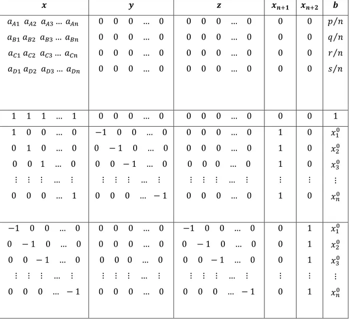
In order to easily formulate the dual of the above problem, we first of all transform the optimization problem above to blocks of matrices. Therefore the primal blocks can be written as follows:

(24)

Constructing an Index Fund Using Interior Point Primal – Dual Method 24 Table 1

Table represents constraints of primal problem.

From the above blocks, Table 1, the dual to the optimization problem with slack variables added can easily be constructed as follows:

Subject to:

(25)

Constructing an Index Fund Using Interior Point Primal – Dual Method 25 Where:

(26)

26 The constraints of the dual take the form:

where is a matrix of coefficients of w, s is a column matrix of coefficients of the slack variables, and c is a column matrix of coefficients of the primal objective function variables.

(27)

27

Chapter 3 Implementation 3.1 Data Collection

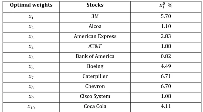
To implement the Primal-Dual method explained above, we used real data from the Dow Jones Industrial Average Index. For simplicity, we selected ten stocks to construct an index fund and all the ten stocks selected constitute the index fund. The selected stocks and their respective weights for the 15th of April are seen in the table below:

Table 4 Table 1

Table showing Stocks and respective weights for the 15th of April.

Now, we choose four characteristics that we want the index fund to track. We choose these characteristics based on their initial weights. i.e.: stocks with initial weights from 0.1% to 2% posses characteristics A, stocks with initial weights from 2.1% to 4% posses characteristics B, stocks with initial weights from 4.1% to 6% posses characteristics C, and stocks with initial weights from 6.1% to 8% posses characteristics D as seen in Table 5:

(28)

Grouping of stocks based on their initial weights.

The fractions of stocks with various characteristics are:

Let the optimal weights of the stocks be:

3.2 The Primal Problem

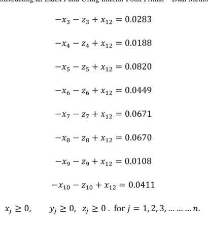
Minimization problem (48)evaluated by data introduced in Chapter 3.1, has the form:

Subject to:

(29)

29

This formulation can be rewritten as:

Subject to

(30)

The above constraints are the system of linear equations which should be solved to obtain an initial set of strictly feasible points with assumption that the fraction bought and fraction sold are given. One solution of this system is shown in the Table 6 below: Table 6 Table showing Initial set of strictly feasible points

(31)

31

The above constraints of the primal problem can also be represented in a matrix form so as to easily formulate the dual as follows:

Table 7

(32)

32

Table showing Block of matrices of the primal problem.

3.3 The Dual Problem

Now, taking the dual of (57), we have:

Subject to:

(33)

The initial set of feasible solution was obtained by solving the above system of linear equations. One of possible solutions is shown in Table 8 below:

(34)

Table showing Initial set of strictly feasible points

The entries of table 6 are entries of a 32 x 1 matrix, where the first entries are those of followed by The entries of table 8 constitute two matrices; 25 x 1 and 32 x 1. That is, w and s respectively. These are the initial set of strictly feasible points:

(35)

From starting from 10, we calculated the first iteration of the Primal – Dual method as follows:

We then computed:

For subsequent iterations, we reduced by dividing the preceding by 10 until the duality gap reached a certain tolerance (defined by the user). We then varied the tolerance to see its

(36)

36

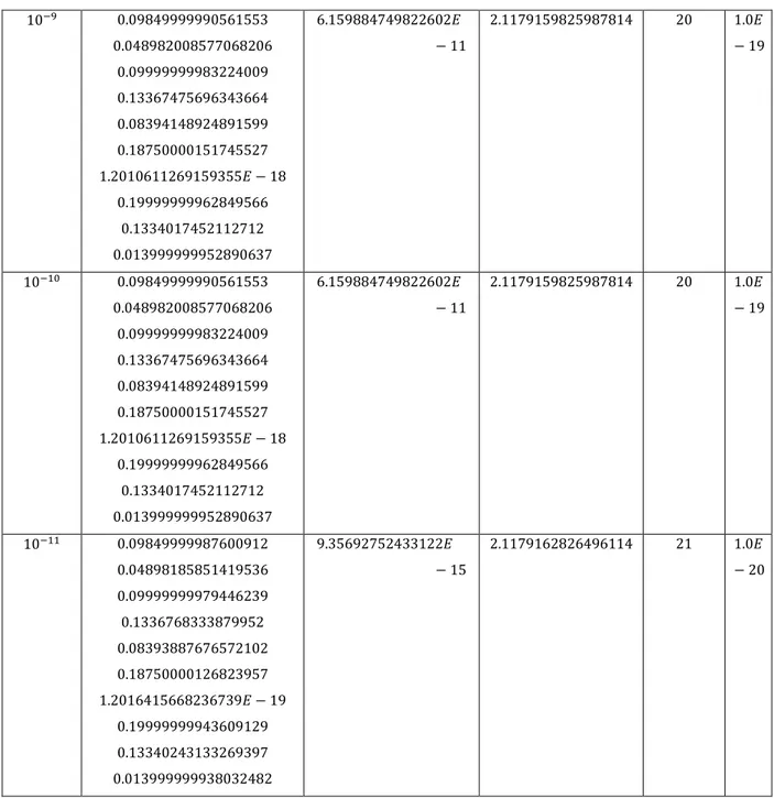
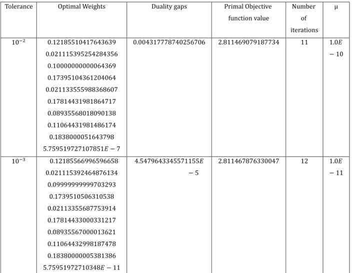
effect on the weights and observed that the weights changes with changes in tolerance as seen in Table 9 below. Table 9

(37)

(38)

Table showing Tolerance, Optimal weights, Duality gaps, Primal objective function value, Number of iterations and

3.4 Financial interpretation of results

It is observed that decrease in yields a decrease in objective function value and vice versa. measures how close the duality gap is to zero since the objective is to make the duality gap as close to zero as possible. is the risk and the smaller the more risk averse an investor is and vice versa.

(39)

39

The objective function value is the return and the more risk an investor is willing to take the greater the expected return and the more risk averse an investor is the smaller the expected return.

Note, however, that the problem is formulated as a minimization problem (minimizing fraction bought and sold), therefore with decreasing implies more risk aversion and hence a smaller objective function value.

Notice that same optimal weights are observed from a tolerance of _to _{with same}

value of ( and also from a tolerance of _to _{with same value of}

i.e.: the same risk for different tolerance yield the same expected return.

Varying y and z in (57)

Now, with variations in amounts bought and sold, the following results are obtained:

Table 10 Table showing variations in amounts bought and sold.

(40)

(41)

41

Chapter 4 The Java Script

The java package consists of a class called “matrixOperation” and a main class called “InteriorPm”.

In the class, we defined nine methods:

1. “matrixDiagonal” that computes a diagonal matrix from a vector. 2. “matrixmultiplication” that computes the product of two matrices. 3. “matrixsubtraction” that computes the difference of two matrices. 4. matrixaddition” that computes the sum of two matrices.

5. “matrixtranspose” that computes the transpose of a matrix. 6. “matrixinverse” that computes the inverse of a matrix.

7. “matrixScalamulti” that computes the product of a matrix and a scalar. 8. “printMatrix” that displays a matrix.

9. “ratio_test” that computes

NB. The code for “matrixinverse” was taken from the internet and uses Gaussian elimination for computing the inverse of a matrix [8].

The main class consists of matrix A, e, s, initial set of feasible solutions, x and w, from the primal problem and the dual problem respectively. e, s, x, w are all defined as matrices. We then designed an applet with tolerance as an input parameter and outputs parameters: objective function value, number of iterations, Mu and optimal weights as seen in Fig 1 below:

(42)

42

Fig 1

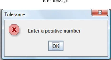
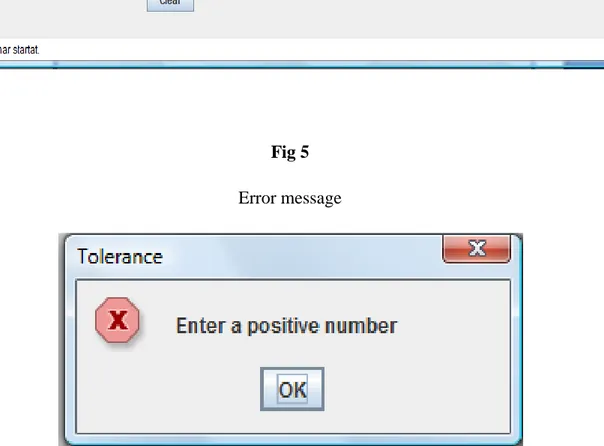
The applet is constructed in such a way that you can only enter a positive tolerance. If a wrong value is input i.e.: a negative number or any other character, then an error message will pop up reminding the user to input the proper value.

Also, the user is not allowed to edit in any other text field other than that for the tolerance. See Fig 2, 3, 4, 6, and 7 below:

(43)

43

Fig2

(44)

44

Fig 2

Non positive tolerance entered

Fig 3

(45)

45

Fig 4

Characters other than a positive number entered for tolerance

Fig 5

(46)

46

Conclusion

In this paper, we have constructed an index fund using sample companies and daily data from the Dow Jones Industrial Average Index. The problem was modeled as a portfolio rebalancing problem.

The primal problem was formulated from which the dual was obtained. Initial feasible solutions for both the primal and the dual were calculated manually and the problem was solved using the Primal-Dual interior point method.

The optimal weights that are obtained indicate the fraction of an investor’s wealth that can be invested in the corresponding companies in the index fund. This investment will yield a return that will be close to the market return indicated by the Dow Jones Industrial Average Index for that day. These optimal weights are the new weights in the investor’s rebalanced portfolio and since these weights were obtained by solving a minimization problem, it implies that we have obtained a rebalanced portfolio at minimum cost.

In both the Matlab and Java scripts, the initial feasible solutions were calculated manually and the number of companies used was limited to ten which yielded many constraint equations for both primal and dual problems. With more companies more constraints equations are

obtained, which are difficult to handle manually. However, with the use of more sophisticated software, it is possible to easily calculate initial feasible solutions and also include more than ten companies in the index fund.

(47)

47

References

[1] Investopedia. 2011. Expense Ratio. January 15 2011. <http://www.investopedia.com/terms/e/expenseratio.asp>

[2] Elton, Edwin J. et al. Modern Portfolio Theory and Investment Analysis. John Wiley & Sons 2007.

[3] Cornuejols, Gerard & Tutuncu, Reha, Optimization Methods in Finance. Cambridge University Press UK 2009.

[4] Anderson, R David. et al. An Introduction to Management Science: Quantitative Approaches to Decision Making, 12e. Thomson Corporation USA 2008.

[5] Igor Griva. et al. Linear and Nonlinear Optimization. Second Edition SIAM 2009 [6] Jorge Nocedal, Stephen J. Wright, Numerical Optimization.Second Edition Springer Science & Business Media, LLC 2006.

[7] Nigel, Meade and Salkin, Gerald R, Index Funds – Construction and Performance Measurement. The Management School, Imperial College, London. Journal of the Operational Research Society Vol. 40, No. 10, 1989.

[8] Java code for matrix inverse.

<http://www.daniweb.com/software-development/java/threads/118289>

[9] Brandimarte, P. Numerical Methods in Finance: A Matlab – Based Introduction. A Wiley-Interscience Publication 2006.

(48)

Constructing an Index Fund Using Interior Point Primal – Dual Method 48 Appendix Java Code // Class matrixOperation: /*

* To change this template, choose Tools | Templates * and open the template in the editor.

*/

/** *

* @author marius */

public class matrixOperation { double s[][];

static int i=0,j=0; double invS,diagx;

public static double[][] matrixDiagonal(double a[]){ int n = a.length;

double diag[][]=new double [n][n];// initialising array for( i=0;i<n;i++)

{

for (j = 0; j < n; j++) {

(49)

Constructing an Index Fund Using Interior Point Primal – Dual Method 49 diag[i][j] = 0; if(i==j){ diag[i][j]=a[i]; } System.out.print(diag[i][j]); } System.out.println(); } return diag; }

public static void printMatrix(double a[][]) {

int n=a.length; int m =a[0].length; for (int ii=0; ii<n; ++ii) for ( int h = 0; h<m; h++) { System.out.print(a[ii][h] + " "); } System.out.println(); }

(50)

50 {

int n=a.length; int m=a[0].length;

double A_sc[][]= new double[n][m];// initialising the array. //double c=1; for(int i=0;i<n;i++) for( int j=0;j<m;j++) A_sc[i][j] =b*a[i][j]; return A_sc; }

public static double[][] matrixaddition(double a[][],double b[][]) { int k1,k2= 0;

k1 = a.length; k2= b[0].length;

double sum[][]=new double[k1][k2]; for( int i=0;i<k1;i++)

{

for (int j = 0; j < k2; j++) {

sum[i][j] = a[i][j] + b[i][j]; System.out.print(sum[i][j]); }

(51)

51 }

return sum; }

public static double[][] matrixsubtraction(double a[][],double b[][]) { int k1,k2= 0;

k1 = a.length; k2= a[0].length;

double diff[][]=new double[k1][k2]; for( int i=0;i<k1;i++)

{

for (int j = 0; j < k2; j++) {

diff[i][j] = a[i][j] - b[i][j]; System.out.print(diff[i][j]+" "); } System.out.println(); } return diff; }

public static double[][] matrixtranspose(double a[][]) { int k1,k2=0;

(52)

52 k2= a[0].length;

double A_tr[][]= new double [k2][k1];// initialising array for( i=0;i<k2;i++) { for (j = 0; j < k1; j++) { A_tr[i][j] = a[j][i]; System.out.print(A_tr[i][j] + " "); } System.out.println(); } return A_tr; }

public static double ratio_test(double x[], double delta[]) {

int n=delta.length; double alpha;

double ratio[]= new double[n]; for(i=0;i<n;i++)

{

ratio[i] = 100000.0; if ( delta[i] < 0.0) {

(53)

Constructing an Index Fund Using Interior Point Primal – Dual Method 53 ratio[i] = -x[i]/delta[i]; j++; } } alpha = ratio[0]; for(i=1;i<n;i++) { if (ratio[i]<=alpha) alpha=ratio[i]; } return alpha; }

public static double[][] matrixmultiplication(double a[][], double b[][]) { int nn, mm, nk;

nn = a.length;//number of rows in matrix a

mm = b[0].length;//number of columns in matrix b nk = a[0].length; // number of columns in a

double product[][] = new double[nn][mm]; int k;

for (i=0; i<nn;i++) {

(54)

Constructing an Index Fund Using Interior Point Primal – Dual Method 54 { for (k = 0; k < nk; k++){ product[i][j]=product[i][j]+a[i][k]*b[k][j]; } System.out.print(product[i][j]+" "); } System.out.println(); } return product; }

// [8] reference to matrix inverse

public static double[][] matrixinverse(double a[][]){ int n=a.length;

double x[][] = new double[n][n]; double b[][] = new double[n][n]; int index[] = new int[n];

for (int i=0; i<n; ++i) b[i][i] = 1;

// Transform the matrix into an upper triangle gaussian(a, index);

// Update the matrix b[i][j] with the ratios stored for (int i=0; i<n-1; ++i)

(55)

55 for (int j=i+1; j<n; ++j)

for (int k=0; k<n; ++k) b[index[j]][k]

-= a[index[j]][i]*b[index[i]][k]; // Perform backward substitutions for (int i=0; i<n; ++i) {

x[n-1][i] = b[index[n-1]][i]/a[index[n-1]][n-1]; for (int j=n-2; j>=0; --j) { x[j][i] = b[index[j]][i]; for (int k=j+1; k<n; ++k) { x[j][i] -= a[index[j]][k]*x[k][i]; } x[j][i] /= a[index[j]][j]; } } return x; }

public static void gaussian(double a[][],int index[]) { int n = index.length;

double c[] = new double[n]; // Initialize the index

for (int i=0; i<n; ++i) index[i] = i;

(56)

56 for (int i=0; i<n; ++i) {

double c1 = 0; for (int j=0; j<n; ++j) { double c0 = Math.abs(a[i][j]); if (c0 > c1) c1 = c0; } c[i] = c1; }

// Search the pivoting element from each column int k = 0;

for (int j=0; j<n-1; ++j) { double pi1 = 0;

for (int i=j; i<n; ++i) {

double pi0 = Math.abs(a[index[i]][j]); pi0 /= c[index[i]]; if (pi0 > pi1) { pi1 = pi0; k = i; } }

// Interchange rows according to the pivoting order int itmp = index[j];

(57)

57 index[k] = itmp;

for (int i=j+1; i<n; ++i) {

double pj = a[index[i]][j]/a[index[j]][j]; // Record pivoting ratios below the diagonal a[index[i]][j] = pj;

// Modify other elements accordingly for (int l=j+1; l<n; ++l) a[index[i]][l] -= pj*a[index[j]][l]; } } } }

// Main Class InteriorPm: /*

* To change this template, choose Tools | Templates * and open the template in the editor.

*/

/** *

* @author marius */

(58)

58 public class InteriorPm {

/**

* @param args the command line arguments */

public static void main(String[] args) {

// double Duality_gap=100; // for(int i=0;i<15;i++){ // // // if(Duality_gap>Math.pow(10, -7)){ // u=Math.pow(10, -i); // }} double A[][]={{0, 1, 0, 1, 1, 0, 0, 0, 1, 0, 0, 0, 0 , 0 , 0 , 0 , 0 , 0 , 0 , 0 , 0 , 0 , 0 , 0 , 0 , 0 , 0 , 0 , 0 , 0 , 0 , 0}, {0 , 0 , 1 , 0 , 0 , 1 , 1 , 0 , 0 , 0 , 0, 0 , 0 , 0 , 0 , 0 , 0 , 0 , 0 , 0 , 0 , 0 , 0 , 0 , 0 , 0 , 0 , 0 , 0 , 0 , 0 , 0}, {1 , 0 , 0 , 0 , 0 , 1 , 0 , 0 , 0 , 1 , 0 , 0 , 0 , 0 , 0 , 0 , 0 , 0 , 0 , 0 , 0 , 0 , 0 , 0 , 0 , 0 , 0 , 0 , 0 , 0 , 0 , 0}, {0 , 0 , 0 , 0 , 0 , 0 , 1 , 1 , 0 , 0 , 0 , 0 , 0 , 0 , 0 , 0 , 0 , 0 , 0 , 0 , 0 , 0 , 0 , 0 , 0 , 0 , 0 , 0 , 0 , 0 , 0 , 0}, {1 , 1 , 1 , 1 , 1 , 1 , 1 , 1 , 1 , 1 , 0 , 0 , 0 , 0 , 0 , 0 , 0 , 0 , 0 , 0 , 0 , 0 ,0 , 0 , 0 , 0 , 0 , 0 , 0 , 0 , 0 , 0},

(59)

Constructing an Index Fund Using Interior Point Primal – Dual Method 59 {1 , 0 , 0 , 0 ,0 , 0 , 0 , 0 , 0 , 0 , -1 , 0 , 0 , 0 , 0 , 0 , 0 , 0 , 0 , 0 , -1 , 0 , 0 , 0 , 0 , 0 , 0 , 0 , 0 , 0 , 1 , 0}, {0 , 1 , 0 , 0 , 0 , 0 , 0 , 0 , 0 , 0 , 0 , -1 , 0 , 0 , 0 , 0 , 0 , 0 , 0 , 0 , 0 , -1 , 0 , 0 , 0 , 0 , 0 , 0 , 0 , 0 , 1 , 0}, {0 , 0 , 1 , 0 , 0 , 0 , 0 , 0 , 0 , 0 , 0 , 0 ,-1 , 0 , 0 , 0 , 0 , 0 , 0 , 0 , 0 , 0 , -1, 0 , 0 , 0, 0 , 0 , 0 , 0 , 1 , 0}, {0, 0, 0 , 1 , 0, 0 , 0, 0 , 0 , 0, 0 , 0 , 0 , -1 , 0 , 0 , 0 , 0 , 0, 0 , 0 , 0 , 0 , -1 , 0 , 0, 0 , 0 , 0 , 0 , 1 , 0}, {0 , 0 , 0 , 0 , 1 , 0 , 0 , 0 , 0 , 0 , 0, 0, 0, 0, -1 , 0, 0 , 0, 0, 0, 0 , 0, 0, 0, -1, 0, 0, 0 , 0, 0, 1 , 0}, {0 , 0 , 0, 0, 0, 1, 0, 0, 0, 0, 0, 0, 0, 0, 0, -1 , 0, 0, 0, 0 , 0, 0, 0, 0 , 0, -1, 0, 0, 0, 0, 1, 0}, {0 , 0, 0 , 0 , 0 , 0 , 1 , 0, 0, 0, 0, 0, 0, 0, 0, 0, -1, 0, 0, 0, 0, 0, 0, 0, 0, 0, -1 , 0, 0 , 0 , 1 , 0}, { 0 , 0 , 0 , 0, 0, 0, 0 , 1 , 0, 0, 0, 0, 0, 0, 0, 0, 0, -1 , 0, 0, 0, 0 , 0 , 0, 0, 0, 0 , -1, 0, 0, 1, 0}, {0 , 0 , 0 , 0 , 0 , 0 , 0 , 0 , 1 , 0, 0 , 0, 0 , 0 , 0, 0 , 0 , 0 , -1 , 0, 0 , 0 , 0 , 0 , 0, 0 , 0, 0, -1, 0 , 1 , 0}, {0 , 0, 0, 0 , 0 , 0 , 0 , 0 , 0 , 1 , 0 , 0 , 0 , 0 , 0 , 0 , 0 , 0 , 0 , -1 , 0 , 0 , 0 , 0 , 0 , 0 , 0 , 0 , 0 , --1 , -1 , 0}, {-1 , 0 , 0 , 0 , 0 , 0 , 0 , 0 , 0 , 0 , 0 , 0 , 0 , 0 , 0 , 0 , 0 , 0 , 0, 0 , -1, 0 , 0 , 0, 0, 0, 0 , 0 , 0 , 0 , 0, 1}, {0 , -1 , 0 , 0, 0, 0 , 0, 0, 0 , 0 , 0 , 0 , 0 , 0 , 0 , 0 , 0 , 0 , 0 , 0 , 0 , -1 , 0 , 0 , 0 , 0 , 0 , 0 , 0, 0 , 0 , 1}, {0 , 0 , -1 , 0 , 0 , 0 , 0 , 0 , 0 , 0 , 0 , 0 , 0 , 0 , 0 , 0, 0 , 0 , 0, 0 , 0 , 0 , -1 , 0 , 0 , 0 , 0 , 0 , 0 , 0 , 0, 1},

(60)

Constructing an Index Fund Using Interior Point Primal – Dual Method 60 {0 , 0 , 0 ,-1 , 0, 0 , 0, 0 , 0 , 0, 0, 0 , 0 , 0, 0 , 0 , 0 , 0 ,0 , 0 , 0 , 0 , 0 , -1 , 0 , 0 , 0 , 0 , 0 , 0 , 0, 1}, {0 , 0, 0 , 0 , -1, 0, 0 , 0, 0 , 0, 0 , 0, 0 , 0, 0 , 0 , 0 , 0 , 0 , 0, 0 , 0 , 0 , 0 , -1 , 0 , 0, 0, 0, 0 , 0, 1}, {0 , 0, 0, 0 , 0 , -1 , 0 , 0, 0, 0, 0, 0, 0, 0 , 0 , 0, 0, 0, 0 , 0, 0 , 0 , 0, 0 , 0 , -1 , 0, 0, 0 , 0, 0, 1}, {0 , 0 , 0 , 0 , 0 , 0, -1 , 0 , 0, 0 , 0, 0, 0 , 0, 0, 0, 0 , 0 , 0, 0, 0, 0, 0, 0 , 0 , 0, -1, 0, 0, 0, 0, 1}, {0 , 0, 0 , 0 , 0 , 0 , 0 , -1 , 0 , 0 , 0 , 0 , 0 , 0 , 0 , 0 , 0 , 0 , 0 , 0 , 0, 0 , 0 , 0, 0 , 0 , 0 , -1 , 0 , 0 , 0, 1}, {0 , 0, 0 , 0 , 0 , 0 , 0, 0 , -1 , 0 , 0 , 0 , 0 , 0, 0 , 0 , 0 , 0 , 0 , 0 , 0, 0 , 0 , 0 , 0, 0 , 0 , 0 , -1, 0, 0, 1}, {0 , 0, 0 , 0 , 0, 0 , 0 , 0, 0, -1 , 0 , 0 , 0 , 0 , 0 , 0 , 0 , 0 , 0 , 0, 0 , 0 , 0, 0 , 0, 0 , 0 , 0, 0 , -1, 0, 1}}; double s[][]= {{1}, {3}, {4}, {3}, {3}, {3}, {3}, {1}, {3}, {3}, {1}, {1}, {1}, {1}, {1}, {1}, {1}, {1}, {1}, {0.5}, {1}, {1}, {1}, {1}, {1}, {1}, {1}, {1}, {1}, {0.5}, {0.5}, {0.5}}; // double x[][] = {{0.00625}, { 0.025}, {0.1}, {0.0875}, {0.1375}, {0.16875}, // {0.01875}, {0.18125}, {0.15}, {0.125}, {0.2}, {0.5}, {0.14925}, {0.214}, {0.2717}, // {0.2687}, {0.2555}, {0.32385}, {0.15165}, {0.31425}, {0.3392}, {0.2839}, {0.43675}, // {0.464}, {0.3717}, {0.3937}, {0.2805}, {0.28635}, {0.41418}, {0.25175}, {0.3392}, {0.3339}}; // double x[][] = {{0.0125}, {0.05}, {0.1}, {0.15}, {0.025}, {0.2625}, {0.005},

(61)

Constructing an Index Fund Using Interior Point Primal – Dual Method 61 {0.195}, {0.175}, {0.025}, {0.1}, {0.4}, {0.0555}, {0.0139}, {0.1717}, {0.2312}, {0.043}, {0.3176}, {0.0379}, {0.228}, {0.2642}, {0.0839}, {0.3305}, {0.24}, {0.2717}, {0.3662}, {0.293}, {0.0926}, {0.03279}, {0.138}, {0.2142}, {0.3339}}; double w[][] = {{-1}, {-2}, {1}, {1}, {-2}, {0}, {0}, {0}, {0}, {0}, {0}, {0}, {0}, {0}, {-0.5}, {0}, {0}, {0}, {0}, {0}, {0}, {0}, {0}, {0}, {-0.5}}; double e[][]= {{1},{1}, {1}, {1}, {1}, {1}, {1}, {1}, {1}, {1}, {1}, {1}, {1}, {1}, {1}, {1}, {1}, {1}, {1}, {1}, {1}, {1}, {1}, {1}, {1}, {1}, {1}, {1}, {1}, {1}, {1}, {1}}; double x_tr[][],duality_gap[][], residual[][];

int counter;

double tol = 0.01;// input tolerance duality_gap = new double[1][1]; residual= new double[1][1]; double u =10; residual[0][0] = 100; double X[][],S[][]; double a_x[],a_s[]; int n= x.length; // int m= s.length;

//System.out.println(n); prints out the length of x. a_x = new double[n];

a_s = new double[m]; X = new double[n][n];

(62)

Constructing an Index Fund Using Interior Point Primal – Dual Method 62 S = new double[m][m]; //ue=new double[l][ln]; double D[][],invS[][]; D=new double [m][n]; invS=new double[m][m]; double XS[][], ue[][],v_u[][]; XS = new double[n][m]; duality_gap = residual;

double res = duality_gap[0][0]; // a scalar copy of matrix duality_gap

double Delta_w[][], Delta_x[][], AD[][],A_tr[][], ADA_tr[][], invADA_tr[][]; double invAD_A_tr_invS_vu[][], invADA_tr_A[][],invADA_tr_A_invS[][]; double Delta_s[][], A_tr_Delta_w[][],X_new[][],D_new[][],S_new[][]; double invS_v_u[][], D_Delta_s[][],invADA_tr_A_invS_v_u[][]; double alpha_p, alpha_d,Alpha_max, Ratio, XSe[][];

counter=0; int l = e.length; int ln=e[0].length; ue=new double[l][ln]; int ll = ue.length; int lnn=ue[0].length; v_u=new double[ll][lnn]; int m1=A.length; int m2=A[0].length;

(63)

63 AD= new double [m2][n];

ADA_tr=new double[m1][m1]; A_tr= new double[m2][m1]; invADA_tr= new double[m1][m1]; invADA_tr_A= new double[m1][m1]; invADA_tr_A_invS=new double [m1][m]; invADA_tr_A_invS_v_u= new double [m1][lnn]; int lll = invADA_tr_A_invS_v_u.length; int lnnn=invADA_tr_A_invS_v_u[0].length; Delta_w=new double[lll][lnnn]; A_tr_Delta_w=new double [m2][lnnn]; int llll = A_tr_Delta_w.length; int lnnnn=A_tr_Delta_w[0].length; Delta_s=new double[llll][lnnnn]; invS_v_u = new double[m][lnn]; D_Delta_s = new double[m][lnnnn]; Delta_x = new double[m][lnnnn]; double a_Delta_x[];//,a_s[];

int n1= Delta_x.length;

a_Delta_x = new double[n1]; double a_Delta_s[];//,a_s[]; int n2= Delta_s.length;

(64)

64 double Alpha_max_Delta_x[][], x_new[][]; int lllll = Delta_x.length;

int lnnnnn=Delta_x[0].length;

Alpha_max_Delta_x=new double[lllll][lnnnnn]; x_new=new double [lllll][lnnnnn];

double Alpha_max_Delta_w[][], w_new[][]; int llllll = Delta_w.length;

int lnnnnnn=Delta_w[0].length;

Alpha_max_Delta_w=new double[llllll][lnnnnnn]; w_new= new double[llllll][lnnnnnn];

double Alpha_max_Delta_s[][], s_new[][]; int lllllll,lnnnnnnn=0;

lllllll = Delta_s.length; lnnnnnnn=Delta_s[0].length;

Alpha_max_Delta_s=new double[lllllll][lnnnnnnn]; s_new= new double [m][m];

x_tr=new double[n][m];

while (Math.abs(duality_gap[0][0])> tol) {

counter++; System.out.println();

System.out.println("Number of Iteration = " + counter +". u = "+ u + "."); System.out.println();

(65)

Constructing an Index Fund Using Interior Point Primal – Dual Method 65 System.out.println("This is a_x "); for(int k=0;k<n;k++) { a_x[k] = x[k][0]; System.out.println(a_x[k]); } System.out.println(); System.out.println("This is a_s "); for(int k=0;k<m;k++) { a_s[k] = s[k][0]; System.out.println(a_s[k]); } System.out.println(); System.out.println("This is X ");

X=matrixOperation.matrixDiagonal(a_x);//input for matrix diagonal is x System.out.println();

System.out.println("This is S ");

S=matrixOperation.matrixDiagonal(a_s);//input for matrix diagonal is s System.out.println();

System.out.println("This is ue ");

ue =matrixOperation.matrixScalarMulti(e,u);// input matrices for //multiplication are u and e

(66)

Constructing an Index Fund Using Interior Point Primal – Dual Method 66 for(int i=0;i<l;i++) for(int j= 0;j<ln;j++){ System.out.println(ue[i][j]); } System.out.println(); System.out.println("This is XS ");

XS=matrixOperation.matrixmultiplication(X, S);//input matrices for //multiplication are X and S

System.out.println();

System.out.println("This is XSe ");

XSe=matrixOperation.matrixmultiplication(XS, e);//input matrices for //multiplication are XS and S

System.out.println("This is v_u ");

v_u= matrixOperation.matrixsubtraction(ue, XSe); System.out.println();

System.out.println(" This is invS "); System.out.println();

invS=matrixOperation.matrixinverse(S);//input for matrix inverse is S System.out.println();

System.out.println(" This is D ");

D=matrixOperation.matrixmultiplication(invS , X);// input matrices for //multiplication are invS and X

(67)

67 System.out.println();

System.out.println(" This is AD ");

AD= matrixOperation.matrixmultiplication(A, D);//input matrices for //multiplication are A and D

System.out.println(" This is A_tr ");

A_tr=matrixOperation.matrixtranspose(A);//input matrix for transpose A System.out.println();

System.out.println(" This is ADA_tr ");

ADA_tr= matrixOperation.matrixmultiplication(AD, A_tr);//input matrices for //multiplication are AD and AD_tr

System.out.println(" This is invADA_tr ");

invADA_tr=matrixOperation.matrixinverse(ADA_tr);//input matrices for //inverse is ADA_tr

System.out.println(" This is invADA_tr_A ");

invADA_tr_A=matrixOperation.matrixmultiplication(invADA_tr, A);//input //matrices

//for multiplicatiion are invADA_tr and A System.out.println();

(68)

68

invADA_tr_A_invS=matrixOperation.matrixmultiplication(invADA_tr_A, invS);//input //matrices for multiplicatiion

//are invADA_tr_A and invS System.out.println();

System.out.println(" This is invADA_tr_A_invS_v_u ");

invADA_tr_A_invS_v_u=matrixOperation.matrixmultiplication(invADA_tr_A_invS, v_u); //input matrices for multiplicatiion are invADA_tr_A_invS and v_u

System.out.println(" This is Delta_w");

Delta_w=matrixOperation.matrixScalarMulti(invADA_tr_A_invS_v_u, -1);//input //for matrix multiplicatiion

//is the scalar -1 and invADA_tr_A_invS_v_u for(int i=0;i<lll;i++) for(int j= 0;j<lnnn;j++){ System.out.println(Delta_w[i][j]+" "); } //calculation of Delta_s System.out.println();

System.out.println(" This is A_tr_Delta_w");

A_tr_Delta_w=matrixOperation.matrixmultiplication(A_tr, Delta_w);//input // matrices for multiplication are A_tr and Delta_W

(69)

69

Delta_s=matrixOperation.matrixScalarMulti(A_tr_Delta_w, -1);//input //matrices for multiplication are Delta_W and -1. for(int i=0;i<llll;i++) for(int j= 0;j<lnnnn;j++){ System.out.println(Delta_s[i][j]+" "); } //Calculation of Delta_x System.out.println();

System.out.println(" This is invS_v_u");

invS_v_u=matrixOperation.matrixmultiplication(invS, v_u);//input matrices //for multiplication are invS and V_u.

System.out.println(" This is D_Delta_s");

D_Delta_s=matrixOperation.matrixmultiplication(D, Delta_s);//input matrices //for multiplication are D and Delta_s.

System.out.println(" This is Delta_x");

Delta_x=matrixOperation.matrixsubtraction(invS_v_u, D_Delta_s);//input

//matrices for multiplication // are invS,,V_u,D,and Delta_s respectively.

// find indices of negative elements and calculating ratios of Delta_x System.out.println();

(70)

70 System.out.print("This is alpha_p : ");

// calculates alpha_p and alpha_d for(int i=0;i<n1;i++) {

a_Delta_x[i] = Delta_x[i][0];

}

alpha_p=matrixOperation.ratio_test(a_x,a_Delta_x); System.out.println(alpha_p);

// calculates minimum element using ratio_p as input

//alpha_d=matrixOperation.ratio_test();// calculates minimum element //using ratio_d as input

System.out.println(); System.out.print("This is alpha_d : "); for(int i=0;i<n2;i++) { a_Delta_s[i] = Delta_s[i][0]; // System.out.println(a_x[k]); } alpha_d=matrixOperation.ratio_test(a_s,a_Delta_s); System.out.println(alpha_d); System.out.println(); System.out.print("This is Alpha_max : "); Alpha_max =0.9999*Math.min(alpha_p,alpha_d); System.out.println(Alpha_max);

(71)

71 //calculating x_new

System.out.println(" This is Alpha_max_Delta_x ");

Alpha_max_Delta_x=matrixOperation.matrixScalarMulti(Delta_x, Alpha_max); // inputs for

//matrix multiplications are

//the scalar Alpha_max and the matrix Delta_x for(int i=0;i<lllll;i++) for(int j= 0;j<lnnnnn;j++){ System.out.println(Alpha_max_Delta_x[i][j]+" "); } System.out.println(); System.out.println("This is x_new"); x=matrixOperation.matrixaddition(x, Alpha_max_Delta_x); System.out.println(); System.out.println();

System.out.println(" This is Alpha_max_Delta_w ");

Alpha_max_Delta_w=matrixOperation.matrixScalarMulti(Delta_w, Alpha_max); // inputs for matrix multiplications are

//the scalar Alpha_max and the matrix Delta_w for(int i=0;i<llllll;i++)

for(int j= 0;j<lnnnnnn;j++){

(72)

72 }

System.out.println("This is w_new");

w=matrixOperation.matrixaddition(w, Alpha_max_Delta_w);// inputs for //matrix addition are the w(vector) and Alpha_max*Delta_w System.out.println();

System.out.println(" This is Alpha_max_Delta_s ");

Alpha_max_Delta_s=matrixOperation.matrixScalarMulti(Delta_s, Alpha_max); // inputs for matri multiplications are the scalar Alpha_max

//and the matrix Delta_s for(int i=0;i<llllll;i++) for(int j= 0;j<lnnnnnn;j++){ System.out.println(Alpha_max_Delta_s[i][j]+ " "); } System.out.println(); System.out.println("This is s_new"); s=matrixOperation.matrixaddition(s, Alpha_max_Delta_s); System.out.println(); System.out.println("This is x_tr");

x_tr=matrixOperation.matrixtranspose(x);// input for matrix transpose is x System.out.println();

System.out.println(" This is Duality_gap ");

(73)

73 //matrix multiplication are x transpose and s System.out.println();

System.out.println(" This is Residual "); residual[0][0] = duality_gap[0][0] - n*u; res = duality_gap[0][0];

matrixOperation.printMatrix(residual); // UPDATES

// Update for X System.out.println();

System.out.println("This is update for X");

X=matrixOperation.matrixDiagonal(a_x);// input is x(vector) //update for S

System.out.println("This is update for S");

S = matrixOperation.matrixDiagonal(a_s);// input is s(vector) //update for D

System.out.println("This is update for D");

D=matrixOperation.matrixmultiplication(invS, X);// input for matrix //multiplica invS and X

// Updates for u u/=10;

(74)

74 System.out.println("These are Optimal Weights"); double OptimalWeights[]= new double[n];

int ii; for(ii=0;ii<10;ii++){ OptimalWeights[ii]= x[ii][0]; System.out.println(OptimalWeights[ii]); } System.out.println();

System.out.println("These are Fractions Bought and Sold"); double FractionBought_and_Sold[]= new double[n];

for(ii=12;ii<n;ii++){ FractionBought_and_Sold[ii]= x[ii][0]; System.out.println(FractionBought_and_Sold[ii]); } double ObjectiveFunctionValue =0; for(ii=12;ii<n;ii++){ ObjectiveFunctionValue+= x[ii][0]; } System.out.println();

System.out.println("Objective function value = " + ObjectiveFunctionValue); }

} }