Road user effect models : the influence of rut depth on traffic safety

(1)

www.vti.se/publications Anita Ihs Mika Gustafsson Olle Eriksson Mats Wiklund Leif Sjögren

Road user effect models – the infl uence of rut

depth on traffi c safety

VTI rapport 731A Published 2011

(2)

(3)

Publisher: Publication:

VTI rapport 731A

Published: 2011 Project code: 80731 Dnr: 2009/0502-28

SE-581 95 Linköping Sweden Project:

Road user effect models

Author: Sponsor:

Anita Ihs, Mika Gustafsson, Olle Eriksson, Mats Wiklund and Leif Sjögren

The Finnish Transport Agency

Title:

Road user effect models – The influence of rut depth on traffic safety

Abstract (background, aim, method, result) max 200 words:

There are currently no satisfactory effect models for calculating the consequences and costs for road users of different maintenance strategies. The main problems identified by the Transport/Road Administrations in Finland, Sweden, Norway and Estonia, are the relationship between road surface condition and accidents, the effect of the most important state parameter rut depth on road user costs, as well as the role of road-user costs/effects of a road network that is mostly in good condition. These are problems that must be resolved in order to better justify budget allocation for road maintenance. VTI has therefore on commission by the Finnish Transport Administration and with funding from the other Transport/Road Administrations conducted a study to determine the influence of rut depth effects on the accident risk of road users. Separate analyses were made of data from Sweden, Finland and Norway, respectively.

It was assumed that the accident risk also depends on other road condition variables, such as longitudinal unevenness, texture, cross slope, geographic location (country), vehicle flow, climate, weather, etc. A model approach was chosen that could address the impact of all these other road condition variables, and the possible interactions between them, on the accident risk.

It was assumed that the relationship between accident risk and rut depth is not necessarily a linear function, why rut depth was divided into several categories. It was also agreed that separate equations should be derived for different speed and AADT classes. Rut depth categories, as well as speed and AADT classes were chosen to match each country's strategies for maintenance.

The overall conclusion of the analysis is that the data does not support any general rules for a

maintenance scheme. There are no results to show that deeper ruts generally tend to increase the accident risk. Nor are there results that show that ruts have the same influence on the accident risk for different AADT classes at a given speed or vice versa. There seems to be at increased risk for ruts ≥ about 15 mm in the highest speed class, but the results differ between AADT classes and are not similar in adjacent speed classes, making the results difficult to understand and less useful to specify the rules for

maintenance. For the Norwegian data this trend can not be seen in the highest speed class (> = 90 km/h), but then this speed class differs from the Swedish and Finnish highest speed classes (> = 110 km/h roads and motorways, respectively).

Keywords:

Rut depth, accident risk, road user effects, road surface condition

(4)

Utgivare: Publikation:

VTI rapport 731A

Utgivningsår: 2011 Projektnummer: 80731 Dnr: 2009/0502-28 581 95 Linköping Projektnamn: Trafikanteffektmodeller Författare: Uppdragsgivare:

Anita Ihs, Mika Gustafsson, Olle Eriksson, Mats Wiklund och Leif Sjögren

Finska Trafikverket

Titel:

Trafikanteffektmodeller – inverkan av spårdjup på trafiksäkerhet

Referat (bakgrund, syfte, metod, resultat) max 200 ord:

Det saknas idag tillfredsställande effektmodeller för beräkning av konsekvenser och kostnader för trafikanterna av olika underhållsstrategier. Det största problemet identifierat av Trafikverken/Vägverken i Finland, Sverige, Norge och Estland är sambandet mellan vägytans tillstånd och olyckor, effekten av den viktigaste tillståndsparametern spårdjup för trafikantkostnaderna, liksom betydelsen av trafikant-kostnaderna/-effekterna för ett vägnät som är i ett huvudsakligen gott tillstånd. Detta är problem som måste lösas för att bättre kunna rättfärdiga budgettilldelningen för vägunderhåll. VTI har därför i uppdrag på finska Trafikverket och med finansiering även från de övriga Trafikverken/Vägverken, genomfört en studie för att avgöra hur spårdjup påverkar olycksrisken för trafikanter. Separata analyser har gjorts för data från Sverige, Finland respektive Norge.

Det antogs att olycksrisken också beror på andra vägtillståndsvariabler, t.ex. längsgående ojämnhet, textur, tvärfall, geografiskt läge (land), fordonsflöde, klimat, väderförhållanden etc. En modellansats valdes som skulle kunna hantera påverkan av alla dessa övriga vägtillståndsvariabler, samt eventuella interaktioner mellan dessa, på olycksrisken.

Det antogs vidare att förhållandet mellan olycksrisk och spårdjup inte nödvändigtvis är en linjär

funktion, varför spårdjup delades upp i ett antal kategorier. Det beslutades också att separata ekvationer skulle härledas för olika hastighets- och klasser. Spårdjupskategorier samt hastighets- och ÅDT-klasser valdes för att matcha varje lands strategier för underhåll.

Den övergripande slutsatsen av analysen är att data inte ger stöd för några allmänna regler i en

underhållsplan. Det finns inga resultat från studien som säger att djupare spår generellt tenderar att öka olycksrisken. Det finns heller inga resultat som säger att spår har samma påverkan på olycksrisken i olika ÅDT-klasser vid en given hastighet eller vice versa. Det tycks finnas en ökad risk vid spårdjup

≥ ca 15 mm i högsta hastighetsklassen, men resultaten skiljer sig åt mellan olika ÅDT-klasser och inte är lika i angränsande hastighetsklasser, vilket gör resultaten svåra att förstå och mindre användbara för att ange regler för underhåll. För norska data erhölls inte samma resultat i den högsta hastighetsklassen (>=90 km/tim), denna skiljer sig dock från de svenska och finska högsta hastighetsklasserna (>=110 km/tim-vägar respektive motorväg).

Nyckelord:

spårdjup, olycksrisk, trafikanteffekter, vägytetillstånd

ISSN: Språk: Antal sidor:

(5)

Foreword

This project has been carried out on commission by the Finnish Transport Agency and with financing also from the Swedish Transport Administration, the Norwegian Public Roads Administration and the Estonian Road Administration. The Project Executive Board has consisted of Vesa Männistö, Finland, Johan Lang, Sweden, Even Sund, Norway and Jaan Ingermaa, Estonia.

The Project Manager has been Anita Ihs, VTI. Mats Wiklund (previously VTI, now Transport Analysis), was initially responsible for choosing the method for the statistical analysis. Mika Gustafsson, VTI, has performed most of the data analysis and presented the analysis procedure and results in this report. Thomas Lundberg, VTI, has collected the data and processed much of it before the analysis. Olle Eriksson, VTI, has been involved in the later stage of the project as an expert in statistical methods and has carried out some complementary analysis. Leif Sjögren, VTI, has been involved as an expert on road condition monitoring.

Linköping November 2011

Anita Ihs

(6)

Quality review

Internal peer review was performed on 22 September 2011 by Peter Werner. Anita Ihs has made alterations to the final manuscript of the report. The research director of the project manager Gunilla Franzén examined and approved the report for publication on 9 November 2011.

Kvalitetsgranskning

Intern peer review har genomförts 22 september 2011 av Peter Werner. Anita Ihs har genomfört justeringar av slutligt rapportmanus. Projektledarens närmaste chef, Gunilla Franzén, har därefter granskat och godkänt publikationen för publicering 9 november 2011.

(7)

Summary

Efficient and cost effective maintenance and rehabilitation of roads require access to objective and reliable analysis methods and tools.

Pavement management systems including road user effect models for calculating the consequences and costs for road users of different maintenance strategies have been developed over the past years. There is, however, an identified need for improvement of existing road user effect models in many countries. The road administrations in Finland, Sweden, Norway and Estonia have brought up their concern of current models not functioning adequately. The main problems in these countries are the relation between road surface condition and accidents, the effect of the main condition parameters, i.e. rut depth, to road user cost, as well as the role of road user costs/effects for a road network that is in substantially good condition. These are problems that have to be solved in order to improvejustification of road maintenance budget allocations. VTI was therefore commissioned to carry out a study to determine how rut depth affects the accident risk of road users. Separate analyses were done for data from Sweden, Finland and Norway, respectively.

It was assumed that the accident risk also depends on other road condition variables, e.g. longitudinal unevenness, texture, cross fall, geographical position (country), vehicle flow, climate, weather conditions etc. All this data, in addition to rut depth, was

delivered from each country providing a very good set of data for studying the effect of road condition on accident risk.

A model approach was then chosen that would handle the influence of all these other road condition variables as well as any interactions between these on the accident risk. The general equation to be estimated for this model approach can be written







, ,....



ln ₀ f₁ RUT f₂ IRI RoadWidth TA  



where µ is the expected number of accidents and TA is the vehicle mileage.

There is, however, no general method to estimate this equation. One way is to divide the set of road sections into subsets such that the other road condition variables are

comparably homogenous within each subset. Then the outcome of f2 within each subset

should be close to constant. In this study homogeneous subsets were created through so called cluster analysis.

As it was assumed that the relationship between accident risk and rut depth is not necessarily a linear function, rut depth was furthermore divided into a number of categories. It was also decided that separate model variables should be inferred for speed limit and AADT classes. Rut depth categories, and speed limit and AADT classes were chosen to match each country´s maintenance management strategies.

The overall conclusion from the analysis is that the data does not support any general rules for a maintenance scheme. There are no results showing that deeper ruts tend to increase accident risk generally. Nor are there results that show that ruts have the same

(10)

influence on the risk for different AADT classes at a given speed or vice versa. There appears to be an increased risk with ruts ≥ about 15 mm in the highest speed class but the results differ between AADT classes and are not similar in a neighboring speed class making the results hard to understand and less usable for stating maintenance rules.

For Norwegian data this trend cannot be seen for the highest speed class (≥90 km/h), but then this speed class is not comparable to the Swedish and Finnish highest speed classes (≥110 km/h roads and motorways, respectively).

(11)

Trafikanteffektmodeller – inverkan av spårdjup på trafiksäkerhet

av Anita Ihs, Mika Gustafsson, Olle Eriksson, Mats Wiklund och Leif Sjögren VTI

581 95 Linköping

Sammanfattning

Ett kostnadseffektivt underhåll och upprustning av vägar kräver tillgång till objektiva och tillförlitliga analysmetoder och analysverktyg.

Pavement management systems, inklusive trafikanteffektmodeller för beräkning av konsekvenser och kostnader för trafikanterna av olika underhållsstrategier, har

utvecklats under de senaste åren. Det finns dock ett identifierat behov av förbättring av befintliga trafikanteffektmodeller i många länder. Trafikverken i Finland, Sverige, Norge och Estland är bekymrade över att nuvarande modeller inte fungerar tillfreds-ställande. Det största problemet i dessa länder är sambandet mellan vägytans tillstånd och olyckor, effekten av den viktigaste tillståndsparametern spårdjup för trafikant-kostnaderna, liksom betydelsen av trafikantkostnaderna/-effekterna för ett vägnät som är i ett huvudsakligen gott tillstånd. Detta är problem som måste lösas för att bättre kunna rättfärdiga budgettilldelningen för vägunderhåll. VTI har därför fått i uppdrag att genomföra en studie för att avgöra hur spårdjup påverkar olycksrisken för trafikanter. Separata analyser gjordes för data från Sverige, Finland respektive Norge.

Det antogs att olycksrisken också beror på andra vägtillståndsvariabler, t.ex. längs-gående ojämnhet, textur, tvärfall, geografiskt läge (land), fordonsflöde, klimat, väder-förhållanden etc. Allt denna data, inklusive spårdjup, levererades från varje land vilket ger en mycket bra uppsättning data för att studera effekten av vägytans tillstånd på olycksrisken.

En modellansats valdes som skulle kunna hantera påverkan av alla dessa övriga vägtillståndsvariabler (dvs alla utom spårdjup), samt eventuella interaktioner mellan dessa, på olycksrisken. Den generella ekvationen som ska uppskattas med denna modellansats kan skrivas







, ,....



ln ₀ f₁ SPÅR f₂ IRI Vägbredd TA   



där μ är det förväntade antalet olyckor och TA är trafikarbetet.

Det finns dock ingen generell metod för att uppskatta denna ekvation. Ett sätt är att dela uppsättningen av vägavsnitt i undergrupper där de övriga vägtillståndsvariablerna är jämförelsevis homogena inom varje undergrupp. Resultatet av f2 inom varje undergrupp

ska då vara nära konstant. I denna studie skapades homogena undergrupper genom så kallad klusteranalys.

Eftersom det antogs att förhållandet mellan olycksrisk och spårdjup inte nödvändigtvis är en linjär funktion, var spårdjup dessutom uppdelat i ett antal kategorier. Det

beslutades också att separata ekvationer bör härledas för olika hastighets- och ÅDT-klasser. Spårdjupskategorier samt hastighets- och ÅDT-klasser har valts för att matcha varje lands strategier för underhåll.

Den övergripande slutsatsen av analysen är att data inte ger stöd för några allmänna regler för en underhållsplan. Det finns inga resultat som säger att djupare spår generellt tenderar att öka olycksrisken. Det finns heller inga resultat som säger att spår har

(12)

samma påverkan på olycksrisken i olika ÅDT-klasser vid en given hastighet eller vice versa. Det tycks finnas en ökad risk vid spårdjup ≥ cirka 15 mm i högsta

hastighetsklassen, men resultaten skiljer sig åt mellan olika ÅDT-klasser och inte är lika i angränsande hastighetsklasser, vilket gör resultaten svåra att förstå och mindre

användbara för att ange regler för underhåll.

För norska data kan denna trend inte ses för den högsta hastighetsklassen

(≥ 90 km/tim), men då är denna hastighetsklass inte är heller jämförbar med de svenska och finska högsta hastighetsklasserna (≥ 110 km/tim-vägar respektive motorvägar).

(13)

1 Introduction

Maintenance and rehabilitation of roads has become the most important part of road keeping in developed countries. The road operator or manager must manage and maintain the road network, within a given budget, in order to meet stakeholders’ (road users, road managers and politicians) requirements. This is called external efficiency. There is, however, increasing need for objective and reliable analysis methods and tools, which help in justification of maintenance funding. Traditionally, several types of road user effect models have been used in this justification.

There is an identified need for improvement of existing road user effect models in many countries. For example Finland, Sweden, Norway and Estonia have brought up to their concern of current models not functioning adequately. The main problems in these countries are the relation between road surface condition and accidents, the effect of the main condition parameter rut depth to road user costs, as well as the role of road user costs/effects for a road network that is in substantially good condition. These are problems that have to be solved in order to improve justification of road maintenance budget allocations.

The main objective for these countries is thus to determine the effects of rut depth on road users from different points of views. However, it is assumed that those effects also depend on other road condition variables, e.g. longitudinal unevenness, texture,

crossfall, as well as geographical position (country), alignment, vehicle flow, climate, weather conditions etc. As a large-scale project is required to address all the road user effects of rut depth this rather limited project is focussed on the accident risk. Accident risk is perhaps the most important effect and is also the effect where earlier studies have given somewhat contradictory results.

This project has covered the following stages:

 “State-of-the-Art” based on information gathered at an inception seminar with the Client organisations and a limited literature survey (Chapter 2).

 Definition of key terminology, in particular definition of rut depth. (A comparison of different definitions, or methods for calculating rut depth, is presented in Appendix 1)

 Data collection and construction of databases (Chapter 3)  Model approaches (Chapter 4)

(14)

2 Literature

survey

2.1 Method

A limited literature search has been carried out by a documentalist at the VTI library and information centre (BIC). The search was done in the VTI library catalogue TRAX, ITRD and TRIS. TRAX is the largest database in its subject areas in the Nordic

countries, with approximately 120,000 references to reports, conference proceedings, books, codes, statistics etc.

Some of the key words used for the literature search are: accidents, safety, crashes, collisions, road condition, surface defects, rut, unevenness, roughness, friction, skid resistance, texture, crossfall, slope, profile.

Since the literature search was only to be very limited and since there are also rather recent studies carried out in Sweden and Norway the search included literature only from year 2000 and onwards.

2.2 Overview of most important references

A large number of the studies reported, actually the main part, were studies on traffic safety in relation to skid resistance/texture and hydroplaning. Very few studies were found that had looked at the relationship between other road surface conditions such as rut depth and unevenness and accident risk/safety.

The most relevant studies found in the survey are listed in the reference list (chapter 8). A short summary of the findings in some of the studies is given below.

Ihs, A, Velin H and Wiklund, M (2002) Data and methods

Road data from 1992 to 1998 for all state roads in Swedenwere included in the analysis. All data is given as 20 m values.

To isolate the influence of only the road surface on traffic safety as far as possible, a division was made into sections of road that should be homogeneous as regards other factors that also affect the accident risk. The control variables that were chosen for this ”homogenisation” were speed limit, type of road, road width (divided into road width classes), type of pavement and traffic flow (divided into a number of classes). Not all of these variables, however, were used in the analyses; the division into traffic flow classes was the one most used.

Weather data (temperature and precipitation) was collected for each day of each year and for every county, with corresponding data for variations in traffic. This data was used to distribute the traffic load and accidents over different weather conditions. Only the precipitation data was in the end used in the analyses.

Accident data was collected from the database of police reported accidents (in this context corresponding to the present database STRADA). The main information on each accident was position, date/time, type of accident, number of injured persons and road and weather conditions as reported by the police.

The police reported position of an accident is not very exact. It was estimated that the position may be wrong by a couple of hundred meters, but no more than 500 m. Therefore it was decided to attach a new IRI and rut depth mean value to each 20 m section. This was calculated as a weighted mean value over 500 m. The chosen

(15)

weighting was based on probabilities in a symmetric binomial distribution. When calculating the weighted mean values the boundaries of homogeneous sections were considered.

Regression analysis was the main tool for analysis. Accident ratio (accidents/100 million axle pair km) was used as the response variable Y with rut depth in mm and/or unevenness expressed in IRI (International Roughness Index) in mm/m as the

explanatory variables X. In the regression, each observation is weighted with traffic load divided by predicted accident ratio. This is done because the variance in the observed accident ratios is assumed to be proportional to the predicted accident ratio divided by traffic load.

Results

It should be noted that 95% of the 20 m sections in the analysis, weighted with traffic load, had a rut depth less than 15.4 mm and an IRI value under 5.1 mm/m.

Consequently, the linear relations estimated mainly represent conditions with a good road surface standard.

Linear regression with ruts as explanatory variable

The rut measurement used in the analysis is the one called ”max rut depth” and is expressed in mm. Viewed as a whole year, the material indicates that ruts have negligible effect on the accident ratio. When the material is divided into summer season (from 16th April to 15th October) and winter season (from 16th October to 15th April) the accident ratio increases with greater rut depth during the winter (but not significantly at the 5% level) while it decreases somewhat with increasing rut depth in the summer (significant at the 5% level).

Linear regression with unevenness as explanatory variable

Unevenness is expressed as IRI (International Roughness Index) for which the unit is mm/m. Looking at the whole material, the accident ratio increases with increasing unevenness (higher IRI). The increase is a little greater in winter than in summer. The increases can be regarded as significant (5% significance level).

Also when the material is divided into traffic flow classes, the accident ratio increases with increasing IRI for all traffic flow classes. The effect of unevenness also increases as traffic flow increases. The substantial influence of IRI that was seen in the highest traffic flow classes (AADT > 8000), would seem, however, to be unreasonably great. One reason for this might be that the inhomogeneity is too great as regards which types of road are included in the traffic flow classes. Traffic flow classes can include both 13-metre wide roads and clearways with speed limits of 90 or 110 km/h and a high road surface standard, and 7–13-metre wide roads with a 70 km/h speed limit close to major towns and cities and with a lower standard of road surface. The accident risk for the latter type of roads is on average double that of the first type. The difference in accident risk and road surface standard between the different types of road in the same traffic flow class may thus have contributed in part to the results obtained from the regression analyses.

Regressions with a coefficient of variation for IRI as explanatory variable were made and it was found that the accident ratio increases as the coefficient of variation

(16)

also the variation in unevenness along a section is significant for the accident risk (e.g. a local bump on an otherwise even road section could mean an increased accident risk). Finally, a study was made of the relation between unevenness and only accidents with personal injuries, both for all such accidents and only those with fatalities or with seriously injured people. The material was divided into traffic flow classes. The

conclusion is that the effect of IRI is the same regardless of whether all the accidents are studied or only those where personal injury was caused, i.e. the higher the traffic flow class the greater the slope of the curve (coefficient of regression). The coefficient of regression is not, however, significantly separated from 0 in the lowest traffic flow class (AADT < 1000).

Multiple linear regressions with ruts and unevenness as explanatory variables The accident ratio decreases with increasing rut depth and the accident ratio increases with increasing unevenness. This applies to both summer and winter and for all precipitation classes and traffic flow classes. The results are significant except for days with high precipitation.

After the material had been divided into traffic flow classes, analyses were also made of different types of accident. Among other things it was found that the effect of ruts and unevenness is greatest for single-vehicle accidents. For all traffic flow classes, the single-vehicle accident ratio decreases with increasing rut depth and increases with increasing unevenness.

Alternative analysis of the effect of ruts and unevenness

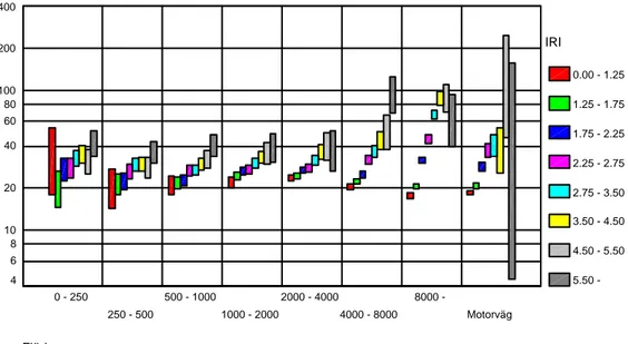
An alternative method to linear regression analysis for studying the relation between accident risk and road surface condition is analysis of variance. As is clear from the above, conditions are good as regards the road surface on most of the road network, and less than satisfactory conditions are rare. The consequence, as stated earlier, is that the linear relations that are estimated mainly apply for the good standard in most parts of the Swedish road network. Using analysis of variance it is possible to detect whether abnormally large rut depths or IRI values have any special effect on accident risk. Analysis of variance does not support the theory that the accident risk on the roads with the deepest ruts, i.e.  18 mm, and which account for barely 2% of the traffic load, should differ dramatically from the accident risk on roads with shallower ruts. The analysis does, though, show that the higher the IRI value the higher the accident risk. The results are presented in figures 2.1 and 2.2.

(17)

Flöde Motorväg 8000 -4000 - 8000 2000 - 4000 1000 - 2000 500 - 1000 250 - 500 0 - 250 400 200 100 80 60 40 20 10 8 6 4 Spårdjup 0.0 - 3.5 3.5 - 5.0 5.0 - 6.5 6.5 - 8.0 8.0 - 11 11 - 15 15 - 18 18

-Figure 2.1 The 95 % confidence interval for expected accident rates in different rut depth and traffic flow classes when IRI is constant within each traffic flow class.

Flöde Motorväg 8000 -4000 - 8000 2000 - 4000 1000 - 2000 500 - 1000 250 - 500 0 - 250 400 200 100 80 60 40 20 10 8 6 4 IRI 0.00 - 1.25 1.25 - 1.75 1.75 - 2.25 2.25 - 2.75 2.75 - 3.50 3.50 - 4.50 4.50 - 5.50 5.50

-Figure 2.2 The 95% confidence interval for expected accident rates in different IRI and traffic flow classes when rut depth is constant within each traffic flow class.

Aquaplaning accidents

Very few accidents occur that are classified as aquaplaning accidents in the police reports compared to the total number of accidents. Of the 80,000 accidents during the years 1992–1998 that were included in the study about 600 were classified as

aquaplaning accidents.

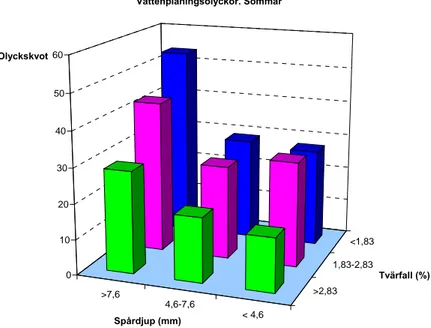
A separate analysis of the aquaplaning accidents was carried out to investigate the influence of rut depth in combination with crossfall. The hypothesis was that the risk for aquaplaning is greatest for large rut depths in combination with a small crossfall, i.e.

(18)

under conditions that give bad water drainage and that means that larger amounts of water may remain on the road surface.

The results from this investigation are shown in figures 2.3 and 2.4 below. It is concluded that the results confirm the hypothesis for when the risk for aquaplaning is greatest. It is also noted that for days with larger amounts of precipitation the influence of crossfall is reduced.

Figure 2.3 The mean aquaplaning accident rate (Olyckskvot) during the summer season in different rut depth (Spårdjup) and crossfall (Tvärfall) classes. All precipitation classes.

Figur 2.4 The mean aquaplaning accident rate (Olyckskvot) during the summer season in different rut depth (Spårdjup) and crossfall (Tvärfall) classes for days with more than 10 mm precipitation. < 4,6 4,6-7,6 >7,6 <1,83 1,83-2,83 >2,83 0 10 20 30 40 50 60 Olyckskvot Spårdjup (mm) Tvärfall (%) Vattenplaningsolyckor. Sommar < 4,6 4,6-7,6 >7,6 <1,83 1,83-2,83 >2,83 0 50 100 150 200 250 Olyckskvot Spårdjup (mm) Tvärfall (%) Vattenplaningsolyckor. Sommar. Mer än 10 mm nederbörd/dygn

(19)

Christensen and Ragnöy (2006) Data and methods

Data from the Norwegian Road Data Bank for the period 1998–2003 was used. Only national roads were included. Road condition data is given lane-wise and an effort was made to place the accidents in lanes as well. The unit in the analysis was 100 m sections in one lane in one year.

For each section there was the following data  County

 Road type (European highway or normal trunk road)

 Accident data (number of accidents). Accidents involving game and accidents at crossings were excluded.

 Rut depth (categorised into five groups: 0–4 mm, 4–9 mm, 9–15 mm, 15–25 mm and > 25mm)

 IRI

 Cross-slope (change in cross slope1₎

 Curve radius

 Average annual daily traffic (AADT)  Percentage long vehicles (heavy vehicles)  Speed limit

 Gradient  Road width.

Two methods of analysis were used, regression analysis and comparison of accidents on the same section in different years.

As the unit of analysis was 100 m sections in one lane in one year there had been no accident on most of the sections, and also there were very few cases where there had been more than one accident on a section. Therefore the dependent variable was whether there had been an accident or not on the section. For this reason logistic regression was used.

1_{The change in cross-slope is defined as the difference between the largest and smallest cross-slope for}

(20)

In a logistic regression the following relation is estimated



        ixi p p _ 1 ln

where p is the probability and x is the explanatory variable. _i

By categorising rut depth in five groups, 0–4 mm, 4-9 mm, 9–15 mm, 15–25 mm and above 25 mm, the effect of rut depth was analysed by four dummy-variables that express the increase in logit relative to the 0–4 mm group.

Since the accident risk on a road depends on many other factors than rut depth, IRI and change in cross-slope a method named “Internal comparison” was also used. To control for the effect of difference between roads the number of accidents is compared to the number of accidents on the same road at a different time in this method.

The internal comparison was carried out in two different ways. One way was to rank the six available years by rut depth and check whether the accidents increase by rut depth. The second way was pair-wise comparison between different rut depth intervals. This meant that only road sections with rut depth in both the compared intervals were included.

Results

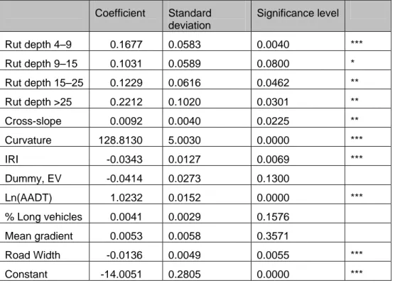
One result from the logistic regressions is shown in table 2 below. To reduce the size of the table some dummy-variables, such as for counties and different speed limits, have been left out.

The logistic regressions showed that the accident risk increases with increasing rut depth. It was however concluded that the relation is not linear. The increase compared to rut depths below 4 mm is greatest for rut depths between 4 and 9 mm and for rut depths above 25 mm.

It was also concluded that there is a negative linear relation between IRI and accident risk, i.e. an increase in IRI entails a reduced accident risk.

For all accidents included, for single-vehicle accidents as well as for accidents during winter, the larger the change in cross-slope the higher the accident risk. This relation does not pertain to head-on accidents or accidents during summer.

The second method of analysis used, i.e. comparison of accidents on the same section in different years, did not result in an equally clear relation between rut depth and accident risk. As this method does not correct for the effect of IRI as in the regression analysis, it is stated in the report that the effect of large ruts may be underestimated since a large IRI will also be common in this case.

(21)

Table 1 Results from the logistic regression. The dependent variable is a dichotomous variable indicating whether there has been an accident or no. The number of units with an accident: 10721.

*: Significant at the 10%-level, **: Significant at the 5%-level, ***: Significant at the 1% level Coefficient Standard deviation Significance level Rut depth 4–9 0.1677 0.0583 0.0040 *** Rut depth 9–15 0.1031 0.0589 0.0800 * Rut depth 15–25 0.1229 0.0616 0.0462 ** Rut depth >25 0.2212 0.1020 0.0301 ** Cross-slope 0.0092 0.0040 0.0225 ** Curvature 128.8130 5.0030 0.0000 *** IRI -0.0343 0.0127 0.0069 *** Dummy, EV -0.0414 0.0273 0.1300 Ln(AADT) 1.0232 0.0152 0.0000 *** % Long vehicles 0.0041 0.0029 0.1576 Mean gradient 0.0053 0.0058 0.3571 Road Width -0.0136 0.0049 0.0055 *** Constant -14.0051 0.2805 0.0000 ***

Source: TØI report 840/2006

Cairney (2008)

A literature review on road surface characteristics and crash occurrence has been carried out by the Austroads. The surface characteristics that have been included in the review are skid resistance, micro and macro texture, rutting and roughness.

Three studies on the effects of rutting are reported (Martin 1999, Favorolo 2000, Ihs 2004 and Cairney 2005). Some results and conclusions reported from these studies are: Favolo:

The main mode of analysis was to plot crash rates per billion km travelled by rut depth category. This analysis showed a progression of crash rate with increasing rut depth, with greatly increasing crash rate when average rut depth exceeded 22 mm. There were however considerable variation in crash rates for higher rut depths. It was furthermore concluded that the percentage of road with this deep ruts (>22 mm) was very small, so even with the much higher crash rate, the number of crashes is still also small.

Another finding was that adverse weather crash rates increased with increasing rut depths at the same rate as all crash rates. It was thus concluded that this is contrary to what would be expected if accumulation of water in ruts is a significant factor in the causation of accidents

Some further conclusions

 Recommendations regarding maximum acceptable rut depth are generally based on either safety or structural and economic considerations.

(22)

 There is no close agreement about what acceptable limits should be Cairney:

The relationship of rutting to crashes was examined on Prince´s Highway West. The distribution of rutting on crash sites was compared to the distribution of rutting on all rural roads. This form of analysis indicates if there is a greater percentage of instances on crash sites or among all sites.

A comparison of rutting distribution at crash sites and all sites was done for ruts < 10 mm, ruts 10–19 mm and ruts 20 mm or deeper.

The findings were

 There is no increase in crash risk associated with rutting until deep ruts (> 20 mm) are reached.

 Although the increase in risk for ruts of 20 mm and deeper may be as high as 60 %, this accounts for less than 3 % of the crashes on the routes studied (only five accidents had occurred at sites with this level of rutting)

 The proportion of wet road crashes was only slightly higher where there was rutting greater than 10 mm, and this was not statistically significant

Othman (2008) Data and method

The objective of this study was to find critical road variables affecting accident rate. The accident data was that reported by the police and the hospitals and was collected from the OLY (accident database with police reported accidents until 2002) and the STRADA (Swedish Traffic Accident Data Acquisition, replaced OLY from 2002) databases, respectively. Only personal injury accidents were included in the study (3,599 accidents, 690 excluded due to missing road condition data).

The road data was collected from the Pavement Management System (PMS) and the national road database (NVDB), which are both owned and maintained by the Swedish Road Administration (SRA). The road variables used in the analysis were speed limit, road type, carriage way width, curvature, grade, super-elevation and road surface variables such as rut depth and road roughness (IRI) (20 m values).

Due to uncertainties in reported accident location the accident localization was

considered to be normally distributed around the real (reported?) accident location. An average value of around 200 m (100 m before and after the 20 m section where the accident was reported to occur) was used for road data. In the sections where no accidents occurred, a mean value of the road parameters was used, where the length of sections varied according to the length of the NVDB sections (0.2–1.5 km).

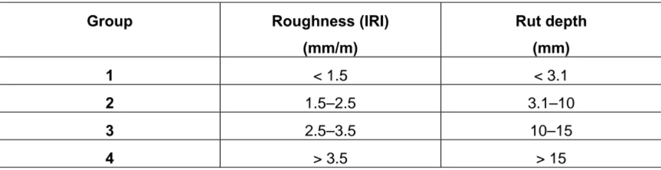
The road surface variables, rut depth and road roughness, were each dived into four groups according to the table below.

(23)

Table 2 Intervals of IRI and rut depth groups.

Group Roughness (IRI)

(mm/m) Rut depth (mm) 1 < 1.5 < 3.1 2 1.5–2.5 3.1–10 3 2.5–3.5 10–15 4 > 3.5 > 15

The investigation was limited to median separated public roads in the western region of Sweden and covered the period 2000–2005.

The accident rate (AR) was used for the analysis and the AR is defined as the number of accidents per Million Vehicle Kilometer (MVKm):

L T AADT accident AR      365 106 accidents per MVKm Where: AR = accident rate

AADT = Annual average daily traffic L = Length of investigated section, km T = Length of investigated time period, year 365 = Number of days per year

The exact method for analysing the data is not very clearly described.

For evaluating the effects of the road variables, it is described that regression analysis techniques were used for modelling the relationship between two or more mentioned variables using a multiple linear equation:

Y = a + b×X1 + c×X2 + d×X3 + ….

Later in the paper it is however said that this method could not be used as originally intended. Regression models were calculated for each individual variable. It was said that each had high correlation coefficients (R2 > 0.88) but that it was not possible to statistically confirm that the relationships were solely related to the selected variable or if other relationships were also present. No evaluation of statistical significance could therefore be presented.

Results

The findings indicated that the highway carriageways with no or limited shoulders have the highest AR when compared to other carriageway widths, while one lane

carriageway sections on 2+1 roads were the safest width. It was also found that large radius right-turn curves were more dangerous than left curves, in particular during lane

(24)

changing manoeuvres. Sharper curves were however found to be more dangerous in both left and right curves. Finally it was found that both rut depth and roughness have a negative impact on traffic safety, i.e. AR increases with both increasing rut depth and increasing roughness.

Chan et al. (2009)

The study has utilized the Tennessee Pavement Management System (PMS) and Accident History Database (AHD) to investigate the relationship between accident frequency in highway segment and pavement condition variables.

A number of negative binomial regression models for various accident types were calibrated with different pavement condition variables including Rut Depth (RD), International Roughness Index (IRI), and Present Serviceability Index (PSI). The modelling results indicate that the RD models did not perform well, except for accidents at night and accidents under rain weather conditions; whereas, IRI and PSI were always significant prediction variables in all types of accident models.

Comparing the three groups of models’ goodness-of-fit results, it was found that the PSI models had a better performance in crash frequency prediction than the RD models and IRI models.

It is suggested that PSI models should be considered as a comprehensive method which can integrate both highway safety and pavement condition measurements into the pavement management system.

TRB (2009)

In 2003 the TRB Surface properties- Vehicle Interaction (ADF90) committee set up a new task group to update the 1983 State of the art report 1 (SOAR1).

Some conclusions from the report are given below for each of the areas that are covered in the report:

1. Tire-pavement friction

It is noted that the influence of surface friction has been the favourite subject of researchers for many years, but also that being able to predict accident risks on the basis of only one condition (skid number) is wishful thinking.

Hazardous situations may for example occur when the friction coefficient varies within or between wheel paths, when friction properties of the surface varies along the direction of travel as well as when marking material with lower skid resistance than the pavement has been applied over larger areas.

2. Roughness, holes and bumps

It is concluded that holes must be relatively large to constitute a significant risk. At common highway speeds a hole must be larger than 60 inches (appr. 150 cm) long and 3 inches (appr. 8 cm) deep.

Consistent roughness is not necessarily a negative influence on safety. Prudent drivers adjust their speed to meet the conditions encountered. Unexpected precipitous change of condition may however constitute an unsafe situation.

(25)

3. Positive effects of road surface discontinuities

Intentional discontinuities such as rumble-strips and bumps normally result in positive effects on safety.

4. Water accumulations.

It is noted that hydroplaning is a low-probability event, primarily because high intensity rainfalls necessary to flood a pavement are low-probability events. Criteria for surface design to further reduce the probability of hydroplaning have been developed.

Splash and spray can affect driver visibility and thus safety. 5. Surface contaminants (ice, snow, mud, sand or gravel)

The primary influence of ice and snow is loss of traction and the magnitude of the loss exceeds most other contaminants.

6. Pavement edges

It is concluded that there is a significant influence of longitudinal pavement edges on vehicle safety. The safety problem is minimized where the pavement drop does not exceed 2 inches (appr. 5 cm) in height or the edge is sloped. 7. Small and large vehicles

The sensitivity/vulnerability to road surface discontinuities is different for small and large vehicles.

Small automobiles: increased probability for injuries during collisions, greater crash involvement rates, road disturbances may pose more severe problems Large commercial vehicles: may be more sensitive to some surface

discontinuities (seen in roughness response and sensitivity to low tire/road surface friction), more severe accidents due to size and mass, unique modes of instability such as jack-knifing and roll-over.

The final conclusions in the report are that

 most drivers are capable of adapting to adverse circumstances, and therefore many potentially dangerous surface problems never cause serious accidents.

 drivers expect satisfactory surface conditions and their expectations have increased over the years

 responsible government entities do not have the available funds to maintain all highways in as-constructed condition. There is therefore a need to prioritize limited funds cost effectively.

2.3 Summary and conclusions

The findings on accident studies related to other road surface conditions than skid resistance are very limited. Actually the only major studies carried out on accident risk and rutting/unevenness during the latest decade appear to be the Swedish and the Norwegian study. Some limited studies have also been carried out in Australia. A common “problem” is that roads with very deep ruts (> 20 mm) are rather rare, and the vehicle mileage as well as the number of accidents is relatively low.

(26)

3 Data collection and construction of databases

3.1 Road condition monitoring

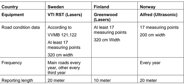
The road condition data used for the analysis is collected with equipment as specified in the table below.

Table 3 Equipment for road condition measurements

Country Sweden Finland Norway

Equipment VTI RST (Lasers) Greenwood

(Lasers) Alfred (Ultrasonic)

Road condition data According to VVMB 121,122 At least 17 measuring points 320 cm width At least 17 measuring points 320 cm Width 17 measuring points 200 cm width

Frequency Main roads every

year, other every third year

Every year

Reporting length 20 meter 10 meter 20 meter

3.2 Collected

data

3.2.1 Overview of data collected from Sweden, Finland and Norway

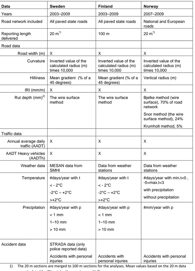
The data collected from the Swedish Transport Administration, the Finnish Transport agency and the Norwegian Road Administration for the analysis is presented in the table below. Data was also initially collected from the Estonian Road administration. Road data was, however, only available for main roads and other roads with AADT>3,000 and accident data only for years 2005–2009. The Estonian road data included IRI and rut depth, but not curvature, hilliness or crossfall. At a later stage of the project it was decided not to carry out any analysis on Estonian data due to the limited amount of data available and considering the results (Chapter 6) obtained for Sweden, Finland and Norway that are based on considerably more data.

(27)

Table 4 Overview of the data collected for the analysis.

Data Sweden Finland Norway

Years 2003–2009 2003–2009 2007–2009

Road network included All paved state roads All paved state roads National and European

roads Reporting length delivered 20 m1) 100 m 20 m1) Road data Road width (m) X X X

Curvature Inverted value of the calculated radius (m) times 10,000

Inverted value of the calculated radius (m) times 10,000

Inverted value of the calculated radius (m) times 10,000 Hilliness Mean gradient (% of a

45 degrees)

Mean gradient (% of a 45 degrees)

Vertical radius (m)

IRI (mm/m) X X X

Rut depth (mm)2) The wire surface

method

The wire surface method

Bjelke method (wire surface), 70% of road network

Snor method (the wire surface method), 24% Krumholt method, 5% Traffic data

Annual average daily traffic (AADT)

X X X

AADT Heavy vehicles (AADTh)

X X X

Weather data MESAN data from SMHI

Data from weather stations

Temperature #days/year with t

< - 2°C -2°C – +2°C >+2°C #days/year with t < - 2°C -2°C – +2°C >+2°C

#days/year with min.t<0 , -5<max.t<3

with precipitation without precipitation

Precipitation #days/year with p

< 1 mm 1–10 mm > 10 mm #days/year with p < 1 mm 1–10 mm > 10 mm #mm/year with p

Accident data STRADA data (only

police reported data) Accidents with personal injuries

Accidents with personal injuries

1) The 20 m sections are merged to 100 m sections for the analyses. Mean values based on the 20 m data are calculated for IRI, rut depth, curvature and hilliness.

2) A comparison of the two main different rut depth calculation principles in Norway, the Bjelke and the wire surface method, is presented in appendix 1.

(28)

3.2.2 Road and traffic data

From here on, a road section is a part (most times 100 m) of a road while a study

section is a part (most times 100 m) of a road a given year.

It was decided that 100 m study sections should be used for the analyses. Therefore we had to merge some 20 m sections from the data deliveries. Moreover in some cases we also estimated non-measured road data values. In this section we describe the merge and estimation process and also some of the data linking process in somewhat detail.

SWEDEN AND FINLAND

The road data was delivered in 20 m sections for Sweden and 100 m study sections for Finland. Therefore we aggregated the Swedish data into 100 m study sections, but required that each of the 20 m sections came from the same homogenous study section. In those cases we let the mean values of the 20 m values represent the 100 m study section. In the cases where we found a fraction of the 100 m distance we adjusted the vehicle mileage (TA) on that study section by multiplication of the same fraction. The same procedure is performed if a road segment is constructed or repaved during the observation year, i.e. we multiply the TA by the fraction of the year it was present. The road condition measurements in Sweden and Finland are only carried out in one direction of the road, except for roads where the two directions are separated as on motorways and 2+1 roads.

Another issue concerns that the road surface measurements do not cover all state roads each year in Sweden and Finland, but all roads in this study have at least one road surface measurement during the period. This means that accidents can be attached to study sections where there are no road condition data, i.e. rut depth and IRI, for that specific year. However, the behaviour of IRI and rut depth is assumed to be rather smoothly changing in time, and linear models can predict the response to a good extent. Therefore, we extended the dataset of the unobserved quantities IRI and rut depth, but also of the quantities ln and by the nearest measurement (for Sweden we also required that the data measurement year didn’t deviate more than one year). The method for calculating rut depth is the so called wire surface method for all roads. The traffic flow, AADT, is presented as the sum for both directions of the road. In Finland this is the case even if the lanes in the two directions are separated as for example on a motorway, whereas this is not the case for the Swedish data material.

NORWAY

The road data was here delivered as 20 m sections, from which we formed 100 m mean values. In some cases where the reporting length was less than 20 m we used weighted mean values to take into account the overlaps. In the cases where we have road

measurements for both directions we averaged over both directions. Here, we did not control the homogeneity of the 100 m distance. For example we could have several speed limits within a 100 m study section, for which we associated only the first found speed limit.

The Norwegian roads are measured by several methods for calculating rut depth, mainly depending on the width of the roads. In the Norwegian material the rut depth on 70 % of the road network is calculated by the Bjelke method, 24 % by the Snor method (the wire

(29)

surface method), 5 % by a third method called the Krumholt method and less than 1 % have unknown method. A comparison between the calculation of rut depth by the wire surface method and the Bjelke method is presented in Appendix 1.

Norwegian traffic flow (AADT) is the sum of the flows in both directions of the road, except for lane separated roads where the flow is for each direction separately.

3.2.3 Accident data

Only accidents involving personal injuries have been delivered and used for the analyses. Each accident is linked to a 100 m study section. This means that no special precautions have been taken to account for the uncertainty that may be present in the given position of the accident. Neither have any accident types been excluded from the delivered data, which means that there are some accidents with game and in crossings included in the material.

SWEDEN

Accident data is gathered from the Swedish Transport Administrations’ accident database STRADA for the years 2003–2009. STRADA includes accidents where there

have been personal injuries and that have been reported to the police. It should be noted however that far from all accidents are reported to the police. Statistics from the medical services show that the number of persons injured in accidents is much higher.

The police authority in the region where the accident has occurred records certain information about the accident directly in STRADA.

The position of the accident is given by coordinates, but there is no information on in which direction of the road or in which lane the accident had occurred. In addition to the coordinates there is also information on the road number and county. For each accident there is information on the type of accident (single-vehicle, head-on, overtaking, rear end, turn off, intersection, cycle/moped, pedestrian, game, other) and the number of fatalities, the number of seriously injured and the number of slightly injured. There is also information on the weather and road surface conditions as reported by the police.

FINLAND

Accidents with injured and killed persons for the years 2003–2009 have been delivered

for the analyses.

The information on each accident collected for the analysis is the position (lane and driving direction was also given) and number of injured and killed persons. There was also information on the type of accident, similar to the information available in the Swedish accident data.

NORWAY

Accidents with injured and killed persons for the years 2007–2009 have been delivered

for the analyses. There was information on the type of accident, but no information on lane or direction in which the accidents had occurred.

(30)

3.2.4 Weather data SWEDEN

Weather data has been received from the Swedish Meteorological and Hydrological Institute (SMHI).

The SMHI has developed a method called MESAN (MESoscale Analysis). In short the analyses are based on a number of different meteorological parameters on such a level that it is possible to describe weather situations with a spatial resolution of about

5–50 km. The analyses are carried out on a grid placed over the area to be analysed. The

MESAN-grid consists of squares that are 22x22 km, which means that Sweden is covered by 960 MESAN squares. MESAN analysis is carried out once every hour. The weather data that has been provided for this project is type and amount of precipitation, air temperature and wind.

The position of the MESAN squares was given in WGS84. A transformation to

SWEREF 94TM, used for positioning the road data, therefore had to be done before this data could be linked to the road network. The weather data from each MESAN square has then been linked to every 20 m section within the square.

For each MESAN square the temperature and precipitation is given for every 30 minutes. This data was aggregated to number of days per year with temperature <-2°C, -2°C – 2°C and > 2°C, as well as number of days with precipitation < 1 mm, 1–10 mm and > 10 mm.

FINLAND

The number of days per year with temperature <-2°C, -2°C – 2°C and > 2°C, as well as number of days with precipitation < 1 mm, 1-10 mm and > 10 mm was delivered for each road segment (length). This data could then be linked to each 100 m study section.

NORWAY

Weather data was delivered for a large number of weather stations (811) covering the whole country. For each station and for each month during the year the number of days with min. temp. <0°C and -5°C < max. temp. < 3°C, with and without precipitation, respectively, is given. The amount of precipitation, rain and snow, each month is given in mm.

Information was also given on which road segments each station should be linked to, i.e. the closest station for each road. From this information it was possible to link each 100 m study section to a station and the corresponding weather data.

(31)

4 Model

approaches

4.1 Introduction

The main objective of this study is to determine how rut depth affects the accident risk of road users.

However, it is assumed that the accident risk also depends on other road condition variables, e.g. longitudinal unevenness, texture, crossfall, geographical position (country), vehicle flow, climate, weather conditions etc.

It should furthermore be pointed out that the accident risk does not only depend on the road condition but also on the road users’ perception and behaviour. One can assume that the road condition constitutes an objective accident risk. The effect of rut depth on the objective accident risk would be how the probability of an accident changes if rut depth changes while a driver tries to travel with the same behaviour, e.g. the same speed, the same distance to the road edge etc. In reality the driver will do some kind of risk assessment, which results in the driver’s perceived accident risk. The perceived accident risk then will affect the driver’s behaviour. The objective and perceived accident risk determine the realised accident risk. The number of accidents actually occurring and registered in the accident data bases is determined by the realised accident risk.

When the objective risk is low the realised accident risk, surprisingly, might be high if the perceived risk is even lower than the objective. Similarly, when the objective risk is high the realised accident risk might be low if the perceived risk is higher than the objective. The relationship between the objective and the realised risk is thus

complicated. As indicated above, the objective of the approaches suggested here is to determine how rut depth affects the realised accident risk.

It is beyond the scope of the study to determine the effect of road condition on the objective and/or the perceived risk. A study has however recently been carried out in the VTI driving simulator where the influence of road surface condition on the drivers perceived risk and driving behaviour was studied (Ihs, 2010). It was found in this study that the perceived risk when ruts were filled with water was significantly higher than when the pavement and the ruts were dry. The drivers clearly compensated for this higher perceived risk by reducing their speed, but also by avoiding driving in the ruts. Accident analysis is in general a very demanding statistical problem and some

alternative approaches have been reviewed in the limited literature survey carried out in this study (see chapter 2.2).

One approach to estimate the effect of rut depth on realised accident risk is by multiple regression analysis, where rut depth is one of several explanatory variables. Such studies have been accomplished in several studies and in later time in the Nordic countries by Ihs et al (2002) and by Christensen and Ragnøy (2006). Another study in the same way would presumably not contribute to the elucidation of the slightly contradictory results from earlier such studies. Instead a procedure is suggested that utilizes the possibilities to determine the effect of rut depth on realised accident risk without confounding from other road condition variables.

(32)

4.2 Summary of different model approaches

A first approach would be to assume a linear relationship between the number of accidents, or rather the logarithm of the expected number of accidents, µ, and the road condition variables with the logarithm of vehicle mileage as offset, i.e.

Model 1 ln ₀ ₁RUT ₂IRI₃RoadWidth....lnTA (1) One problem is that the real relationship might, despite rut, include interactions between the other road condition variables, but there are many, too many, possibilities to include interactions in model 1. Also, the road condition variables might correlate to such extent that the estimated coefficients will be misinterpreted. One way to create fewer and uncorrelated explanatory variables is to replace the other road condition variables by a suitable number of principal components. Each principal component (PC) is a linear combination of the original road condition variables.

Model 2 ln ₀ ₁RUT ₂PC1₃PC2....lnTA (2) However, problem still remains. Implicitly models 1 and 2 assume a monotone

relationship between the road condition variables and the accident risk. Now, the accident risk does not depend only on the road condition in itself but also on how road users perceive it. Then a monotone relationship might not be valid. One way would then be to fit general additive models, i.e.

Model 3 ln ₀  f₁



RUT



 f₂

 

IRI  f₃



RoadWidth



....lnTA (3) The functions in model 3 can be estimated trough splines or moving average regression estimation. However, this approach does not handle the problem with interactions among the other (except rut depth) road condition variables. In that case one would want to estimate an equation such as

Model 4 ln ₀  f₁



RUT



 f₂



IRI,RoadWidth,....



lnTA (4) There is no general method to estimate model 4. One way is to divide the set of road sections into subsets of road sections such that the other road condition variables are comparably homogenous within each subset. Then the outcome of f2 within each subset

should be close to constant. Notice that in model 4 the function f2 can be really

complicated without disturbing the possibility to implement the effect relationship for rut and road accidents. f2 may include interactions, nonlinearities and transformations

but should not have any steps or be very steep. Homogenous subsets might be created through so called cluster analysis.

Another approach to estimate model 4 might be neural networks. The central idea of neural networks is to use nested linear functions to model the target non-linear function. Since the network learns the structure of the nesting of functions as well as the

coefficients of the functions it is extremely flexible and can model almost anything with sufficient amount of data. However, the neural network can be a good classifier in situations where only vague prior assumptions can be made, but may be hard to really understand as the effect of a variable may depend in a complex manner on the states of all other variables. Therefore it is probably not a good candidate approach for the purpose of understanding the influence from rut depth on accident risk or for a maintenance scheme.

(33)

4.3 Chosen

model

approach

The effect of rut depth on accident rates is the main topic for this study. The analysis should be adjusted for other road conditions though their effects on accident rates are not of primary interest. Also, the effects of other road conditions may have a

complicated functional relation, including interactions and more. Under these conditions, an analysis based on model 4 was chosen as main approach.

4.4 Principles of implementation

The objective of the analysis is to determine an effect relationship between the rut depth of the road surface and the accident risk. This should be done in such a flexible way that the relationships may generally be implemented in different kinds of decision support systems. One important application is to study the consequences of changing the maintenance standard, and specifically changing the threshold value for rut depth, on accident risk. In this context the relationship should be described by an equation that gives the relative change in the expected number of accidents for each given change from one rut depth condition to another.

For instance consider a road section with mean rut depth 17 mm. The effect relationship to be determined here will not predict the accident risk on that road section, but rather the relative change in the expected number of accidents if the rut depth would change. Then, if the mean rut depth would increase to 23 mm, the model determined would give a coefficient, h(23|17). So, if the number of accidents during one year with mean rut depth 17 mm were y, then the expected number of accidents another year with mean rut depth 23 mm on the same road section would be h(23|17)×y if vehicle mileage remains unchanged.

The coefficients h(Rut2|Rut1) are expressed in different ways according to the chosen

model approach. Consider the model approaches in section 4.2. Then for equations 1 and 2: h(Rut2|Rut1) = Exp(β1×(Rut2 - Rut1)), and for 3 and 4:

(34)

5 Detailed

description

of chosen model approach

5.1 Introduction

The primary choice of model approach is a somewhat further developed homogenous subsets approach (model 4 in chapter 4.2). A more detailed description is given in chapters 5.2 and 5.3 below.

Due to the complex interaction between the perceived, objective and realised risk, as discussed in chapter 4.1, it is hard to make any assumption on what kind of a functional form the relationship between accident risk and rut depth has. Therefore, in order to avoid making any assumptions rut depth is divided into a number of categories as done by Christensen and Ragnøy (2006). The resulting change-point equation can be

implemented rather easy. Ihs et al (2002) used a similar approach in some analysis. For example if is in RUT depth category . The rut depth categories are different for each country to comply with the categories that are normally used in each country’s guidelines for pavement management.

The proposed model in equation 4 in chapter 4.2 contains the finding of subsets of roads with similar properties. This means, finding homogenous subsets of sections where the function could be approximated constant. For example, , , …

if is the closest subset center. The data partitioning and finding of subset centers is described in more detail in chapter 5.3 below.

As mentioned previously it was decided that 100 m sections should be used for the analysis. It was also decided that separate model variables should be derived for each speed limit and AADT class as defined by each country.

5.2 Model

inference

In the case of a free traffic flow, where cars most often can adapt their speed rather independently to the other drivers the number of accidents would be proportional to the total vehicle mileage on the study section. Even though this is an idealised case the relationship may be approximately true until the point where traffic jams start to occur. Therefore it was decided to exclude from the clustering procedure and instead consider the accident per vehicle mileage in our analysis. Since we consider study sections of almost similar length (100 m) over approximately the same observation time (1 year), most often equals . However, some study sections are less than 100 m, and some roads are constructed or repaved during the observation time, which causes the two to deviate. By these notations we can rewrite equation (4) in chapter 4.2 for a road segment that is in rut depth category and is associated to the homogenous subset as,

ln ln (5)

However, as the number of accidents should be Poisson distributed it implies that the probability for at least one accident may be written as 1 . In practise we rarely observe more than one accident, so therefore for the purpose of inference we reformulate the Poisson regression problem (5) to:

Road user effect models : the influence of rut depth on traffic safety