The determinants of annuitization: evidence from Sweden

Uppsala Center for Fiscal Studies

Department of Economics

Working Paper 2014:13

The determinants of annuitization:

evidence from Sweden

Uppsala Center for Fiscal Studies Working paper 2014:13 Department of Economics September 2014 P.O. Box 513

SE-751 20 Uppsala Sweden

Fax: +46 18 471 14 78

T

:

s

Johannes hagen

Papers in the Working Paper Series are published on internet in PDF formats. Download from http://ucfs.nek.uu.se/

The determinants of annuitization: evidence from

Sweden

Johannes Hagen

November 14, 2014

Abstract

This paper uses unique micro data from a Swedish occupational pension plan

to study the determinants of annuitization. The data is merged with national

administrative data to create a large data set with rich individual background characteristics. The pension can either be withdrawn as a life annuity or during a fixed number of years with a minimum of five years. Low accumulation of assets is strongly associated with the choice of the 5-year payout. Consistent with the predictions of a life-cycle model, retirees who choose the 5-year payout are in worse health and exhibit higher ex-post mortality rates than annuitants. I also find that the parents of annuitants live longer than the parents of those who choose the 5-year payout. This suggests that individuals form expectations about how long they are likely to live based on the life-span patterns of their parents and take this into account when they decide whether to annuitize or not.

Keywords: Annuity puzzle; Longevity insurance; Occupational pension; Adverse selection

JEL classification: D91; H55; J26; J32

∗_{Department of Economics, Uppsala University, Box 513 , SE-751 20 Uppsala, Sweden. email:}

(jo-hannes.hagen@nek.uu.se). I thank James Poterba, Jeffrey Brown, Jonathan Reuter, Svetlana Paschenko, Tarmo Valkonen, Raymond Gradus, Jacob Lundberg, Ponpoje Porapakkarm, Yuwei De Gosson de Varennes, Maria Polyakova, Jean-Marie Lozachmeur, Matthew Zaragoza-Watkins, Monika B¨utler, Mikael Elinder, Per Johansson, Per Engstr¨om, Hannes Malmberg as well as seminar participants at the 2014 IIPF Congress, Uppsala University and the Topics in Public Economics in Uppsala, for their comments. Special thanks to Alecta for providing the data and to P¨ar Ola Grane, Nikolaj Lunin and Lars Callert for helpful discussions. Financial support from the Jan Wallander and Tom Hedelius Foundation is gratefully acknowledged.

1

Introduction

The ongoing shift in pension provision from defined benefit (DB) to defined contribution (DC) has brought more flexibility not only to the accumulation phase of retirement, but also to the decumulation phase. Flexibility during the decumulation phase manifests itself primarily through the introduction of more liquid payout options, such as lump-sums and phased withdrawals, alongside the traditional life annuity.1 Payout phase design involves a trade-off between flexibility and protection from longevity risk. Liquid payout options allow individuals to invest, buy an annuity, leave bequests or increase consumption dur-ing the early years of retirement, but raise concerns that they may trigger individuals to spend the money too rapidly for their own good (Barr and Diamond, 2008). Despite the fact that many countries and private pension plan sponsors have referred to this trade-off to motivate their specific payout phase design, little is known about the characteristics of those who choose to annuitize and those who do not.

The main reason for the limited amount of empirical research on the demand for different payout options is the lack of reliable and comprehensive data. Private pension sponsors and life insurance companies are often reluctant to disclose individual choices, and most public pension systems impose mandatory annuitization. Survey-based data contains rich background information on the retirees, but usually lack actual payout de-cisions. Studies that use data provided by private annuity companies do contain rich information on annuity choices and prices, but are limited with respect to individual background information.

This paper uses unique micro data from a large Swedish occupational pension plan to study the payout decision at retirement. The data is supplied by the second largest occupational pension sponsor in Sweden and includes real payout decisions of about 181 000 individuals. The payout decision involves substantial amounts of retirement savings, as workers are required to contribute a fraction of the wage to whatever occupational pension plan the employer is affiliated to. On average, the occupational pension accounts for as much as 25% of an individual’s total pension income. The company data is merged with national administrative data from Statistics Sweden to get rich individual back-ground information, such as labor market history, education level, health status, and parent longevity. To my knowledge, this is the first paper to combine data from a private life insurance company with administrative data to study the determinants of annuitiza-tion.

Previous empirical studies on the determinants of annuitization have tried to explain the so-called ”annuity market participation puzzle”. The precise nature of the annu-ity puzzle is not well-defined, but traditionally refers to the contradictory nature of low annuitization rates in the private market for annuities in the US and the theoretical predictions of standard standard neoclassical life-cycle model (Benartzi et al., 2011). A seminal paper by Yaari (1965) shows that risk averse individuals without bequest mo-tives will always prefer to hold their assets in actuarial notes (buy an annuity) rather than ordinary notes. A number of explanations have been proposed to explain the low demand for life annuities; the presence of load factors arising from administrative costs, incomplete markets and adverse selection (Mitchell et al., 1999, Finkelstein and Poterba, 2004); bequest motives (Friedman and Warshawsky, 1990, Brown, 2001, Inkmann et al.,

1_{With lump-sums, individuals receive the entire value of the accumulated retirement as a single}

payment, whereas phased withdrawals allow individuals to agree on a schedule of period fixed or variable payments (Antolin, 2008).

2011, Ameriks et al., 2011, Lockwood, 2012); annuity prices (Warner and Pleeter, 2001, Fitzpatrick, 2012, Chalmers and Reuter, 2012), means-tested government benefits (B¨utler et al., 2011, Pashchenko, 2013), and pre-annuitized first-pillar pension income (Bernheim, 1992, Dushi et al., 2004, Beshears et al., 2011). More behaviorally oriented phenomena, such as loss aversion, default provision and framing have also been put forward as poten-tial explanations for the annuity puzzle (Brown, 2007, Brown et al., 2008, Agnew et al., 2008, Benartzi et al., 2011, Beshears et al., 2014).

The payout decision I study in this paper concerns whether individuals withdraw their occupational pension as a life annuity or during a fixed number of years.2 Under the life annuity, the individual’s pension capital is converted into a monthly payment stream that is paid out as long as the individual is alive. In contrast, there is no mortality link, and hence no annuity component, in the fixed-term payout options. At retirement, the indi-vidual specifies the time period during which the pension capital should be withdrawn. Payments cease after the preferred time period has expired. Payments also cease if the individual dies before the specified payout period has elapsed.3 The fastest rate at which the pension capital can be withdrawn is over five years.

The average annuitization rate over the whole period is 76%. This number is compara-ble to the annuitization rates in papers that study similar pension settings (Chalmers and Reuter, 2012, B¨utler and Teppa, 2007). Thus, studies on payout decisions in mandatory second-pillar pension plans, including this one, raise less concerns about the existence of an annuity puzzle than what the size of private annuity markets does.4 _{The fraction of}

retirees choosing fixed-term payout options rose from 20% in 2008 to 31% in 2013. The 5-year payout is by far the most popular fixed-term payout option, chosen by more than 70% of the individuals that did not choose the life annuity.

I carefully analyze some of the determinants of annuitization that have been discussed in the literature. I pay particular attention to the role of health and life expectancy (ad-verse selection), retirement wealth and the tax consequences of choosing different payout options. As for adverse selection, I analyze whether there are systematic relationships between the length of the payout on the one hand, and ex-post mortality on the other. I also investigate whether individuals in bad health self-select into fixed-term payouts. Health is proxied by the number of days an individual has been absent from work due to illness during a pre-specified age interval prior to retirement. Finally, I use information on parent mortality to create proxies for an individual’s life expectancy.

The results show that individuals in bad health are more likely to choose the 5-year payout. Ex-post mortality rates also signal the presence of adverse selection. Individuals who choose the 5-year payout are 73% more likely to die within four years after claiming than annuitants. I also find that the parents of annuitants live longer than the parents of those who choose the 5-year payout. This suggests that individuals form expectations about how long they are likely to live based on the life-span patterns of their parents and take this into account when they decide whether to annuitize or not.

Small stocks of pension capital are more likely to be withdrawn during a fixed number

2_{In international voluntary and involuntary annuity markets that offer different payout rates,}

indi-viduals normally get to choose between a life annuity and a lump-sum.

3_{In defined contribution schemes, an individual can buy survivor insurance, which means that the}

remaining pension capital will be paid out to his or her partner or children. The combination between a fixed-term payout and survivor insurance is sometimes referred to as a fixed-term annuity.

4_{Annuitization rates in U.S. DB pension plans that offer a lump-sum are typically lower than this,}

ranging from 25% to 50% (Mottola and Utkus, 2007, Benartzi et al., 2011, Previtero, 2012, Banerjee, 2013).

of years. Although small capital stocks often signal low pre-retirement income, this effect seems to be mainly driven by high rates of time preference rather than by the income level of the individual. Payout preferences are fairly constant across the income distribution, except among individuals at the very top. High-income individuals, particularly those with large capital stocks, are much less likely to choose the 5-year payout. Tax-adjusted calculations of the money’s worth ratio (MWR) of the life annuity suggest that high-income individuals might choose long-term payouts to avoid a higher effective marginal tax rate. In fact, the expected present discounted value (EPDV) of the 5-year payout falls by as much as 26% for the richest 10% when taxes are accounted for.

The rest of the paper is organized as follows. Section 2 provides a brief description of the Swedish pension system, with emphasis on the structure of the occupational pension plan for white-collar workers. The potential determinants of the demand for different payout options are discussed in section 3. Section 4 describes the data and section 5 reports the results from several empirical specifications. Section 6 concludes.

2

Background Information

In this section, I describe the main components of the Swedish pension system. I pay par-ticular attention to the structure of the occupational pension system, in which individuals face different payout options.5

2.1

The structure of the Swedish pension system

Sweden’s pension system has two main pillars, a universal public pension system and an occupational pension system for workers whose employer is tied to some occupational pen-sion plan. The public penpen-sion is the most important source of penpen-sion income, amounting to 50-80% of an individual’s total pension income. Mandatory annuitization applies to all pension wealth in the public pension system. The public pension system has in itself three tiers, of which two are earnings-related and DC. They insure income up to a certain threshold level called the ”income ceiling”.6 _{The third tier is a means-tested pension}

supplement that ensures individuals with no or low pension income from the earnings-related component a minimum standard of living in retirement.

The second pillar consists of a number of different occupational, employer-provided pension plans. Occupational pension plans are constructed and thought of as supple-ments to the public pension system, as they provide pension benefits above the income ceiling in the public pension system. The occupational pension therefore plays a more important role for total retirement income for individuals with earnings above the ceiling than for those below. Contributions to the second pillar are essentially proportional to in-sured income up to the income ceiling. The employer is mandated to contribute between 4-6% of the wage portion of the insured that does not exceed the income ceiling. For wage portions above this threshold, contribution rates are much higher, typically around 30%. There is also a third pillar for voluntary savings available to anyone who cares to supplement the retirement income provided by the first two pillars. Third-pillar savings are tax-deferrable and the pension capital can be withdrawn during a fixed number of

5_{A detailed description of the Swedish pension system can be found in Hagen (2013).}

6_{The ceiling is currently at 7.5 income base amounts (IBA). For 2013, this means that no pension}

years with a minimum of five years.7

2.2

Occupational pension for white-collar workers

Most occupational pension plans are designed and implemented at the union-level. In fact, the four largest occupational pension plans cover around 90% of the total work force. Two of these plans cover workers employed in the public sector. The other two pension plans cover white-collar workers and blue-collar workers in the private sector, respectively. For data availability reasons, this study focuses on payout patterns for white-collar work-ers in the private sector.

In the last two decades, all major occupational pension plans have undergone sig-nificant changes. Most importantly, all plans have been changed from DB to DC or a mixture of the two. In the old DB-dominated regime, individuals had relatively little control over their occupational pension assets. Transferability of accumulated assets was limited and benefits after retirement were typically received in the form of life annuities. The transition to DC has had important implications for the control individuals have over their assets. In particular, all pension plans have introduced fixed-term payouts as an alternative to lifelong annuities. Since the transition to DC is still ongoing, the majority of today’s retirees still have some part of their occupational pension wealth in old DB plans where annuitization is mandatory. White-collar workers, however, face no restriction on the fraction of wealth that can be withdrawn during a fixed number of years. More on this below.

The pension plan for white-collar workers is called ITP. The transition of the ITP plan to DC began as late as in 2006, which implies that all cohorts in my sample belong to the old pension plan.8 _{The most important source of occupational pension income}

for white-collar workers in this pension plan is DB. This component is referred to as ITP2.9 _{Before 2008, pensions from ITP2 were always paid out as life annuities. However,}

starting in 2008, ITP2 introduced fixed-term payouts as an option to annuitization. In fact, ITP2 is the only DB plan in Sweden that allows for fixed-term payouts. Because the payout decision accrues to all ITP2 pension wealth, substantial amounts are at stake in the payout decision among this group of workers.

There is also a DC component within the ITP plan, called ITPK.10 Since ITPK

pen-7_{In 2002, 42% of individuals aged 18-64 years saved in tax-deferred pension accounts (Johannisson,}

2008). Tax-deferred pension accounts are particularly beneficial for high-income earners because of the progressive tax schedule.

8_{In fact, the first cohort to be affected by the new DC pension plan, called ITP1, are those born in}

1979.

9_{Benefits from ITP2 are calculated based on the pensionable wage w, which, in effect, is the final}

wage. Pensionable wage also incorporates benefits in kind, compensation for regular shift work, time on call and stand-by time at the time of retirement. The replacement rate is higher for pre-retirement income that exceeds the income ceiling in the public pension system. The ITP2 benefit is calculated according to equation 1, where wi denotes the wage portion related to IBA i:

IT P = 0.1w<7.5 IBA+ 0, 65w7.5−20 IBA+ 0.325w20−30 IBA (1)

For full ITP2, 30 whole entitlement years are required. An entitlement year can be earned from age 28 and is earned if the individual worked at least 20% of full-time. Earned ITP2 entitlement years are transferred to the new employer if the individual changed job.

10_{ITPK is less important than ITP2 for the individual and normally amounts to 10% of the final wage}

if it is paid out over five years. Each month, the employer sets aside 2% of the wage to ITPK from the time that the employee has attained the age of 28. The size of the ITPK benefit is determined by the

sion wealth cannot be withdrawn as a life annuity, but during a fixed number of years only, the analysis on payout choices in the ITP plan will focus primarily on the DB com-ponent.

Employer-sponsored contributions to the second pillar are managed by some occupa-tional pension company. Each pension plan has its own ”default” managing company, meaning that if the individual takes no action, her pension assets will be managed by that pension plan’s default company. The ITP plan allows individuals to transfer DC assets between pension companies in contrast to DB pension wealth, which is tied to the default company. Since this paper focuses on payout patterns in the DB component, self-selection out of the default company is not a concern.

The normal retirement age for white-collar workers is 65. A few months before plan participants reach this age, they receive information about the different payout options from the managing pension company. The information letter clearly states the size of the monthly benefit under each payout option. If the participant takes no action, the occupational pension is paid out as a life annuity from age 65. However, opting out is easy and requires no time-consuming paperwork. The individual simply ticks the box that corresponds to the preferred payout option in the information letter.

The life annuity guarantees the retiree a stream of money right up until the point of death, whereas payments cease after a certain date under the fixed-term payout options. There are different conversion factors for each payout option, i.e. the factor at which the accumulated pension capital is converted into a monthly payment. The conversion factors depend on the individual’s age (life expectancy) and assumptions about the rate of return on the pension capital, but is independent of gender and marital status. The occupational pension plan I study in this paper offer five payout options: a life annuity, or fixed-term payouts over 5, 10, 15 or 20 years.

2.3

Tax treatment of occupational pension income

Retirement income from public and private pension plans are subject to the same tax rules as income from labor.11 _{A proportional local tax rate applies to all earned income}

and taxable transfers which includes pension income. The mean local income tax in 2013 was 31.73% with a minimum rate of 28.89 and a maximum rate of 34.52. For pension incomes above a certain threshold (SEK 450 300 in 2013) the taxpayer also has to pay a central government income tax. The central government income tax schedule consists of two brackets; the marginal tax rates in each bracket are 20% (for incomes between 450 200 and 620 600 in 2013) and 25% (for incomes above 620 600), respectively. Before computing the individual’s tax liability, a basic deduction is made against the individual’s total income. The basic deduction is phased in at lower income levels and phased out at higher income levels with consequences for the marginal tax rate in these income intervals.12

Figure 1 shows the marginal and average tax rate as functions of pension income for individuals who have turned 65 and have no labor income. It is clear from the figure that the progressivity of the tax schedule will have implications for individuals’ valuation

accumulated wealth in the individual’s retirement account.

11_{See Edmark et al. (2012) for a detailed description of the Swedish income tax system.}

12_{The basic deduction for individuals aged 65 and above is higher than for those below this age. This}

implies that the thresholds in the central government tax schedule are somewhat lower for individuals below age 65. In 2013, the basic deduction for individuals aged 65 and above was phased in between SEK 45 000 and SEK 166 900 and phased out between SEK 212 300 and 538 700.

Figure 1: Marginal and average tax rate in 2013 0 .2 .4 .6 0 200000 400000 600000 800000

Annual retirement income (SEK)

Marginal tax rate Average tax rate

of different payout alternatives in the occupational pension, especially for high-income earners with incomes above the central government tax threshold.13

3

Empirical Predictions

This section summarizes the potential determinants of annuitization that have been dis-cussed in the literature and that can be tested empirically with the data at hand.

The choice between the life annuity and any of fixed-term payout options should depend on the expected present discounted value (EPDV) of each payout option. The EPDV of a particular payout depends in turn on the price of that payout option, and on the characteristics of the individual. Asymmetric information about retiree life ex-pectancy is the most natural source of variation in the EPDV of a given payout option across individuals.

In a standard life-cycle model, life annuities provide higher rates of return than other risk-free investments, because they transfer assets from those who die to those who sur-vive. The additional rate of return on life annuities is referred to as the ”mortality premium”.14 _{However, because fixed-term payouts also transfer assets from those who}

13_{High marginal tax rates are also avoidable during the accumulation phase of retirement savings.}

Employees can give up the right to part of the cash remuneration due under his or her contract of employment in return for the employer’s agreement to provide the employee with additional pension contributions (salary sacrifice or ”l¨onev¨axling”). A special tax applies to these contributions, which is lower than the regular payroll tax. The pension contribution will therefore be larger than the foregone wage, a system which. Salary sacrifice is particularly beneficial for taxpayers with high levels of income. Employers also gain from this since pension contributions to occupational pension plans are deductible.

14_{Yaari (1965) derives conditions under which risk averse individuals with an unknown date of death}

and without bequest motives always prefer to hold their assets in actuarial notes (buy an annuity) rather than ordinary notes. Davidoff et al. (2005) extends the analysis and show that individuals benefit from converting a significant fraction of their assets into life annuities even in the presence of incomplete markets for life annuities. Feigenbaum et al. (2013), on the other hand, show that the welfare effect of

die to those who survive it is not clear that the life annuity should provide a higher rate of return. In fact, the EPDV of the ITP life annuity is somewhat lower than the EPDV of the fixed-term payouts, which implies that fixed-term payouts would be the most rational choice for the average plan participant. If there is an option value asso-ciated with holding liquid assets, fixed-term payouts should become even more attractive.

3.1

Health, mortality and life expectancy

An individual’s health condition and life expectancy should influence the annuitization decision because annuities hedge longevity risk. A lifelong annuity should be less valuable to someone in poor health who expects to live shorter than the average participant in the pension plan. For our setting, this implies that individuals who expect to live long should prefer life-long annuities to fixed-term payouts with short payment horizons and vice versa.

The most compelling evidence of the presence of adverse selection in life annuity mar-kets is when ex-post mortality rates are lower among those who buy life annuities than among those who do not. Finkelstein and Poterba (2004) report evidence of adverse selec-tion of long-lived individuals into private annuity markets in the UK. Because fixed-term payouts were introduced in 2008, I can track mortality only within a few years after the claim was made. If there is adverse selection, ex-post mortality rates should be higher among individuals who choose fixed-term payouts.

I get information about an individual’s health status from social insurance register data. The most straightforward health measure is based on the number of days an in-dividual has been absent from work due to sickness. The medical literature has shown that sickness absence can be used as an integrated measure of physical, psychological, and social functioning in studies of working populations (Marmot et al., 1995, Kivim¨aki et al., 2003).

However, health is a non-perfect measure of subjective life expectancy. Two individ-uals with similar health status can have very different beliefs about how long they will live relative to the cohort average. Such differences in beliefs might reflect family-specific rather than individual-specific characteristics. A very intuitive and simple way for an individual to get information about how long she is likely to live is to look at life-span patterns among family members. It has been shown that individuals take (same-sex) parent longevity into account when assessing their own life horizons (Van Solinge and Henkens, 2009). I use information about the age at death of individual i ’s parents to proxy individual i ’s life expectancy.

3.2

Retirement wealth

Wealth has been shown to be an important determinant of the payout decision.15 _Ideally,

wealth should be measured before annuitization takes place and include both pension and non-pension financial wealth. However, because the data does not contain information on non-pension financial wealth, the analysis is restricted to (occupational) pension wealth.

annuitization is ambiguous in general equilibrium on account of pecuniary externalities.

15_{Some studies that find that (retirement) wealth and pre-annuitized income are important}

determi-nants of the payout decision are Inkmann et al. (2011), Chalmers and Reuter (2012), B¨utler and Teppa (2007) and Pashchenko (2013).

Pension income from other occupational pension plans and the public pension system should be thought of as pre-annuitized wealth.16 _{These may act as substitutes for a life}

annuity in the ITP plan. Because the marginal value of insurance declines with the level of insurance, the value that a retiree attaches to the incremental life annuity should fall with the level of pre-annuitized income.

I predict that retirees who are more reliant on ITP benefits because they spent most of their career working for ITP employers should be more likely to choose the life annuity. The marginal effect of income from other occupational pension plans on the probability of choosing the life annuity should therefore be negative. In the same way, ITP pension wealth should be negatively correlated with the length of the payout. In other words, the value of the ITP benefit under the life annuity should have a negative effect on the probability of choosing the life annuity.

However, the relationship between retirement wealth and payout preferences is po-tentially more complex than this. Firstly, it has been shown that small outcomes are discounted at higher rates than greater ones are (Frederick et al., 2002). Individuals with low levels of occupational pension wealth might find life annuities unattractive since their wealth would be translated into a very small payment stream. Low levels of retirement wealth would then be associated with a higher propensity to cash out the money at the fastest possible rate, i.e. over five years. At the same time, low levels of capital might be the result of high discount rates due to low investment in education.

Secondly, if individuals prefer to cash out small amounts of retirement wealth and if the researcher has an incomplete picture of individuals’ annuitization decisions in different pension plans, low annuitization rates might reflect the distribution of account balances rather than the distribution of preferences (Benartzi et al., 2011).

Another reason why we would expect individuals to withdraw their pension during a fixed number of years is to become eligible for different kinds of means-tested benefits and reduced fees for elderly care after the pension payments have ceased.17 _{This ”moral}

hazard” issue is, however, difficult to investigate empirically. Not enough time has passed since the introduction of fixed-term payouts to see if individuals who choose the 5-year payout are more likely to receive means-tested benefits five years after claiming.

3.3

Annuity pricing and tax treatment

Variation in the value of life annuities arise not only from differences in retiree characteris-tics, but also from differences in annuity pricing. An individual should prefer the annuity if the price of the annuity (the initial premium or the foregone lump sum) is lower than the expected benefit from smoother lifetime consumption. Chalmers and Reuter (2012) show that retirees respond very little or nothing at all to changes in the price of the life annuity option. They argue that low price elasticities of demand are due to the complex-ity of evaluating the EPDV of different payout options. However, based on the relatively high demand for the better than actuarially fair-priced life annuity that they observe in their setting, they suggest that retirees may still respond strongly to large, salient changes in annuity prices.

16_{Pension wealth in occupational pension plans other than the ITP plan can be viewed as pre-annuitized}

wealth since these plans only allow limited amounts of DC capital to be withdrawn as fixed-term payouts for the cohorts studied in this paper.

17_{There are two important income-tested benefits in the Swedish pension system: a housing supplement}

Large changes in the value of life annuities can arise from the tax treatment of retire-ment income. The progressivity of the tax schedule implies that the effective marginal tax rates under the fixed-term payouts are higher than under the life annuity. In this section, I extend the traditional measure of an annuity’s value, the ”money’s worth ratio” (MWR), to account for the tax treatment of pension income.18

The MWR of a life annuity is the ratio of the expected present discounted value (EPDV) of the flow of payments made by an annuity to the money paid for an annuity, where the money paid for an annuity typically refers to the foregone lump sum payment. In my setting, the value of the money paid cannot be determined since there is no lump sum option, nor information in the data on the exact amount of contributions paid to the ITP plan. This implies that the EPDV of the life annuity must be related to the EPDV of each fixed-term payout option in order to find the MWR of the life annuity. The EPDV of payout option p purchased by an individual of age a is given by:

EP DV_ap(B) = Bp

T

X

i=1

πt,t+i(1 + rt)−i (2)

where πt,t+i is the probability of someone living i more years, believed in year t, Bp is

the gross benefit received by an individual per year under payout option p, rt is the

appropriate discount rate for payments received in period t, expressed at an annual rate, and T is the last period of payment.19 _{For life annuities, T is chosen so that π}

t,T ≈ 0,

which happens when T = 45 (i.e. no one lives beyond age 110 years, assuming a = 65. For the 5-year payout option, T = 5, for the 10-year payout option T = 10 and so on.

The MWR of the life annuity is then the ratio of the EPDV of the life annuity to the EPDV of any of the fixed-term payout options. For example, the MWR of the life annuity with respect to the 5-year payout option is expressed as:

M W RAnnuity/5−year = EP DV

Annuity a

EP DVa5−year

(3)

If this expression is equal to one, the life annuity and the 5-year payout have equal expected present discounted values.

The net-of-tax MWR is defined as the ratio between the EPDV of the net benefit under the life annuity and the EPDV of the net benefit under any of the fixed-term payout options. I replace the gross benefit Bp _{in equation 2 with the net benefit B}p,net_.

The EPDV of a net benefit is given by

BP,net = Bp− [T (Bp_{, I, a) − T (0, I, a)] (4)}

where T (Bp, I, a) is total taxes paid under payout option p, T (0, I, a) is total taxes paid when the individual has no occupational income, I is other pension income and a is age.

18_{MWRs of annuities have been used in a number of earlier studies, including Friedman and}

War-shawsky (1988), Brown and Poterba (2000), Mitchell et al. (1999), Finkelstein and Poterba (2004) and Chalmers and Reuter (2012).

19_{When estimating the expected present discounted value of each payout option, I use the mean yield}

on ten-year Treasury notes in year t − 1, and I use the mortality tables published by Statistics Sweden for year t.

The average tax rate can then be written as

τ = T (B

p_{, I, a) − T (0, I, a)}

Bp (5)

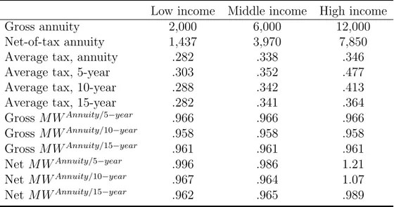
Table 1 reports average tax rates and MWRs for three representative individuals. The first row reports the gross benefit, Bp, under the life annuity. The second row reports the corresponding net benefit. Due to the progressivity of the tax schedule, the average tax rate decreases with the length of the payout for a given level of income. Short payout horizons result in higher monthly income and higher marginal taxes. Note that the aver-age tax rate for low- and middle-income individuals is only two percentaver-age points higher under the 5-year option than under the life annuity compared to almost 14 percentage points for the high-income individual. For the high-income individual, this corresponds to an increase in the average tax rate of 34%. The reason for this is that the high-income individual reaches the central government tax threshold under the 5-year payout option. The table also reveals that the gross MWR of the life annuity with respect to each fixed-term payout is somewhat below one.20 The picture changes when taxes are taken into account. The net-of-tax MWR calculations show that the fixed-term payouts be-come less attractive relative to the life annuity. This is particularly true for the 5-year payout. For example, the MWR of the life annuity with respect to the 5-year payout for the middle-income individual increases from 0.966 to 0.986 when taxes are accounted for. The corresponding net MWR for the high-income individual amounts to as much as 1.21. These changes reflect the changes in average tax rates across individuals with different income and across payout options.

Based on these results, I predict that the demand for fixed-term payouts with short payment horizons (5 and 10 years) will be lower among individuals in the top part of the income distribution (and the pension capital distribution). The tax effect on the money’s worth of annuities for low- and middle-income individuals are probably too small to generate important variation in demand.

3.4

Bequest motives, socio-economic background and

demo-graphic characteristics

Differences in retiree characteristics that relate to socio-economic background and demo-graphics can also generate cross-sectional differences in the expected utility associated with life annuity payments.

Bequest motives have been put forward as one of the most important explanations for the annuity puzzle. In the absence of bequest motives, any wealth that an individual is holding at death does not contribute to utility, so there is no reason to forego the higher rate of return on annuities that arises from the mortality premium (Brown, 2001). With bequest motives, however, that is when a parent household cares not only about its own lifetime consumption but also about the consumption of its descendants, the individual will not always benefit from annuitizing his entire wealth at retirement. The individual now gets utility from the financial wealth which he holds at death and that is bequeathed to his heirs. As a result, full annuitization may not be optimal. Given that the EPDV of fixed-term payouts is somewhat higher than that of the life annuity for the majority of

20_{This holds for discount rates less than or equal to 1.1%. The mean yield on ten-year Treasury notes}

Table 1: Tax-adjusted money’s worth ratios (MWR) of life annuities

Low income Middle income High income Gross annuity 2,000 6,000 12,000 Net-of-tax annuity 1,437 3,970 7,850 Average tax, annuity .282 .338 .346 Average tax, 5-year .303 .352 .477 Average tax, 10-year .288 .342 .413 Average tax, 15-year .282 .341 .364 Gross M WAnnuity/5−year _{.966 .966 .966} Gross M WAnnuity/10−year _{.958 .958 .958} Gross M WAnnuity/15−year _{.961 .961 .961} Net M WAnnuity/5−year _{.996 .986 1.21} Net M WAnnuity/10−year _{.967 .964 1.07} Net M WAnnuity/15−year _{.962 .965 .989}

Note: This table reports tax-adjusted calculations of the money’s worth (MW) of the life annuity for three representative individuals. Each individual retires at age 65 and has no labor income. The public pension for the low-, middle- and high-income individual amounts to SEK 10 000, 15 000 and 20 000, respectively. The first row reports the ITP benefit paid out as an annuity. The second row reports the net-of-tax ITP benefit. The relative importance of the ITP benefit increases with the income level. The benefit formulas and the tax schedule of year 2013 are used.

ITP retirees, fixed-term payouts should be the preferred alternative for individuals with bequest motives.

Empirical findings on the effects of bequest motives on payout decisions are mixed. To test for the effect of bequest motives, researchers typically proxy intentional bequest motives with the presence of children. Brown (2001) and Inkmann et al. (2011) find insignificant effects of the number of children on the payout decision. B¨utler and Teppa (2007) lack data on the presence of children, but find that divorced/widowed men cash out more than single men, which is indicative for the presence of a bequest motive. I follow the literature and proxy bequest motives with the presence of children.

Since men live shorter than women on average, I predict that fixed-term payments are more valuable to male retirees, who should expect to receive fewer payments than female retirees. The results in the literature with respect to gender are also mixed. Inkmann et al. (2011) and B¨utler and Teppa (2007) report higher cash-out rates for women, proba-bly reflecting availability of alternative sources of income, whereas Chalmers and Reuter (2012) find the opposite.

Labor market participation at the time of withdrawal might impact the decision to annuitize. The tax consequences of positive labor income after retirement, particularly in combination with large pension capital stocks, might drive down the demand for fixed-term payouts.

4

The Data

4.1

The datasets

I use data from a pension company called Alecta. Alecta manages occupational pensions for approximately two million private customers, making it the second largest occupa-tional pension company in Sweden and one of the largest owners on the Stockholm Stock Exchange. Alecta is the default option in the ITP plan, which means that they admin-istrate pension contributions and pension payouts for private-sector white-collar workers whose employer is part of the ITP plan.

The data consists of information on all Alecta’s customers that retired over a six-year period ending in 2013. The sample includes 181 180 individuals born between 1943 and 1951. Most importantly, it contains information on in which year and month each retiree claimed the occupational pension and under which payout option it is withdrawn.

The company data is merged with register data from Statistics Sweden to obtain rich individual background information. The data also contains birth and mortality informa-tion for the biological parents of these individuals. The data is derived from the Longi-tudinal Integration Database for Health Insurance and Labour Market Studies (LISA). LISA covers the period 1990-2011, which implies that I can create panels of past income streams for each individual in the sample. From the panel structure of the register data, I construct one observation per retiree with variables that are likely to be determinants of the payout decision.

Since the register data ends in 2011, there is no contemporaneous income information for individuals that retire in 2012 and 2013. In order to get a full picture of the post-retirement financial situation for these individuals, I restrict the sample to payout choices made in or before year 2010 when the analysis includes current income streams, such as labor market earnings and pension income from other occupational pension plans.

4.2

Descriptive statistics

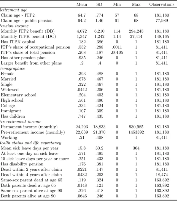
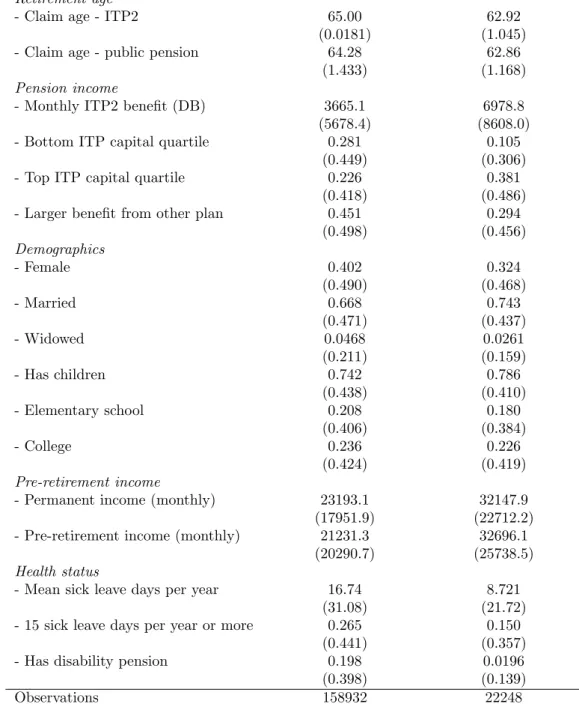
Table 2 reports summary statistics for all key variables. All numerical variables are ex-pressed in constant 2013 Swedish Crowns (SEK).

The average monthly benefit from the DB component, ITP2, amounts to SEK 4080. The large variation in the size of the benefit across individuals (standard deviation of SEK 6216) is a direct result of large differences in pre-retirement income and the con-struction of the ITP plan, which replaces more income above the income ceiling. 82% in the sample receive ITP benefits from the supplementary DC component called ITPK. The average ITPK benefit among these individuals amounts to SEK 1347.

Pre-retirement income is defined as the average income from labor during the five years preceding retirement. The average pre-retirement income is SEK 22 639. The in-dividual’s permanent income is defined as the average monthly income between age 51 up to retirement. Permanent income should reflect lifetime earnings better than pre-retirement income, and is also more strongly correlated with pre-retirement wealth. Active participation in the labor market after retirement (”Working” in table 2) is defined as having labor earnings greater than two income base amounts in the year succeeding the claiming year.21 _{In fact, more than 20% are classified as working based on this definition.}

21_{This corresponds to a monthly income of SEK 7 400 or 30% of the average permanent income. This}

We also see from the table that some white-collar workers receive retirement benefits from other occupational pension plans. On average, retirement benefits from the ITP plan make up 55.2% of the total occupational pension income. 93% receive income from some other occupational pension plan. For 20% of the sample, this income is bigger than what they get from the ITP plan. Public pension benefits are on average 33% larger than total occupational pension income.22

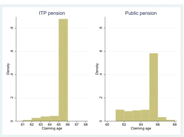
The average age at which retirement benefits from ITP are claimed is 64.7. ITP ben-efits can be withdrawn from age 55 with an early retirement penalty of 7% per year. The left-hand panel of figure 2 illustrates the claiming behavior of the white-collar workers in the sample. The graph shows that almost 90% claim the occupational pension when they turn 65. A number of factors contribute to this pattern: pension rights are not earned after the age of 65, benefits are automatically paid out at this age, 65 is usually referred to as the ”normal retirement age” and the social norm that retirement should happen at this age.

This distribution of retirements might not, however, reflect the true retirement be-havior of the the retirees in the sample. Some individuals that retire at age 65 might live off retirement income from other sources, such as the public pension system or other occupational pension plans. The right-hand panel of figure 2 plots the distribution of claims of the public pension. Indeed, the spike at age 65 is less pronounced (around 60% start to draw their public pension at this age), more people claim at earlier ages.23

Although very few people claim their pension after the age of 65 (as seen in figure 2), they may still be active in the labor market past this age. Figure 3 plots the evolu-tion of labor income in a two-year window around the year in which the ITP benefit is claimed. The sample is split into four groups based on permanent income. Labor income falls considerably in all income groups prior to retirement and continues to do so after retirement. Income levels before retirement are already low for retirees in the two lower income groups, supporting the notion that some individuals live off other types of re-tirement income before claiming the occupational pension. The figure also suggests that post-retirement labor market participation is an important phenomenon among high-income earners. Choosing the life annuity or any of the long-term fixed-term payouts in order to avoid a higher marginal tax rate becomes even more relevant for individuals with large pension payments who also work.

39.3% of the sample are women. An individual’s marital status is based on what is observed at the time of retirement. 67.8% and 32.2% of the sample are married24 and singles, respectively, and 4.4% are widowed. A high school degree is the highest educa-tion level for the majority (56.1%). 23.4% has a college degree and 20.4% finished only elementary school.

Information on health and mortality is also collected from LISA. I use individual-specific information on sickness absence as a proxy for health.25 _{I look at sickness absence}

22_{The importance of the occupational pension in relation to the public pension is likely overestimated}

in this case because we simply look at monthly income streams without taking into account the payout horizon of the occupational pension benefits.

23_{Note that it is possible to claim public pension even after the age of 68, but this is the maximum at}

age to which the oldest birth cohort (1943) can be tracked.

24_{Includes co-habiting partners.}

25_{An employee that calls in sick receives sick pay from the employer the first 14 days of absence. After}

14 days, the employer reports the case to the Swedish Social Insurance Agency (F¨ors¨akringskassan), who pays out a sickness benefit that amounts to about 80% of the individual’s salary. The data in this study contains information on the number of days individuals receive sickness benefits from F¨ors¨akringskassan.

Figure 2: Histogram of claiming ages, ITP and public pension 0 .2 .4 .6 .8 Density 61 62 63 64 65 66 67 68 Claiming age ITP pension 0 .2 .4 .6 .8 Density 60 62 64 66 68 Claiming age Public pension

incidence between age 51 up to retirement. The mean number of days per year of sickness absence in the sample is 15.8 (standard deviation 30.2 days). About 43% of the sample never received sickness benefits during this period.

Mortality data is available up to year 2012. For this reason, the sample is restricted to claims made before 2011 and 2009 when I look at mortality within two and four years after the claim date, respectively. 2.2% of the sample die within two years after claiming and 4.3% within four years. These mortality rates are sufficiently high to allow meaning-ful study of retiree mortality and adverse selection.

Information on parents’ date of birth and mortality is available for 90% of the sample. The remaining 10% have parents who never lived in Sweden and do not show up in the registers for this reason. These individuals are excluded from the sample in the analysis of parent mortality and payout choice. The ideal measure of life expectancy is based on parent mortality would be to relate the age at death of the individual’s same-sex parent to the average age at death of the parent’s cohort. However, not enough time has passed to determine cohort mortality for all parent cohorts in the sample.26 _{Instead, I create}

two dummy variables that take on the value of one if the individual’s same-sex parent is deceased/alive at age 65/90. An individual whose same-sex parent died before age 65 is likely to expect to live shorter than an individual whose same-sex parent was alive at age 90.27

26_{Complete cohort-specific mortality tables are available for cohorts born in 1910 or earlier (SCB,}

2010).

27_{Various definitions of parent longevity are possible. I also create dummies for whether both (and}

Table 2: Summary statistics

Mean SD Min Max Observations

Retirement age

- Claim age - ITP2 64.7 .774 57 68 181,180

- Claim age - public pension 64.2 1.46 61 68 77,989

Pension income

- Monthly ITP2 benefit (DB) 4,072 6,210 114 294,245 181,180

- Monthly ITPK benefit (DC) 1,347 1,242 1.14 27,414 148,165

- Has ITPK capital .182 .386 0 1 181,180

- ITP’s share of occupational pension .552 .288 .0011 1 81,411

- ITP’s share of total pension .208 .187 .00105 1 81,411

- Has other pension plan .935 .246 0 1 81,411

- Larger benefit from other plans .2 .4 0 1 81,411

Demographics - Female .393 .488 0 1 181,180 - Married .678 .467 0 1 181,180 - Single .322 .467 0 1 181,180 - Widowed .0442 .206 0 1 181,180 - Elementary school .204 .403 0 1 181,180 - High school .561 .496 0 1 181,180 - College .234 .424 0 1 181,180 - Immigrant .107 .309 0 1 181,180 - Has children .747 .435 0 1 181,180 Pre-retirement income

- Permanent income (monthly) 24,293 18,833 0 930,985 181,180

- Pre-retirement income (monthly) 22,639 21,370 0 1453392 181,180

- Working .21 .408 0 1 81,411

Health status and life expectancy

- Mean sick leave days per year 15.8 30.2 0 304 181,180

- At least one day on sick leave .571 .495 0 1 181,180

- 15 sick leave days per year or more .251 .433 0 1 181,180

- Has disability pension .176 .381 0 1 181,180

- Dead within 2 years after claim .0221 .147 0 1 81,411

- Dead within 4 years after claim .0432 .203 0 1 18,474

- Same-sex parent dead at age 65 .119 .324 0 1 163,892

- Both parents dead at age 65 .0148 .121 0 1 163,892

- Same-sex parent alive at age 90 .226 .418 0 1 163,892

- Both parents alive at age 90 .0646 .246 0 1 163,892

This table reports summary statistics for white-collars in the private sector who retired from the ITP plan between 2008 and 2013.

Figure 3: Labor earnings around retirement 0 10000 20000 30000 40000

Monthly income (SEK)

-2 -1 0 1 2

Period (t = 0 = retirement)

Quartile 1 Quartile 2 Quartile 3 Quartile 4

Note: This figure plots average income changes before and after claiming ITP2 by permanent income quartile.

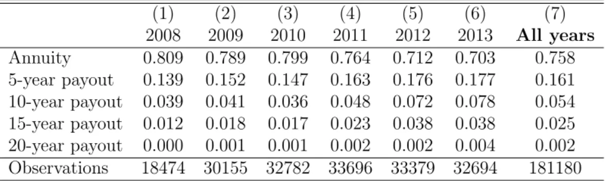
Table 3: Relative frequencies of the choice variable, reported by year (1) (2) (3) (4) (5) (6) (7) 2008 2009 2010 2011 2012 2013 All years Annuity 0.809 0.789 0.799 0.764 0.712 0.703 0.758 5-year payout 0.139 0.152 0.147 0.163 0.176 0.177 0.161 10-year payout 0.039 0.041 0.036 0.048 0.072 0.078 0.054 15-year payout 0.012 0.018 0.017 0.023 0.038 0.038 0.025 20-year payout 0.000 0.001 0.001 0.002 0.002 0.004 0.002 Observations 18474 30155 32782 33696 33379 32694 181180

This table shows relative frequencies of the choice variable reported by year (columns 1-6). Column 7 pools all years.

4.3

Payout choices (the dependent variable)

The payout choice variable is the outcome variable and takes on five different values as explained in section 2: individuals can withdraw their pension wealth over 5, 10, 15 or 20 years (fixed-term payouts) or as a life annuity.

Relative frequencies of the choice variable by year are reported in table 3. Between 2008, the year in which the ITP plan introduced fixed-term payouts, and 2013, the fraction of people that chooses the life annuity decreased from 80.9% to 70.3%. This averages to 75.8% over the whole period. The 5-year payout option is the most popular alternative among the fixed-term payouts. As seen in column (7), 16.1% of all retirees chose this option at retirement. However, the ten- and fifteen-year payout options have grown more in relative terms. The 10-year payout option, for example, was preferred by only 3.9% in 2008, but by 7.8% in 2013. Very few people (0.2%) choose the 20-year payout.

Table 4 reports relative frequencies of the choice variable by a number of individual characteristics. We see that the distribution of preferences vary substantially across some characteristics and less across others. In fact, differences in preferences for the payout options are significant along all characteristics in the table; all χ2_{-tests (not reported}

here) reject the null hypothesis that the distribution of preferences over the four possible options is independent of the different values of a characteristic.

There are large differences in payout preferences between income groups. 75.9% of the individuals in the bottom permanent income quartile choose the life annuity compared to 79.5% in the top quartile. Only 9.6% in the top quartile choose the 5-year payout, whereas 19.1% do so in the bottom quartile. Differences are even more pronounced across the account balance distribution. Only 66.7% in the bottom account balance quartile annuitize (27.3% choose the 5-year payout) compared to 84.7% in the top quartile (5.9% choose the 5-year payout). Individuals that continue to work after collecting the ITP benefit are more likely to annuitize than those who retire completely from the work force. Women choose the 5-year payout option more than men (18.7% vs. 14.4 %).

Individuals that die within two years of claiming are much more likely to choose the 5-year option, providing preliminary evidence of the presence of adverse selection. Annuitization rates are also somewhat higher among individuals with long-lived parents compared to individuals whose same-sex parent died before age 65.

5

Empirical Results

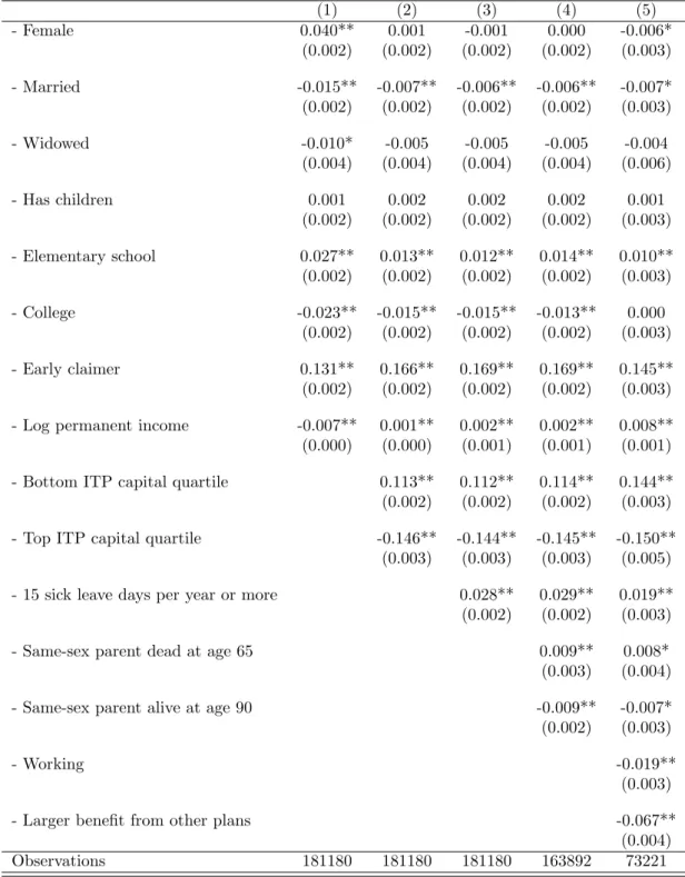
This section investigates the individual-level determinants of annuitization. It presents the results from a Multinomial Logit analysis applied to the pooled sample of individuals that claimed their ITP benefit between years 2008-2013. The reference category is the life annuity, which means that the marginal effect associated with each coefficient can be interpreted as the variable’s incremental effect on the probability of choosing payout op-tion K − 1 rather than the life annuity. The results for the fixed-term payout opop-tions are reported in separate tables. Table 5 and table 6 present the results for the 5- and 10-year payout respectively.28 _{The results for 15-year payouts are reported in the appendix.}29

28_{The demand for fixed-term payout options can also be estimated in an OLS framework. I estimate}

linear probability models where the dependent variable equals one if individual i chooses fixed-term payout option k and zero otherwise. The OLS estimates turn out to be very similar in magnitude to the marginal effects from the multinomial logit regressions and the inferences are unchanged.

Table 4: Relative frequencies of the choice variable, reported by demographic and socio-economic characteristics

Annuity 5-year 10-year 15-year Obs Female .747 .187 .0476 .0178 71,165 Male .766 .144 .0577 .0301 110,015 Has children .756 .16 .0555 .0268 135,348 No children .766 .163 .0486 .0209 45,832 Early retirement .543 .285 .107 .0545 22,248 Normal retirement age .788 .143 .0463 .0212 158,932 Working .833 .122 .0301 .0144 17,122 Not working .788 .154 .0406 .0165 64,289 Upper income quartile .795 .0962 .0589 .0447 45,028 Lower income quartile .759 .191 .0371 .0131 45,481 Upper pension capital quartile .847 .0586 .0412 .0485 44,364 Lower pension capital quartile .667 .273 .0515 .00901 46,934 Larger benefit from other plan .784 .171 .0325 .0114 16,252 Larger benefit from other plan .801 .141 .0399 .0172 65,159 15 sick leave days per year .735 .196 .0494 .0187 45,402 No sick leave .783 .133 .052 .0292 77,809 Mortality within 2 years .728 .236 .0261 .00944 1,800 Same-sex parent dead at age 65 .738 .172 .06 .0275 19,584 Same-sex parent alive at age 90 .767 .158 .0504 .0227 37,101 All individuals .758 .161 .0538 .0253 181,180

Note: This table reports relative frequencies of the choice variable by several demographic and socio-economic characteristics. The 20-year payout option is excluded because very few people choose this option.

I focus only on marginal effects to assess the quantitative impact of each explanatory variable because the estimated coefficients in the multinomial logit model reflect only the qualitative impact of an explanatory variable. A positive estimate of the marginal effect implies that the demand for the fixed-term payout option increases in that variable. Each specification includes a separate fixed effect for each year of claiming to control for variation in payout choices that is related to specific year effects. I also include a dummy for claiming before age 65 to control for variation in payout choices that is related to early retirement.30

Each column in table 5 and 6 report marginal effects from a separate regression. All specifications control for gender, marital status, the presence of children, education level, early retirement and log permanent income. The baseline observation is then defined as a single male with medium education (high school), no children and average permanent income who also retire at the normal retirement age (65). The results for this basic set of covariates are reported in column (1) in the respective tables. Specification (2) add two dummy variables for being in the top or bottom quartile of the ITP account bal-ance distribution to the basic set of control variables.31 Specification (3) and (4) include measures of health and parent mortality to assess the importance of adverse selection. Specification (5) also controls for non-ITP occupational pension benefits and whether the individual is working or not after retirement. This specification restricts the sample to claims made in or before year 2010, which is important to bear in mind when interpreting the results.

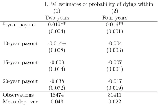
I also test for adverse selection by estimating linear probability models of whether re-tirees who claimed their ITP benefit at least two (four) years before the end of our sample period died within the first two (four) years after the claim date.32 _{Table 7 reports the}

results for these estimations.

Health, mortality and life exptectancy

The results with respect to health and life expectancy are broadly consistent with the predictions of life-cycle models. Column (3) and (4) of table 5 show that individuals with more than 15 sick leave days per year on average are 2.8 percentage points more likely to choose the 5-year payout option. The estimate is somewhat lower, but still significant when the sample is restricted to payout decisions made in 2010 or earlier (column (5)). The corresponding effect on the demand for the 10-year payout option is very close to zero, and even negative for the last specification, as seen in column (3)-(5) of table 6.

The estimated coefficients on same-sex parent mortality are significant and have the predicted signs. The marginal effect of same-sex parent mortality at age 65 on the prob-ability of choosing the 5-year payout option over the life annuity is 0.9 percentage points. Retirees whose same-sex parents was alive at age 90 decreases the demand for the 5-year payout by 0.9 percentage points. The corresponding effects for the 10-year payout are

30_{An alternative strategy to deal with age effects is to include a fixed effect for each year of age, but}

since almost 90% claim at age 65 a general dummy for early retirement seems sufficient.

31_{More specifically, the account balance distribution refers to the monetary value of the pension}

pay-ment under the life annuity. For each individual I observe the monthly benefit under the preferred payout option. The monetary value of the life annuity is then calculated as the product of the given retirement benefit and the relevant conversion factor. For example, if the monthly benefit under the 5-year payout is SEK 2000 and the conversion factor is 3.73, the value of the life annuity is equal to SEK 670.2 (2500 ÷ 3.73 = 670.2).

32_{Finkelstein and Poterba (2004) apply a similar LPM model framework as well as a hazard model}

Table 5: Results from Multinomial Logit regressions (marginal effects) - life annuity vs. 5-year payout (1) (2) (3) (4) (5) - Female 0.040** 0.001 -0.001 0.000 -0.006* (0.002) (0.002) (0.002) (0.002) (0.003) - Married -0.015** -0.007** -0.006** -0.006** -0.007* (0.002) (0.002) (0.002) (0.002) (0.003) - Widowed -0.010* -0.005 -0.005 -0.005 -0.004 (0.004) (0.004) (0.004) (0.004) (0.006) - Has children 0.001 0.002 0.002 0.002 0.001 (0.002) (0.002) (0.002) (0.002) (0.003) - Elementary school 0.027** 0.013** 0.012** 0.014** 0.010** (0.002) (0.002) (0.002) (0.002) (0.003) - College -0.023** -0.015** -0.015** -0.013** 0.000 (0.002) (0.002) (0.002) (0.002) (0.003) - Early claimer 0.131** 0.166** 0.169** 0.169** 0.145** (0.002) (0.002) (0.002) (0.002) (0.003)

- Log permanent income -0.007** 0.001** 0.002** 0.002** 0.008**

(0.000) (0.000) (0.001) (0.001) (0.001)

- Bottom ITP capital quartile 0.113** 0.112** 0.114** 0.144**

(0.002) (0.002) (0.002) (0.003)

- Top ITP capital quartile -0.146** -0.144** -0.145** -0.150**

(0.003) (0.003) (0.003) (0.005)

- 15 sick leave days per year or more 0.028** 0.029** 0.019**

(0.002) (0.002) (0.003)

- Same-sex parent dead at age 65 0.009** 0.008*

(0.003) (0.004)

- Same-sex parent alive at age 90 -0.009** -0.007*

(0.002) (0.003)

- Working -0.019**

(0.003)

- Larger benefit from other plans -0.067**

(0.004)

Observations 181180 181180 181180 163892 73221

Note: This table reports marginal effects estimated via multinomial logit. The marginal effect associated with each coefficient can be interpreted as the variable’s incremental effect on the probability of choosing 5-year payout rather than the life annuity. All specifications include year fixed-effects and a control for log permanent income. I include dummies to indicate whether the individual is female; is married; is widowed; has children; finished elementary school or college; retires before 65. Columns 2-5 also include dummies to indicate whether the individual belongs to the bottom or top quartile of the ITP pension income distribution. Column 5 also includes a dummy for having more than 15 sick leave days per year on average and column 6 dummies for same-sex parent mortality at age 65 and 90. Standard errors in parentheses. + Statistically significant at the 10 percent level. * Statistically significant at the 5 percent level. ** Statistically significant at the 1 percent level.

Table 6: Results from Multinomial Logit regressions (marginal effects) - life annuity vs. 10-year payout (1) (2) (3) (4) (5) - Female -0.006** -0.013** -0.013** -0.012** -0.015** (0.001) (0.001) (0.001) (0.001) (0.002) - Married 0.004** 0.005** 0.005** 0.004** 0.004* (0.001) (0.001) (0.001) (0.001) (0.002) - Widowed -0.005+ -0.004 -0.004 -0.005 -0.000 (0.003) (0.003) (0.003) (0.003) (0.004) - Has children 0.001 0.001 0.001 0.001 -0.000 (0.001) (0.001) (0.001) (0.001) (0.002) - Elementary school 0.002 -0.001 -0.001 -0.001 -0.004* (0.001) (0.001) (0.001) (0.001) (0.002) - College -0.009** -0.006** -0.006** -0.007** -0.001 (0.001) (0.001) (0.001) (0.001) (0.002) - Early claimer 0.044** 0.047** 0.047** 0.048** 0.037** (0.001) (0.001) (0.001) (0.001) (0.002)

- Log permanent income 0.004** 0.007** 0.007** 0.007** 0.006**

(0.000) (0.001) (0.001) (0.001) (0.001)

- Bottom ITP capital quartile 0.001 0.001 0.001 0.015**

(0.001) (0.001) (0.001) (0.002)

- Top ITP capital quartile -0.030** -0.030** -0.030** -0.021**

(0.001) (0.001) (0.002) (0.002)

- 15 sick leave days per year or more 0.001 0.001 -0.004*

(0.001) (0.001) (0.002)

- Same-sex parent dead at age 65 0.003+ 0.002

(0.002) (0.002)

- Same-sex parent alive at age 90 -0.003* -0.003+

(0.001) (0.002)

- Working -0.012**

(0.002)

- Larger benefit from other plans -0.019**

(0.002)

Observations 181180 181180 181180 163892 73221

Note: This table reports marginal effects estimated via multinomial logit. The marginal effect associated with each coefficient can be interpreted as the variable’s incremental effect on the probability of choosing the 10-year payout option rather than the life annuity. All specifications include year fixed-effects and a control for log permanent income. I include dummies to indicate whether the individual is female; is married; is widowed; has children; finished elementary school or college; retires before 65. Columns 2-5 also include dummies to indicate whether the individual belongs to the bottom or top quartile of the ITP pension income distribution. Column 5 also includes a dummy for having more than 15 sick leave days per year on average and column 6 dummies for same-sex parent mortality at age 65 and 90. Standard errors in parentheses. + Statistically significant at the 10 percent level. * Statistically significant at the 5 percent level. ** Statistically significant at the 1 percent level.

Table 7: Retiree mortality and payout choice

LPM estimates of probability of dying within:

(1) (2)

Two years Four years 5-year payout 0.019** 0.016** (0.004) (0.001) 10-year payout -0.014+ -0.004 (0.008) (0.003) 15-year payout -0.008 -0.007 (0.014) (0.004) 20-year payout -0.038 -0.017 (0.072) (0.019) Observations 18474 81411 Mean dep. var. 0.043 0.022

Note: Cols. 1 and 2 report estimates from a linear probability model of the probability of dying within two and four years of claiming, respectively. The excluded category is the life annuity. All regressions include, in addition to the covariates shown above, indicator variables for year of claiming and a dummy for claiming before age 65. Since mortality data is available only up to year 2012, the analyses on mortality within two and four years are restricted to individuals that claimed prior to year 2011 and 2009, respectively. Standard errors in parentheses. + Statistically significant at the 10 percent level. * Statistically significant at the 5 percent level. ** Statistically significant at the 1 percent level.

again smaller and amount to 0.3 and -0.3 percentage points, respectively.

The results from the linear probability model on ex-post mortality and payout choice also provide evidence pointing in the direction of adverse selection. Table 7 shows that individuals who choose the 5-year payout are 1.9 and 1.6 percentage points more likely to die within two and four years after claiming, respectively. This corresponds to per-centage effects of 42% and 73%. In contrast, there is no self-selection of individuals who die shortly after retirement into any of the other fixed-term payout options. If anything, mortality rates among retirees who choose 10-, 15- or 20-year payouts are lower than among annuitants.33 _{This results supports the general finding that individuals who enter}

retirement with low life expectancy or bad health tend to minimize the time period over which they withdraw their pension wealth.

Retirement wealth

As seen in table 5, adding controls for the size of the ITP benefit change the estimates of the basic set of covariates quite dramatically. Apart from the coefficient on early retire-ment, all coefficients become less significant, or even insignificant. The coefficient on log permanent income even changes sign across the model specifications. Column (1) reveals a negative relationship between permanent income and the probability of choosing the 5-year payout. The estimates reported in column (2)-(5), on the other hand, show that higher permanent income is associated with a marginally positive effect on the probability

33_{The estimates for the 20-year payout reflect remarkably low mortality rates. However, the coefficients}

of choosing the 5-year payout, given a certain level of retirement wealth. Because income is highly correlated with retirement wealth, it is difficult to evaluate the role of income when the model controls for the size of the pension benefit.

It is nevertheless clear that the size of the ITP benefit, or the account balance, is an important predictor of payout choice. Columns (2)-(4) in table 5 reveal that retirees in the bottom quartile of the account balance distribution are 10 percentage points more likely to choose the 5-year payout than those in the second and third quartile. Retirees in the top quartile, on the other hand, are 14-15 percentage points more likely to choose the life annuity on the margin.

The demand for 10-year payouts is less related to the size of the ITP benefit than the demand for 5-year payouts. The coefficients on the dummies for being in the bottom and top quartile reflect marginal effects of approximately 0.1 and -3.0 percentage points, respectively.

An alternative way to measure the impact of the size of the ITP benefit on the de-mand for fixed-term payouts is to replace the existing account balance dummies with the monetary value of the life annuity under each payout option. Again, the larger the annuity payment the lower the demand for the fixed-term payout options. The estimated coefficients (not reported here) are statistically significant and also economically mean-ingful with a one-standard deviation increase in the monthly life annuity payments (SEK 6216) decreasing the demand for the 5- and 10-year payout by 6.7 and 1.9 percentage points. B¨utler and Teppa (2007) also find that the marginal effect of pension wealth on the demand for life annuities is positive, but smaller than in this study. Chalmers and Reuter (2012), however, report that a one-standard-deviation increase in the life annuity payments increase the demand for the lump sum between 3.0 and 5.2 percentage points. Column (5) of tables 5 and 6 show that the demand for fixed-term payouts decrease when retirees receive income from some other occupational pension plan next to the ITP plan. More specifically, if at least 50% of the total occupational pension income is paid out from a non-ITP pension plan, the demand for the 5- and 10-year payout increases by 10.4 and 1.9 percentage points. This result contradicts the prediction that retirees that are less reliant on ITP benefits should be less likely to annuitize. A possible expla-nation to this results is that individuals with multiple sources of occupational pension devote more attention and effort to the payout decisions of other, more important pen-sion plans. The default option thus becomes particularly important for retirees that have contributed to different plans during their career. Note also that the magnitude of the coefficient on the bottom pension quartile becomes larger when we control for other oc-cupational pension income. This suggests that retirees that are located in the bottom quartile of the ITP account balance distribution because of low lifetime earnings are more likely to choose short payout periods than retirees who have small account balances because they spent large part of their careers working for employers outside the ITP plan. Bequest motives, socio-economic background and demographic characteristics I find no evidence of bequest motives having an effect on the payout decision. All coef-ficients on the presence of children in table 5 and 6 are close to zero and insignificant. Marital status also turns out to be an unimportant predictor of the payout decision. Column (1) in table 5 shows that married retirees are 1.5 percentage points less likely to choose the 5-year option. The effect becomes smaller in the augmented versions of the model that control for the size of the ITP benefit, parent mortality and health. Previous studies on the demand for life annuities have found significant and important effects of