SCHOOL OF EDUCATION, CULTURE AND COMMUNICATION
Bachelor Thesis in Mathematics/Applied Mathematics
Pricing American options using approximations by Kim integral equations
By Dmytro Sheludchenko Daria Novoderezhkina Mälardalen University Box 883 SE-721 23 Västerås Sweden Tel. +(46)21-10 13 00
SCHOOL OF EDUCATION, CULTURE AND COMMUNICATION
Bachelor thesis in mathematics / applied mathematics Date:
2011-06- Projectname:
Pricing American options using approximations by Kim integral equations Authors: Dmytro Sheludchenko Daria Novoderezhkina Supervisor: Anatoliy Malyarenko Examiner: Anatoliy Malyarenko Comprising: 15 points
ABSTRACT
The purpose of this thesis is to look into the difficulty of valuing American options, put as well as call, on an asset that pays continuous dividends. The authors are willing to demonstrate how mentioned above securities can be priced using a simple approximation of the Kim integral equations by quadrature formulas. Newton-Raphson iteration procedure is used in order to estimate the optimal exercise boundary for all time intervals. Method described above has proved to be a very efficient, accurate and fast in calculation numerical procedure. (Kallast, Kivinukk, 2003)
Last part of the report presents shortly a closed form valuation of American options based on the Petter Bjerksunds and Gunnar Stenslands model. The aim of this method rests in a logical approximation of American call and put options by means of dividing time to maturity into sub periods (similar to Kim’s approach) and applying a close to, however non-optimal option exercise strategy. As a result, a lower bound to the true option value is found. As Petter Bjerksund and Gunnar Stensland argue, the method is supposed to provide with a very accurate and highly computer efficient approximation of the true American option value. (Bjerksund, Stensland, 2002)
Finally, the results obtained by Bjerksund-Stenslands method are numerically compared by authors to the Kim’s. In Joon Kim’s approximation seems to be more accurate and closer to the chosen “true” value of an American option, however Bjerksund-Stenslands model is demonstrating a higher speed in calculations.
Key words: American options, early exercise boundary, optimal exercise, feasible non-optimal exercise strategy, integral equations, approximations, numerical procedures.
TABLE OF CONTENTS
Introduction ... 4
Kim equations in valuation of American put options ... 7
Approximate solutions of Kim equations ... 10
Calculating American Call Option Price Using Kim's Approximations ... 14
Short Description of Bjerksund-Stensland model ... 16
MATLAB Application’s Description and Analysis ... 19
Relationship between American option price and option parameters ... 21
Comparison with Binomial tree and Bjerksund-Stensland models ... 24
Conclusion ... 27
Introduction
Fischer Black and Myron Scholes in their paper “The pricing of options and corporate liabilities” have derived a theoretical closed-form valuation formula for pricing call and put options, however two of the restrictive assumptions that the authors used were: the options are of a European type and paying no dividends or other distributions. (Black, Scholes, 1973)
Definitions:
European-style options: are categorized as options that can only be exercised at one particular date, maturity date of the security. (Levy, Post, (2005), p.653)
American-style options: are described as instruments that can be exercised any time during options life. The holder of an American option has the opportunity to choose when the contract will be exercised, if ever; as long as it is before or on the security expiration date. (Levy, Post, (2005), p.653)
Robert Merton in 1973 has showed that options value is always greater, than the value it would have if it was exercised immediately. This means that a rational investor will wait to the maturity date to exercise his/her call option, which makes European and American call options have the same value. In his work Merton has also mentioned that American put option will enjoy a higher value than its European counterpart, this is due to possible advantageous exercise of the option before its expiration date. For example if the stock price falls dramatically and there is a little chance for it to exceed the exercise price before the option reaches its maturity, in this situation it is more beneficial to exercise the option immediately. The investor can save time and earn interest on the exercise price received up to the time when it would have been exercised otherwise. (Merton, 1973).
American options, for which an early exercise might be optimal, are written on many different commodities, commodity futures contracts and foreign currencies. American-style options’ early exercise premiums are implicitly incorporated in their prices. In comparison with European option-pricing issues; so far, unfortunately, there has been found no analytic
solution to the American option-pricing problems. (Barone-Adesi, Whaley, 1987) Since options traded on the international organized exchanges are in most cases American, it has been a lot studies that observe such an interest in their valuation problems and a desire to come up with the most efficient and effective method for their price calculation. (Kim, 1990, p 547-548) There has been mentioned above that Robert Merton managed to demonstrate that American call option will not be exercised early, as long as it won’t be an optimal decision, and therefore its value will coincide with the value of a European call option. However this statement had an important restricting assumption: the underlying asset for these options pays no dividends. (Merton, 1973) When the dividends are due, it can no longer be guaranteed that an American call option will not be exercised before its maturity. (Hull, (2006), p.219) Therefore the values of the American and European call options will differ in this case. If an underlying asset is entitled to distribute dividends and they are paid in a discrete manner, there exist analytical solutions for the calculation of the options price (Roll, 1977; Geske, 1979; Whaley, 1981). It might end up optimal to exercise an American call option that pays discrete dividends, prior to its expiration date; however in this case it has to be done immediately before ex-dividend date. It is not optimal to exercise a call any other time. (Hull, 2006)
Unfortunately, it is impossible to use this assumption in regard to American put options and calls written on foreign currencies and future contracts. Same can be said about options that have an underlying asset paying continuous dividends, as long as there is always a possibility of an early exercise during the life of an option. Therefore, we can conclude that European option pricing formulas are not applicable in this instance, and there exists no analytic solution to valuing American options written on foreign currencies and future contracts. (Kim, 1990).
The valuation of the American options is computationally challenging due to the fact that in order to proceed an optimal exercise boundary must be calculated as part of the solution. The methods applied in theoretical work can be divided into two groups: numerical and
approximation as it was done by Joon Kim (Kim, 1990) .When it comes to numerical methods, among the earliest and still excessively used are: the finite difference method of Brennan and Schwarts (1977) and the binomial tree model of Cox, Ross and Rubinstein (1979). These methods are considered relatively flexible, however very time consuming. The other group of methods, the approximation methods, are based on representations of
represented by option prices. According to Kallast and Kivinukk, This group of methods had been studied, among others, by: Geske and Johnson (1984), Bunch and Johnson (1992), Huang, Subrahmanyam and Yu (1996), Carr (1998) and Ju (1998). They represent analytic approximations and accuracy of the results improves with the increase in number of terms used. (Kallast, Kivinukk, 2003 p.362)
Methods implementing regression techniques to fit an analytical approximation based on lower and upper bounds of an American option, had been described by: Johnson (1983), Broadie and Detemple (1996). These methods require regression coefficients in order to be implemented, which in turn complicates the calculation; however they can be pretty fast. Among the fastest analytical approximations, MacMillans (1986) and Barone-Adesi and Whaleys (1987) can be underlined. Unfortunately, however, they are not the most accurate, especially in relation to long-term options. ( Ju, Zhong, 1999)
The aim of this paper is to present an analytic solution to pricing American options that are written on an asset paying continuous dividends and create MATLAB GUI application to present option prices to potential investors. We use a numerical approximation method for Kim (1990) equations with the help of quadrature formulas and Newton-Raphson iteration procedure. This approximation method seems to be very accurate and giving solutions to the Kim equations that are highly close to the chosen “true” values.
The rest of the thesis is structured in the following way. In chapter two Kim’s equations are described. Chapter three underlines approximate solutions of Kim’s equations by quadrature formulas. The first step is to find an early exercise boundary by applying the trapezoidal rule, followed by the Newton-Raphson iteration procedure to an integral equation. Once the boundary is calculated, the value of a selected American put option can be found with the help of Simpson’s rule. Following ideas were given by Siim Kallast and Andi Kivinukk (Kallast, Kivinukk, 2003).Chapter four demonstrates how an American call option value can be estimated using a very similar procedure to the one summarized above... Chapter five gives a short description of the Bjerksund-Stensland model. Chapter six provides readers with an insight to MATLAB applications description and analysis. The comparison between the results obtained using approximations of Kim integral equations and using Bjerksund-Stensland model, and those obtained by considering a binomial tree model with 10000 steps is presented and analyzed in the final chapter of our work.
Kim equations in valuation of American put options First, let us introduce the following notation:
– the price of an underlying asset at time , – the price of an underlying asset at time 0, – current time, – expiration date of the option, – strike price, – risk-free interest rate, – annualized volatility of the option, δ – a constant rate of continuous proportional
dividends, – the early exercise boundary of an American put, ) – the value of an American put. We will be considering American put option, written on the security that pays continuous dividends at a constant rate δ.
We will start by denoting the standard cumulative normal distribution function:
(1) And denoting: (2) (3)
We make an assumption that the early exercise boundary function is well-defined, unique and continuous with and . According to Kim (1990) this function is non-decreasing on the time interval from 0 to T. Also (Kim, 1990, p 560):
(4)
The value of American puts is governed by the following boundary conditions: (5)
(6)
(Kallast, Kivinukk, 2003, p 363)
By Black and Scholes (1973), the value of a European put can be expressed as the following equation:
(7) The value of an American put option at time 0 is, on the other hand, as follows (Kim, 1990, p 560): (8) Or (9) The equations above are demonstrating that the price of an American put option right now is equal to its European counterpart plus an early exercise premium in integral form. This premium can be treated as the value placed on the right to replace the European put with the American one.
According to Kim (1990), the early exercise boundary is the solution to the following integral equation: (10) (Kim, 1990, p 560) Or if we substitute:
It can easily noticed that equation (10) had been constructed from the right-hand side of
equation (8) and a boundary condition (6). The integration is performed on the time interval from to and the underlying asset price is being substituted by the early exercise boundary . (Kallast, Kivinukk, 2003, p 364)
Approximate solutions of Kim equations
Our task is to solve equations (8) and (10) by numerical approximation, in other words we are aiming to find a good approximation of the value of an American put option at time 0. Firstly we will derive the values of the early exercise boundary from equation (10). Then we will integrate equation (8), which in turn will allow us to achieve our goal in calculating options price. One of the most important steps in this procedure is the use of Newton-Raphson iteration in solving equation (10).
The interval of integration is divided into an even number of subintervals .
Subintervals [ti-1, ti] are of lengths . We will denote with . As long as coincides with , we obtain:
Let us denote:
(12) (13) Now Kim’s equations (8) and (10) can be expressed as follows:
(14)
(15)
BM can be easily computed with the help of formula mentioned earlier. We substitute for and for in equation (15) and obtain:
,B( (16)
We need to calculate the value of , however it seems complicated unless we use the trapezoidal rule:
The rest of the values of can also be found with assistance of the trapezoidal rule. For 0:
(18) The following limit contributes to calculation of ƒ( , ,0):
(19) Therefore, our equation becomes:
(20) From the equation listed above, it is possible to find numerical values of , by applying Newton-Raphson iteration procedure. First, lets rewrite equation (20) in the following way:
(21) According to Newton-Raphson iteration the values of ( ) can be represented through approximations of order , for
(22)
The first approximation will then be: = ( ). The value of is known to us by means of equation BM = K min(1, r/δ), therefore we are able to find with the help of equation (22) and keeping in mind that = . When the value of is successfully found, we repeat the same calculation procedure in order to obtain . The rest of the values ( , . . . , 0) are obtained following described above algorithm( (Kallast, Kivinukk, 2003, p 367).
(23)
In this case the function is the standard normal density function:
By graphing the early exercise boundary values { , investors are able to observe the shape of this boundary and see when an American put option can be exercised optimally (if the asset price falls below the early exercise boundary line, it is optimal to exercise put option).This will be also done in our MATLAB application.
Now we are ready to proceed to the final part in calculation of an American put option. Keeping in mind previously made assumption that is an even number of subintervals and applying the Simpson’s rule to the Kim equation (8), the value of American put at time 0 becomes:
(24) It had already been mentioned earlier that the function is a non-decreasing function, which means: for all t, and that is an optimal early exercise boundary below which it is optimal to exercise the given option. It follows, that as long as the underlying asset price stays lower or equals to , the price of an American put will be governed by the
following equation: . However, in case the stock price is higher, = 0 and can be found through equation (24):
(Kallast, Kivinukk, 2003, p 364-366)
Calculating American Call Option Price Using Kim's Approximations The idea and process of calculating American option price using Kim's integral equation is very similar to those for put option price. Algorithm for call option calculation was also presented by Siim Kallast and Andi Kivinukk (2003).
Now we denote as early exercise boundary for American option . Then we can follow the same process as in the previous section with some minor changes considering call option instead of put. As we already know, the value of American call option can be expressed as following:
(25) While early exercise boundary is a solution to following equation :
(26) Similarly to section 1 we can calculate value for
Let us denote:
Using the same arguments as in the part for put option calculating we can say that:
Solving equation (26) we can obtain following relationship for ,where :
(27)
Now if denote as x in (27) and move everything to the right hand side, we obtain a function . Our aim is to implement Newton-Raphson method to find all unknown values for In order to do it we need to know . can be expressed as :
Then using MATLAB we obtain values for . A comparison between the current stock price must be made in order to decide our further actions. In case :
Otherwise , we use following formula to calculate the price of American call option: (Kallast, Kivinukk, 2003, p 369)
Short Description of Bjerksund-Stensland model
The Bjerksund and Stensland (2002) model proposes to divide time to maturity interval into two parts. These parts have their own flat exercise boundary. All subsequent approximations are calculated by Genz algorithm since it is the only method that satisfies accuracy
requirements. The method was first proposed in 1993 and then modified by the authors in 2002. The method consists of numerous formulas that must be calculated to determine American option price.
Generally: Where and ; And denotes cost of carry rate :( ); -current stock price.
The function is calculated as : = ]
where ; (trigger prices ) are calculated as :
Where :
;
Function can be analytically represented: Where
(Haug, 2007,p 104-106).
Mathematical representation for this model provided above shows that it is relatively easy to implement the model using programming tools. This fact makes Bjerksund-Stensland model extremely compute efficient and convenient to program it.
MATLAB Application’s Description and Analysis
The main aim of our work is to provide potential investors with a computer program that computes American option prices using described above Kim’s method. In this section of our report we are going to describe and analyze MATLAB GUI application which implements Kim’s method and provides investor with price for American option with desired properties. At the start the program looks like this :
Figure 1:The main window of GUI application Kim’s Pricing Method.
.
Parameter Stock Price corresponds to variable in our theoretical part, Parameter Strike Price – to variable K. While Interest rate, Dividend yield ,Volatility and Maturity correspond to respectively. The last parameter (Number of desired time interval) is variable M. This parameter determines number of early exercises boundaries that are going to be calculated. With help of this parameter investor adjusts how precise the result going to be as well as investor can determine how often he or she is going to check if it is worthwhile to exercise the underlying American option. Default values for the parameters are displayed in the screenshot above.
Allowed values for the input parameters: Stock Price , Strike Price: These parameters can take any positive values.
Interest rate(in decimal form): Following parameter can take any economically reasonable values. For example, value 0 is not accepted as well as extremely high values like 0.5(50%). Value for this parameter must be realistic otherwise application either will not work or obtained results are highly unreliable.
Volatility(in decimal form): Value for this parameter must be positive and can take any values.
Maturity(in years): This parameter can take any positive values.
Dividend yield(in decimal form): The most important parameter in our case since its possible values are still subjected to debates in financial world. However, as it was mentioned above it is not optimal to exercise American call early . It is argued that it is not profitable to exercise American option on stock that does not offer dividends. This fact means that American option turns into European option whose value can be calculated using much easier approaches then Kim’s method. Thus we decided that the respective parameter should only take positive values.
Number of desired time interval: This parameter must take even positive values because of the reasons described in theoretical section.
If a user makes any mistake while writing parameters the application is going to inform him or her with a error warning.
After user have entered all parameters of American option, type of option in question can also be chosen with help of the menu to the left on picture 1. When option type is chosen , investor can choose which method should be used to calculate the option price by pressing respective button. Investor obtains also a graph on which relationship between calculated early exercise boundaries and time passed. A horizontal line on the graph represents ( current stock price). Using this graph investor can easily see when it is time to exercise the discussed American option .
Relationship between American option price and option parameters In this section we are going to investigate the relationship between American option prices and different option parameters like (
American option price and maturity
Figure 2. Option price and maturity.
The graph above represents the relationship that exists between option price and its option maturity. In order to investigate this relationship we calculated prices for call and put option using Kim’s method. We calculated call and put option prices for such parameters
And option maturity was changed in such way: .
As we can see from the graph both call and put prices grow as maturity increases. This is logical since options with longer maturities provide investor with more opportunities than the ones with shorter maturities. Thus price of such options must be higher.
0 5 10 15 20 25 0,5 1 1,5 2 2,5 3 3,5 4 4,5 5 Maturity Put Price Call Price
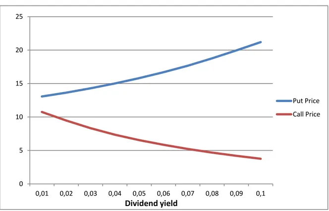
American option price and dividend yield
In this case we investigate relationship between option price and constant dividend yield that investor receives under options lifetime. This time we calculated put and call prices for options with such parameters:
We changed dividend yield in such a way :
The graph below portraits the existing relationship:
Figure 3. Option price and dividend yield.
As we can infer from the graph changes in dividend yield have different impacts on American put and call price. We see that put price increases as dividend yield increases while call price declines. The main reason for this is the fact that stock price generally declines when dividend payments are made. This means that higher constant dividend yield value (while other
parameters stay unchanged) suggests that there is a higher probability that the stock price is going to decline. Because of this more investors want to buy put option. Thus put option increases as dividend yield increases. Using similar arguments , the opposite is valid for call price. 0 5 10 15 20 25 0,01 0,02 0,03 0,04 0,05 0,06 0,07 0,08 0,09 0,1 Dividend yield Put Price Call Price
American option price and volatility
Relationship between American option price and stock volatility is similar to the relationship between American option price and maturity. Let us consider an American option with following parameters:
Consider
Using our application we can calculate respectively call and put option prices. Then if we plot them against values for volatility we obtain following graph:
Figure 4. Option price and volatility.
We can notice from the graph above that relationship between American option price and volatility has a lot in common with relationship between option price and maturity. Option price(despite option type) increases as security’s volatility increases . Explanation for this is that , as in the case with maturity, investor must pay extra for security that option of any type gives when security’s volatility is high.
American option price and risk -free interest rate
0 5 10 15 20 25 30 35 40 0,05 0,1 0,15 0,2 0,25 0,3 0,35 0,4 0,45 Volatility Put Price Call Price
In this case we investigate relationship between American option price and risk-free interest rate. In order to do it we consider an American option with following parameters:
And we change as
If we plot the obtained results for call and put we see that put price decreases as interest rate goes up and the opposite is valid for call price (see the graph below). This can be explained by that when interest rate is low since investors will rather buy put option (if difference between and is big enough) than invest in risk-free interest rates. In case of call option, we have opposite situation. Call price increases since investors are eager to rather buy call option ( because they are cheaper then stocks ) and invest funds they have left into risk-free rate.
Figure 5. Option price and risk-free interest rate.
Comparison with Binomial tree and Bjerksund-Stensland models In this section of our report we compare results for Kim’s method and B-S (Bjerksund-Stensland model) with the results for binomial tree for 10000 steps. We assume that these results are “real” prices for American option . The results for binomial tree model with 10000 time steps are taken from article by Kallast and Kivinukk (2003).
(Kallast,Kivinukk, (2003),p 381). 0 5 10 15 20 25 30 35 0,02 0,03 0,04 0,05 0,06 0,07 0,08 0,09 0,1 0,11 Interest rate Put Price Call Price
Let us consider an American put option with following parameters: . If we enter the mentioned parameters in our application and execute it :
Figure 6.Calculating American Put option price using applet Kim’s pricing method .
Result for an American option with such parameters for binomial tree model with 10000 steps is 22.2050. This results is very close to what we obtained using Kim’s method. However, we took rather low value for . If we increase value of investigated time intervals to 100
( ). We obtain that the option price in question is 22.2056. The last result equals almost the one for binomial tree model. If one wants to obtain even more closer
approximation, value must be increased. For example, option price with is 22.2053. We have obtained similar results for options with different parameters. Option prices are relatively different from the prices calculated with binomial tree model when value is rather low and converge to the results for binomial tree model with increase in .The value of parameter needed to obtain the same result as of the binomial tree model is less than 10000.
Judging from the performed analysis, we can say that Kim’s model is more efficient than binomial tree model in terms of time consumption and calculation easiness.
Comparison with Bjerksund-Stensland model
As we have mentioned in the dedicated part , Bjerksund-Stensland model provides a closed-form closed-formula for American option prices . Thus , this is very tempting to compare results obtained using Bjerksund-Stenslands model and Kim’s model. It is quite obvious that calculations with Bjerksund-Stenslands model are going to consume less time because of the described above property . In this section of our report we are going to compare results and speed of calculation for these two models.
Let us consider an American Put option with same parameters as in the previous section . As we already know (screenshot ) price calculated using Kim’s method is 22.226 ( and price using Bjerksund-Stensland method is 22.1197. By comparing these two results with the result for binomial tree model with 10000(option price is 22.2050) steps we discover that Kim’s model provides investor with more accurate option price. Now we take a look at computation speed in MATLAB for the two methods in question. By using MATLAB inbuilt functions we see that time required to make all necessary calculations for
Bjerksund-Stensland method is 0.0010 seconds while for Kim’s method 1.2353 seconds. Despite this fact, we can still argue that it is more preferable to use Kim’s method since the difference in calculation speed is relatively insignificant while Kim’s method gives more accurate
Conclusion
In this thesis we priced American call and put options using approximations by Kim integral equations. The application of Newton-Raphsons iteration procedure played a highly
significant role in estimating the optimal early exercise boundary values. MATLAB, the program used for creating graphical support and performing the calculations standing behind the results of this report; as well as characteristics of the required input parameters have been described and analyzed in detail. The relationships between an American option price and input parameters have been discussed and graphically demonstrated. A brief description of the Bjerksund-Stensland model had been given along with the comparison between the obtained results through Kim’s method with the ones provided by the Bjerksund-Stenslands approach. The selected “true” value for American option is represented by the price obtained by means of the Binomial tree model with 10000 steps. Kim’s method had provided surprisingly accurate results in a quite short period of time. With the number of time subintervals ( ) big enough, options price equals the chosen “true” value. Bjerksund-Stensland model is also quite effective, however not to the same extend as Kim’s. Even though Bjerksund and Stensland provided us with the option price calculation procedure that works faster than Kim’s, we are still leaning in our preference towards approximation by Kim’s integral equations. The main reason being – it is much more accurate and the difference in calculation times between the two methods is not substantial enough to discourage us from using Kim’s approach.
List of References
1. Barone-Adesi, G. and Whaley, R. (1987) Efficient analytical approximation of American option values, Journal of Finance 42, 301–320.
2. Bjerksund P., Stensland G. (1993); Closed Form Approximation of American Options, Scandinavian Journal of Management 9, 87–99.
3. Black, F. and Scholes, M. (1973) The pricing of options and corporate liabilities, Journal of Political Economy 81, 637–659.
4. Brennan, M. and Schwartz, E. (1977) The valuation of American put options, Journal of Finance 32, 449–462.
5. Broadie, M. and Detemple, J. (1996) American option valuation: New bounds,
approximations, and a comparison of existing methods, Review of Financial Studies 9, 1211–1250.
6. Bunch, D. & Johnson, H. (1992) ’A Simple and Numerically Efficient Valuation Method
7. for American Puts Using a Modified Geske–Johnson Approach’, Journal of Finance
47, 2, 809–816.
8. Carr, P. (1998) Randomization and the American put, Review of Financial Studies 11, 597-626.
9. Cox, J. C., Ross, S. A., and Rubinstein, M. (1979) Option pricing: A simplified approach, Journal of Financial Economics 7, 229–264.
10. Geske R. (1979); A Note on an Analytical Formula for Unprotected American Call Options on Stocks with known Dividends, Journal of Financial Economics 7, 63–81. 11. Geske, R. and Johnson, H. E. (1984) The American put valued analytically, Journal of
Finance 39, 1511–1524.
12. Haug,E.G.(2007), The Complete Guide to Option pricing formulas(second edition) ,McGraw-Hill.
13. Huang, J., Subrahmanyam,M., and Yu, G. (1996) Pricing and hedging American options: A recursive integration method, Review of Financial Studies 9, 277–300. 14. Hull, J. C. (2000) Options, Futures, and Other Derivatives, Prentice-Hall
International, Inc.
15. Johnson, H. (1983) ’An Analytical Approximation for the American Put Price’, Journal of Financial and Quantitative Analysis 18, 141–148.
16. Ju, N. (1998) Pricing an American option by approximating its early exercise
boundary as a multipiece exponential function, Review of Financial Studies 11, 627– 646.
17. Ju, N., & Zhong, R. (1999). An approximate formula for pricing American options. Journal of Derivatives, 7, 31–40.
18. Kallast, S., & Kivinukk, A. (2003). Pricing and hedging American options using approximations by Kim integral equations. Review of Finance, 7, 361–383.
19. Kim, I. J. (1990) The analytical valuation of American options, Review of Financial Studies 3, 547–572.
20. Levy, H.,& Post T. (2005) Investments, Financial Times Prentice-Hall. 21. MacMillan, L. (1986) ’Analytic Approximation for the American Put Option’,
Advances in Futures and Options Research 1, 119–139.
22. Merton, R. C. (1973) ’Theory of Rational Option Pricing’, Bell J. Econ. Management Sci. 4, 141–183.
23. Roll, R. (1977), "A critique of the asset pricing theory's tests Part I: On past and potential testability of the theory", Journal of Financial Economics 4 (2): 129–176 24. Whaley, R. E. (1981), “A Note on an Analytical Formula for Unproteced American
Call Options on Stocks with Known Dividends.” Journal of Financial Economics 7, 207-211.