User cost estimation on road networks by means of bayesian probabilistic networks

USER COST ESTIMATION ON ROAD NETWORKS

BY MEANS OF BAYESIAN PROBABILISTIC NETWORKS

Markus Deublein

Swiss Federal Institute of Technology, Infrastructure Management Group

CH-8095 ZURICH Switzerland E-mail: deublein@ibi.baug.ethz.ch

Bryan T. Adey

Swiss Federal Institute of Technology, Infrastructure Management Group

CH-8095 ZURICH Switzerland E-mail: adey@ibi.baug.ethz.ch

ABSTRACT

In this paper a methodology for the development of multiple impact models for road networks is described. Road impacts can be categorized into impacts for different stakeholder groups, namely the public, the owner and the road users. The current investigations address multiple impacts only for road users, but the developed methodology can be extended to estimate the impacts of all stakeholder groups. Impacts for road users are differentiated into costs due to travelling time, vehicle operation and accident injuries. The accident and injury costs are assessed based on multivariate regression analysis and Bayesian Probabilistic Networks. The proposed methodology for the assessment of road user impacts is different from existing impact models since uncertainties are incorporated into the model. Accordingly, all variables of the model are represented probabilistically.

To demonstrate the usefulness of the methodology, models were developed for the prediction of multiple road user impacts on three road segments that were different in terms of traffic configurations, road designs and surface conditions. Based on the assumptions made for the model development, the results show that accident and injury costs represent only a small share of the total user impacts.

An important feature of the introduced methodology for road impact assessment is that it provides decision support, e.g. on how to optimally allocate budgets into accident risk reducing interventions and evaluate the portfolio of changeable measures in terms of their effect on the accident risk before and after they are implemented.

1 INTRODUCTION

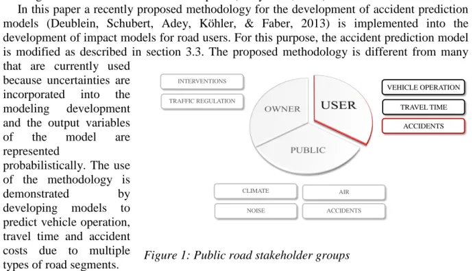
Optimal intervention strategies are those that result in the lowest negative impacts for stakeholders which for public roads can be grouped as the owner, the user, and the public (Figure 1) (Adey et al., 2012). The determination of optimal intervention strategies on road segments, including when to intervene, the type of intervention to execute and the traffic configuration to use during the intervention is the main goal of road owners with the largest impacts on road users. Although it is acknowledged that impacts on the stakeholder groups “owner” and “public” including e.g. environmental impacts are very important contributors to

the entire impacts caused by a road network, this paper – as a preliminary investigation – solely focusses on the estimation of road user impacts, namely impacts due to travel time costs, vehicle operation costs and accident costs.

The estimation of these impacts is tremendously difficult due to the many different and interconnecting physical relationships. For instance, the increase in travel time due to deteriorating road condition depends on the slope, the curvature, the capacity, and the speed limit of the road as well as the number of vehicles travelling on the road. At the same time, the number of vehicles and the road condition have amongst other variables an influence on the occurrence probabilities of accident events.

Estimations of impacts and assumptions of physical relationships are at least partly subject to uncertainties. These uncertainties can broadly be categorized into aleatory (natural variability of the phenomenon itself) and epistemic uncertainties (modeling uncertainty, statistical uncertainty) (M. H. Faber & Stewart, 2003) and are so far not considered in the existing studies for evaluation of road impacts (Adey et al., 2012).

In this paper a recently proposed methodology for the development of accident prediction models (Deublein, Schubert, Adey, Köhler, & Faber, 2013) is implemented into the development of impact models for road users. For this purpose, the accident prediction model is modified as described in section 3.3. The proposed methodology is different from many that are currently used

because uncertainties are incorporated into the modeling development and the output variables of the model are represented

probabilistically. The use of the methodology is

demonstrated by developing models to

predict vehicle operation, travel time and accident costs due to multiple types of road segments.

2 METHODOLOGY

2.1 General

The described methodology uses accident prediction models based on multivariate Poisson-Lognormal regression analysis and Bayesian Probabilistic Networks (BPNs).

BPNs are directed acyclic graphs containing chance nodes which represent variables either as continuous random variables or as sets of discrete states, where each state represents an interval. The nodes are connected through directed arrows representing the causal dependencies between variables. BPNs were originally developed in the field of artificial intelligence approximately 30 years ago, but are now widely used in the field of engineering (Michael H. Faber, 2003). They are used to compactly represent the joint probability density

TRAVEL TIME VEHICLE OPERATION ACCIDENTS NOISE CLIMATE AIR TRAFFIC REGULATION INTERVENTIONS ACCIDENTS

function of all variables in the model. The outcomes of the compilation of the BPN are the marginal probability distributions of the model response variables, i.e. the distributions of the different impact types.

The structure of a BPN is described by using family relations. If node A is directly linked to node B then the node A is denoted as the parent node of the child node B. The joint probability distributions of all nodes are calculated by multiplying the conditional probabilities of the child nodes with their parent nodes. The marginal probabilities of the child nodes are calculated by summing the joint probabilities of all possible states. When the value of one or more variables is observed, referred to as evidence in BPN terminology, the prior probability distributions of the remaining variables can easily be updated. The Bayesian approach necessitates that a prior (conditional) probability mass is assigned for each node. The prior probability represents the existing knowledge before any (new) evidence in terms of data is available (Box & Tiao, 1992). The adequate choice of the prior distributions is very much dependent on the investigated problem and the availability of information (Gelman, Carlin, Stern, & Rubin, 2004). A more detailed description of BPNs is given in Jensen & Nielsen (2007), Bayraktarli (2009) and Schubert (2011).

2.2 Modeling Steps

The modeling approach can be sub-divided into five consecutive steps. The first three steps are to determine the indicator variables (Step 1), the intermediate variables (Step 2) and the response variables (Step 3) to be included in the BPN and the corresponding prior probabilities of each node. The indicator variables, e.g. road design parameters, surface conditions and traffic characteristics, are the input variables (parent nodes) of the BPN. The intermediate variables (intermediate nodes) are defined to establish a network structure which a) is capable of representing the functional relationships to be used and b) ensures at the same time that the conditional probability tables of the child nodes do not become too large and, therefore, computational expensive. The intermediate nodes are child nodes of the indicator variables and become parent nodes of the response variables. The response variables are the variables, with which it is desired to have information, e.g. accident costs.

Step 4 is to construct the BPN and Step 5 is to enter the values of the indicator variables (evidences) for the road segments to be investigated and compile.

3 MODEL DEVELOPMENT

3.1 Step 1: Determine Indicator Variables

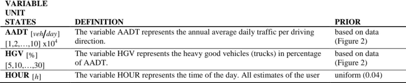
The definitions, prior probability assumptions and the states of the BPN nodes for the indicator variables are given in Table 1.

Table 1: Indicator Variables: Definitions, prior assumptions and node states

VARIABLE UNIT

STATES DEFINITION PRIOR

AADT [veh day]

[1,2,…,10] x104

The variable AADT represents the annual average daily traffic per driving direction.

based on data (Figure 2)

HGV [%]

[5,10,…,30]

The variable HGV represents the heavy good vehicles (trucks) in percentage of AADT.

based on data (Figure 2)

VARIABLE UNIT

STATES DEFINITION PRIOR

[0,1,…,23] costs are made for one specific hour of the day.

TVC [ ]−

[A,B,C,D,E,F]

The variable TVC represents different traffic variation curves in percentages of AADT with given HOUR. Six different TVCs are distinguished having different traffic configurations and quantities. E.g. TVC (A) in Figure 3 has a clear peak of traffic volume (rush hour) at 7am with apercentage of 12.5% of the AADT.

(Pinkofsky, 2005) (Figure 3)

LAN [ ]−

[1,2,3,4]

The variable LAN represents the number of lanes per driving direction. based on data (Figure 2)

SPDsig [km h/ ]

[60,70,…,130]

The variable SPDsig represents the signalized speed limit. based on data (Figure 2)

CUR [ ]−

[0,2,…,10]

The variable CUR represents the horizontal curvature of the road. It is defined as an integer variable having values between zero (straight road) and ten (very high curvature). CUR is determined as the fraction of the sum of the length of ten subsequent 50m road sections, divided by the length of the straight connection between the starting point of the first section and the end point of the tenth section.

based on data (Figure 2)

GRD [%]

[-6,-4,-2,0,2,4,6]

The variable GRD represents the percentage of upwards or downwards longitudinal gradient.

based on data (Figure 2)

WZ [ ]−

[1=no,2=yes]

The variable WZ represents the presence of Work Zones. Within work zones, specific accident risk increasing variables might be present, which are currently not included in the model, e.g. reduced lane width, distraction, soiled pavement. Different studies show that the crash rates increase when work zones are introduced (Ha & Nemeth, 1995; Khattak, Khattak, & Council, 2002; Rophail, Zhao, Yang, & Fazio, 1988; Wang, Hughes, & Council, 1996). For the current investigations the accident costs within work zones are assumed to be increased by 25%.

assumption: ( 1) 0.9 ( 2) 0.1 p WZ p WZ = = = = I2 and I4 [ ]− [0.5,1,…5]

The variables I2 and I4 represent the road pavement conditions. In Switzerland, the pavement conditions are measured using six indices according to VSS SN 640 925b. Increasing values of the indices indicate decreasing road conditions. For the assessment of road user impacts the following two indices are relevant:

I2 = index for longitudinal unevenness; I4 = index for skid resistance; The prior probabilities are determined assuming a Gamma distribution assuming that the road conditions have in average I2- and I4-values of

3

I

x = with a standard deviation of sI= (Figure 4). 2

assumption: Γ(α=2.25,β=1.33)

Γ(α,β) abbreviates the Gamma distribution with parameters α (shape) and β (scale).

In Figure 2 the (prior) relative frequencies of the indicator variables are shown for which data was available. The prior probabilities of the indicator variables for which no data was available are modelled either based on assumptions or based on literature information.

Figure 2: Prior probabilities based on data used in Deublein et al. (2013)

Figure 3: Traffic variation curves (Pinkofsky, 2005)

Figure 4: Prior probabilities for the states of I2 and I4 (assumption of Gamma distribution)

3.2 Step 2: Determine Intermediate Variables

The intermediate variables of the BPN are illustrated by the grey shaded nodes in Figure 10. The intermediate variables are introduced into the BPN to represent the complex functional relationships between the model input (risk indicating variables) and the model output (model response variables). The data for all injury accidents together with the corresponding numbers of injured road users (LIN, SIN, FAT, Table 2) is the same as in the case study described in Deublein et al. (2013). In case the injury could not be assigned to one of the injury levels, injuries “with unknowable magnitude” were merged to the group of severe injuries. Mass accidents (>10 vehicles being involved at one accident site) were excluded from the dataset. Additionally, injury accidents which were caused by drivers who were under the influence of alcohol were not taken into account, as well as data which had no clear specification of the

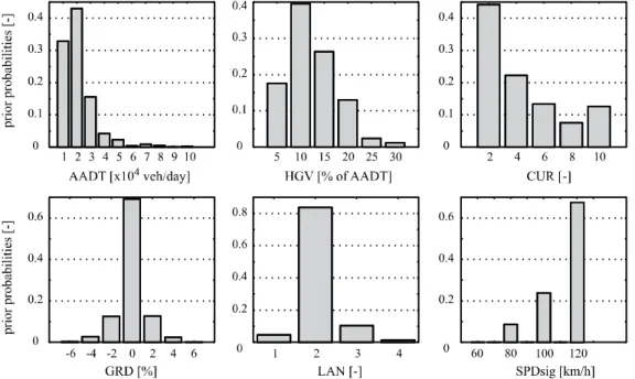
location or could not be allocated to one of the driving directions. In Table 2 definitions, prior model assumptions and states of the intermediate nodes are listed.

Table 2: Intermediate model variables

VARIABLE UNIT

STATES DEFINITION PRIOR

LOS

[ ]−

[A,B,C,D,E,F]

The variable LOS represents the level of service. It indicates the quality of the traffic flow. LOS depends on the number of lanes and boundary values for the maximum number of vehicles per hour on a road segment. The boundary values used to define the LOS are taken from FGSV (2001). Polynomial functions were adapted to the values for LAN=1 to LAN=3 in order to extrapolate the boundaries to roads with LAN=4 per driving direction (Figure 5).

deterministic A = free flow

B = reasonably free flow C = stable flow

D = pending unstable flow E = unstable flow F = breakdown flow

VEHph

[veh h ]

[0.5,1,…,10]x103

The variable VEHph represents the vehicles per hour on a considered road segment. The traffic volume per hour during the day is assessed as the fraction of the AADT given the type of TVC for a specific hour of the day (HOUR).

assumption:

( _VEHph, _VEHph)

truncN µ σ bounds (0,10’000)

VEHph AADT TVC HOUR

µ = ⋅ 0.05 VEHph VEHph σ = ⋅µ SPDact [km h ] [5,10,…,150]

The variable SPDact represents the actual driving speed. Given information about SPDsig and LOS, the SPDact is assumed to be normal distributed with mean value derived by establishing polynomial functions under two constraints: (a) if LOS=A then

SPDact LOS SPDsig

µ = and

(b) if LOS=F then _{5 /}

SPDact LOS km h

µ = .

The resulting polynomial functions are given in Figure 6. The standard deviation of SPDact is assessed by fitting a

polynomial function to observed deviation from the signalized speed limit (Figure 7).

assumption: ( SPDact, SPDact) truncN µ σ bounds (0,150) ( ) SPDact f LOS µ = ( ) SPDact f SPDsig σ = AMFI4 [ ]− [1,1.02,…,2]

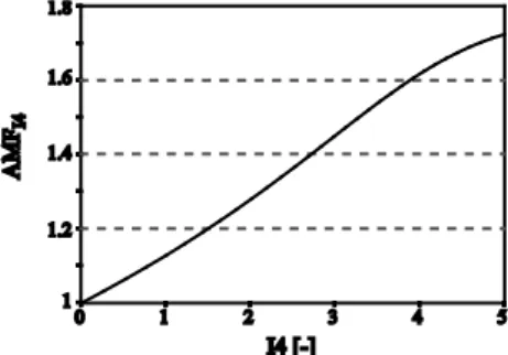
The variable AMFI4 represents the accident modification factor related to surface friction index I4. The functional relationship between AMFI4 and I4 is given in Figure 8 assessed based on the equations provided in Adey et al. (2012). The AMFI4 is representing the relative change in the expected number of injury events given changes in the surface friction (I4) compared to the assumed base condition of I4=0 (new constructed/replaced pavement).

assumption: ( , ) I4 I4 AMF AMF N µ σ ( ) I4 AMF f I4 µ = 0.05 I4 AMF σ = AMFS [ ]− [0.05,0.1,…,1.8]

The variable AMFS represents the accident modification factor related to SPDact. The functional relationships between the SPDact and the AMFS are based on the power-functions given in Nilsson (2004).

The AMFS is representing the relative change in the expected number of injury events given changes in the driving speed (SPDact) with respect to the base condition of the driving speed which is assumed to be SPDbase=100 km/h (assumed average driving speed on Swiss rural motorways).

assumption: ( , ) S S AMF AMF N µ σ S AMF SPDact SPDbase µ = 0.1 S AMF σ = LINr [LIN mvk] [0.02,0.04,…,2]

The variable LINr represents the occurrence rate of lightly injured road users per million vehicle kilometer (mvk) and year. A road user is considered to be lightly injured if the damage to his well-being lasts less than 25 days following the accident.

The rates of lightly injured road users are determined based on the accident prediction methodology given in (Deublein, et al., 2013).

SINr

[SIN mvk] [0.002,0.004,…,0.2]

The variable SINr represents the occurrence rate of severely injured road users per mvk and year. A road user is

considered to be severely injured if the damage to his well-being lasts more than 24 days following the accident.

The rates of severely injured road users are determined based on the accident prediction methodology given in (Deublein, et al., 2013).

FATr

[FAT mvk]

The variable FATr represents the rate of fatally injured road users per mvk and year. A road user is fatally injured when he

the rates of fataly injured road users are determined based on the accident

VARIABLE UNIT

STATES DEFINITION PRIOR

[0.002,0.004,…,0.2] has died within 30 days following the accident event as a consequence of accident induced injuries.

prediction methodology given in (Deublein, et al., 2013). LINe [ ]− [0.05,0.1,…1] and ]1,2,...,20]

The variable LINe represents the expected number of light injured road users per homogenous segment. LINe is calculated by multiplying the LINr with AMFI4 and with AMFS 2 (Nilsson, 2004). assumption: ( LINe, LINe) truncN µ σ bounds (0,20) 6 2 10 ... LINe HS I4 S

LINr length VEHph

AMF AMF µ = ⋅ ⋅ ⋅ ⋅ ⋅ 0.1 LINe LINe σ = ⋅µ SINe [ ]− [0.005,0.01,…,0.1] and ]0.1,0.2,...,2]

The variable SINe represents the expected number of severely injured road users per homogenous segment. SINe is calculated by multiplying the SINr with AMFI4 and with AMFS3 (Nilsson, 2004). assumption: ( SINe, SINe) truncN µ σ bounds (0,2) 6 3 10 ... SINe HS I4 S

SINr length VEHph

AMF AMF µ = ⋅ ⋅ ⋅ ⋅ ⋅ 0.1 SINe SINe σ = ⋅µ FATe [ ]− [0.005,0.01,…,0.1] and ]0.1,0.2,...,2]

The variable FATe represents the expected number of fatally injured road users per homogenous segment. FATe is calculated by multiplying the FATr with AMFI4 and with AMFS 4 (Nilsson, 2004). assumption: ( _FATe, _FATe) truncN µ σ bounds (0,2) 6 4 10 ... FATe HS I4 S

FATr length VEHph

AMF AMF µ = ⋅ ⋅ ⋅ ⋅ ⋅ 0.1 FATe FATe σ = ⋅µ LIN [mu h km( ⋅ )] [2,4,…,100] and ]0.1,0.2,…,5] x103 and ]5,6,…,20] x103

The variable LIN represents the costs for lightly injured road users. Taking into account the information provided by the Highway Safety Manual (AASHTO, 2010), the costs in Swiss

Francs (CHF) per lightly injured road user are assumed to

correspond to UCLIN=58 ' 400 [CHF].

assumption:

( _LIN, _LIN)

truncN µ σ bounds

(0,20’000)

LIN LINe UCLIN WZ

µ = ⋅ ⋅ 0.1 LIN LIN σ = ⋅µ SIN [mu h km( ⋅ )] [2,4,…,100] and ]0.1,0.2,…,5] x103 and ]5,6,…,20] x103

The variable SIN represents the costs for severely injured road users. Taking into account the information provided by the Highway Safety Manual (AASHTO, 2010), the costs per severely injured road user are assumed to correspond to

203'700 [ ] SIN UC = CHF . assumption: ( _SIN, _SIN) truncN µ σ bounds (0,20’000)

SIN SINe UCSIN WZ

µ = ⋅ ⋅ 0.1 SIN SIN σ = ⋅µ FAT [mu h km( ⋅ )] [2,4,…,100] and ]0.1,0.2,…,5] x103 and ]5,6,…,15] x103 and ]15,20,…,140] x103

The variable FAT represents costs for fatally injured road users on the homogeneous segment. Taking into account the information provided by the Highway Safety Manual (AASHTO, 2010), the costs pro fatally injured road user are assumed to correspond to _UCFAT =_{3'780 ' 400 [CHF]}.

assumption:

( FAT, FAT)

truncN µ σ bounds

(0,140’000)

FAT LINe UCFAT WZ

µ = ⋅ ⋅ 0.1 FAT FAT σ = ⋅µ TIM [ ]h [0.01,0.02,…,0.25]

The variable TIM represents the travelling time per km given information about SPDact and I2. TT is assessed in

accordance with Adey et al. (2012) where a penalty factor increases TT on a road segment as a function of the longitudinal unevenness (I2).

Values needed for the assessment of TT are assumed to be a=2.3, b=2 and c=0.6 (Adey, et al., 2012).

deterministic HS l tt SPDtech = where min( , ) SPDtech= SPDr SPDact I2 b SPDsig a for I2 b SPDr c SPDsig for I2 b − − ⋅ ≥ = < HR [mu h] [0.1,0.2,…,1] x103 and ]1,2,…,10] x103

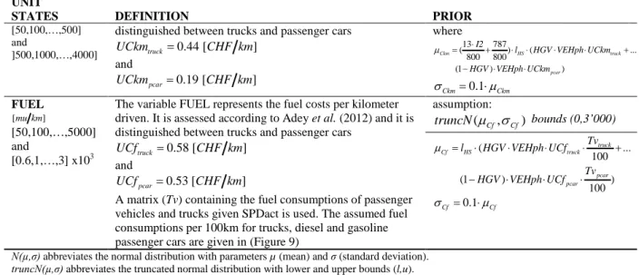
The variable HR represents the vehicle costs per hour driven. It is assessed according to Adey et al. (2012) and it is distinguished between trucks and passenger cars

6.16 [ ] truck UCh = CHF h and 1.91 [ ] pcar UCh = CHF h assumption: ( Ch, Ch) truncN µ σ bounds (0,10’000) ( ... (1 ) ) Ch HS truck pcar tt l HGV VEHph UCh HGV VEHph UCh µ = ⋅ ⋅ ⋅ ⋅ + − ⋅ ⋅ and σ_Ch=0.1⋅µ_Ch KM [mu km]

The variable KM represents the vehicle costs per kilometer driven. It is assessed according to Adey et al. (2012) and it is

assumption: ( _Ckm, _Ckm)

VARIABLE UNIT

STATES DEFINITION PRIOR

[50,100,…,500] and

]500,1000,…,4000]

distinguished between trucks and passenger cars

0.44 [ ] truck UCkm = CHF km and 0.19 [ ] pcar UCkm = CHF km where 13 787 ( ) ( ... 800 800 (1 ) ) Ckm HS truck pcar I2 l HGV VEHph UCkm HGV VEHph UCkm µ = ⋅ + ⋅ ⋅ ⋅ ⋅ + − ⋅ ⋅ 0.1 Ckm Ckm σ = ⋅µ FUEL [mu km] [50,100,…,5000] and [0.6,1,…,3] x103

The variable FUEL represents the fuel costs per kilometer driven. It is assessed according to Adey et al. (2012) and it is distinguished between trucks and passenger cars

0.58 [ ] truck UCf = CHF km and 0.53 [ ] pcar UCf = CHF km

A matrix (Tv) containing the fuel consumptions of passenger vehicles and trucks given SPDact is used. The assumed fuel consumptions per 100km for trucks, diesel and gasoline passenger cars are given in (Figure 9)

assumption: ( _Cf, _Cf) truncN µ σ bounds (0,3’000) ( ... 100 (1 ) ) 100 truck Cf HS truck pcar pcar Tv l HGV VEHph UCf Tv HGV VEHph UCf µ = ⋅ ⋅ ⋅ ⋅ + − ⋅ ⋅ ⋅ 0.1 Cf Cf σ = ⋅µ

N(µ,σ) abbreviates the normal distribution with parameters µ (mean) and σ (standard deviation). truncN(µ,σ) abbreviates the truncated normal distribution with lower and upper bounds (l,u).

Figure 5: Maximum road capacities (VEHph) for the different number of lanes (LAN) defining the different levels of service (LOS=A-F) (FGSV, 2001)

Figure 6: Actual driving speed (SPDact) for different signalized speed limits (SPDsig=60-130) as a polynomial function of LOS (assumption)

Figure 7: Standard deviation of the actual driving speed (SPDact) given signalized speed limits (SPDsig) (based on data used in (Deublein, et al., 2013))

Figure 8: Accident modification factor

(AMFI4) given road surface friction index (I4)

(Adey, et al., 2012)

Figure 9: Fuel consumption given actual driving speed (SPDact) (Keller & Zbinden, 2004)

3.3 Step 3: Determine Response Variables

The response variables are the three different user cost variables, namely the travelling time costs (TT), the vehicle maintenance and operation costs (VO) and the accident costs (AC). The definitions, modelling assumptions and states of the response variables are given in Table 3.

Table 3: Model response variables

VARIABLE UNIT

STATES DEFINITION PRIOR

TT [mu h km( ⋅ )]

[0.1,0.2,…,2] x103 and

[5,10,…,90] x103

The variable TT represents the travelling time costs. They are due to time which is lost during travelling on the road section. TT varies indirectly as a function of pavement condition represented by the longitudinal unevenness index I2.

The unit costs for TT are _{30.93 [ ( )]}

TT

UC = CHF veh h⋅ , assuming an

occupancy rate of 1.57 persons per car (Adey, et al., 2012).

assumption: ( TT, TT) truncN µ σ bounds (0,90’000) where TT tt VEHph UCTT µ = ⋅ ⋅ 0.15 TT TT σ = ⋅µ VO [mu h km( ⋅ )] [0.1,0.2,…,2] x103 and [4,6,…,24] x103

The variable VO represents the costs of maintenance and operation of a vehicle. Vehicle maintenance comprises man-hours needed for maintenance work and material costs. Vehicle operation costs include additionally costs for fuel consumption.

assumption: ( VO, VO) truncN µ σ bounds (0,24’000) where VO Ch Ckm Cf µ = + + 0.1 VO VO σ = ⋅µ AC [mu h km( ⋅ )] [2,4,…,50] and [60,70,…,200] and ]0.3,0.4,…,2] x103

The variable AC represents the costs of road users suffering different injury levels which are caused by accidents on the road section. The total amount of user costs due to injuries is represented by the sum of the costs resulting from the different injury severities. Accidents with property damage only (PDOs) are neglected since the expected costs for such damages are very low compared to the costs arising due to injuries.

assumption:

( AC, AC)

truncN µ σ

bounds (0,2’000)

where

AC LIN SIN FAT

µ = + +

0.1

AC AC

σ = ⋅µ

N(µ,σ) abbreviates the normal distribution with parameters µ (mean) and σ (standard deviation). truncN(µ,σ) abbreviates the truncated normal distribution with lower and upper bounds (l,u).

3.4 Step 4: Develop model

The development of the impact model is based on observable risk indicating variables (model input) and predicted model response variables (model output). Additionally, intermediate variables are introduced to simplify the structure and the computation processes of the model.

The different variables are represented in the BPN as nodes. The nodes are connected by means of arrows which represent the functional relationships between the variables as given in the Tables 1-3. The functional relationships are determined empirically based on available data or are defined based on theoretical assumptions.

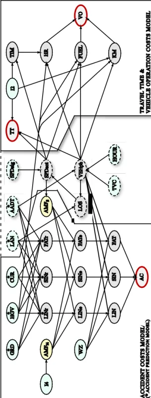
The entire BPN can be described as two sub-models (Figure 10). The first sub-model consists of the model response variables travel time costs (TT) and vehicle operation costs (VO) and the corresponding indicator and intermediate variables. The second sub-model consists of the response variable accident costs (AC) and represents the user costs due to injuries caused by accidents on the road segments. It contains an accident prediction model, that is developed based on the methodology described in Deublein et al. (2013) and uses data-based multivariate Poisson-Lognormal regression analysis and Bayesian updating algorithms to establish the internal relationships between its nodes and the predictive distribution functions of the injury occurrence rates (LINr, SINr and FATr). The variables which were used as input variables for the accident prediction model are indicated by the small stars in the nodes (Figure 10). The difference between the prediction model developed here and that proposed in Deublein et al. (2013), is that the signalized speed limit is only used to determine the crash modification factor AMFS. The AMFS is used because previous case studies have

revealed that the signalized speed limit on rural motorways shows only very small variation. Hence, using the signalized speed limit directly as indicator variable for the injury occurrence rates would result in a rather weak relationship between the signalized speed limit and the different injury occurrence rates.

An additional AMF is introduced to represent the influence of the indicator for skid resistance (I4) on the occurrence probabilities of injury events caused by road accidents, AMFI4. The skid resistance of the road surface is considered to have influence on the braking

distance of vehicles which can be a decisive factor for the emergence of accidents.

The two sub-models are connected by indicator variables and intermediate variables that are used as input variables for both sub-models. These ‘connecting’ variables are indicated by the dashed lines of the nodes LAN, AADT, SPDsig, SPDact, LOS, VEHph, TVC and HOUR. For example, as illustrated in Figure 10, when evidence is given for the node SPDsig the change in the signalized speed limit will change the probabilities in the states of the child node SPDact (being additionally dependent on LOS). The change in the node SPDact in turn influences all sub-models for accident costs, travel time costs and vehicle operation costs.

Each node in the network contains a probability mass function over the defined range of states. A conditional probability table is associated with each node that contains the conditional probabilities for each state of the node given the states of the other nodes. The values of all variables were represented as being in one of a reasonable number of discrete states.

The total impact for road users on a road network is obtained by summing the costs predicted for the three response variables (nodes with bold, red lines) using the two sub-models.

3.5 Step 5: Enter values of

indicator variables and

compile

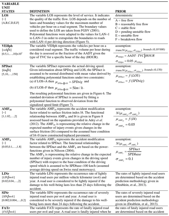
In order to evaluate the methodology, it is used to develop models to predict vehicle operating costs, travel time costs and accident costs for three different types of road segments. The three fictive road segments (HS1, HS2, HS3) are independent and represent three different road designs and traffic densities, i.e. the traffic volume or traffic flow on one HS has no influence on the other HSs and the individual HSs can be spatially separated. The values of all investigated variables are considered to be the same within each HS. The road segments are assumed to be representative of typical highway segments on the Austrian highway network for which substantial data is available (Deublein, et al., 2013). The values of the indicator variables for the three different HS to be entered into the BPN are given in Table 4.

HS1 is a 2-laned motorway section in good condition (I2 = 1, I4 = 1) (definitions according to Table 1). The TVC=C represents a relative constant traffic flow during daytime (Figure 3).

Figure 10: Developed Bayesian Probabilistic Network for estimation of the total road user costs including the sub-models for travelling time (TT), vehicle operation (VO) and accident injuries (AC)

The average daily traffic is moderate with 30’000 vehicles per day of which 20% are heavy good vehicles. The signalized speed limit is 130km/h. The user cost models are developed for the hour between 10am and 11am.

HS2 is a 3-laned motorway section in medium condition (I2 = 3, I4 = 3). The traffic is assumed to vary on this road segment significantly over the course of the day, e.g. due to additional traffic going into a city in the morning (TVC=A). The average daily traffic is 70’000 vehicles per day of which 30% are heavy good vehicles. The signalized speed limit is 100 km/h. The user cost models are developed for the hour between 10am and 11am.

HS3 is essentially the same motorway section as HS2, but during the execution of an intervention, where the number of lanes has been reduced from 3 to 1, and the signalized speed limit is reduced from 100 to 60km/h. The road condition state on to which the vehicles are being deviated is poor (I2 = 4, I4 = 4).

The user cost models are developed for the hour between 7am and 8am being the hour over the course of the day with the highest percentage of the traffic volume. The hour between 7am and 8am was chosen for this segment as the lowest level of service (LOS = F – breakdown flow / congestion) occurs then as opposed to the hour between 10am and 11am.

The values of the indicator variables (Table 4) are entered in the BPN and it is

compiled. The marginal probability

distribution functions are calculated using the inference engine as implemented in the software packages of e.g. Hugin (Hugin,

2008) or GeNie

(Decision-Systems-Laboratory-Pittsburgh, 2006).

4 RESULTS

The expected values E

[ ]

[ ]

Francs (CHF) per km and hour. The response variables of the developed impact models

facilitate the representation of the uncertainties which are connected to the data used for model development and to the model itself. The results provided in Table 5 indicate that the traffic volume, the number of lanes and the signalized speed limit have considerable influence on the values of the impact types. When the road condition is in relatively good condition (best three of five condition states), the vehicle operation costs comprise the largest share of the impacts. When the road condition is in poor condition (worst two of five condition states) the travel time costs comprise the largest share of the impacts. The extremely high values for travel time costs when the road is in the worst condition state is due to the fact that the traffic flowing on the road segment is close to the maximum capacity of the road segment, and congestion is occurring. The accident impacts represent only a very small share of the total user costs. The highest values for injury costs are obtained on HS1 triggered by the high signalized speed limit due to the applied power functions (Nilsson, 2004). In case the traffic

Table 4: Values of indicator variables for HS1, HS2 and HS3 Variables [Unit] HS1 HS2 HS 3 length [km] 1 1 1 time [h] 1 1 1 AADT [veh/d ay] 30’0 00 70’0 00 70’ 000 HGV [%] 20 30 30 LAN [-] 2 3 1 CUR [-] 0 0 0 GRD [%] 0 0 0 TVC [-] C A A HOUR [h] 11a m 11a m 8a m WZ [-] no no yes SPDsig [km/h] 130 100 60 I2 [-] 1 3 4 I4 [-] 1 3 4

flow is congested (as it is on HS3) only very few injury causing accidents are expected to occur.

Table 5: Values of the response variables - expected user costs in [CHF km h( ⋅ )]

HS1 HS2 HS3

E[.] STD[.] COV E[.] STD[.] COV E[.] STD[.] COV

TT 540.57 279.64 0.52 1’380.59 1’091.13 0.79 41’948.21 7’762.63 0.19

VO 1‘053.39 176.70 0.17 1‘524.64 231.97 0.15 6‘341.95 982.47 0.15

AC 37.44 26.91 0.72 19.28 10.44 0.54 28.56 6.07 0.21

total 1’631.49 244.08 0.15 2’924.14 558.55 0.19 48’318.72 8’921.19 0.18

The COV varies considerably between different road segments and response variables. The lowest values of the COV (and hence, the lowest dispersion in the estimates of the user costs) are observed on the road section HS3. For vehicle operation costs the COV is almost constant on the three considered road segments and for injury costs it decreases with decreasing speed limits and decreasing levels of service.

The discretized marginal probability distributions of the TT, VO and AC response variables are shown for the three different road segments (Figure 11).

5 CONCLUSIONS

A methodology based on Bayesian probabilistic networks was presented to develop models to be used to predict multiple impacts of road segments, namely travel time costs, vehicle operation costs and accident injury costs. The methodology allows taking into account all uncertainties which are connected to the assumptions of physical models or functional relationships used for model development. The developed models can be easily updated when additional data for the same problem becomes available, or when it is desired to use the models for a new but similar problem (e.g. to predict impacts in different countries with different road conditions, driving behaviors, etc.). To demonstrate the methodology, models were developed for the prediction of impacts on three road segments that were different in terms of traffic configurations, road designs and surface conditions.

Through this example it can be seen that the proposed methodology can be used to simultaneously estimate impacts on road segments taking into consideration the complex relationships between them. The practical implication of the methodology is that the developed models can be used as supportive instruments for risk based decision making, i.e. for determining optimal intervention strategies by assessing and evaluating the impacts of different intervention alternatives. It is believed that this ability will yield decision makers substantial benefits as they try to determine optimal intervention strategies for highway networks in terms of saved time and increased accuracy with respect to how estimations are currently made.

It has to be discussed that road impact modeling in general requires numerous assumptions to be made for the implemented model variables. In the current investigations, assumptions were made in regard to the distribution families and distribution parameters of the random variables. These assumptions can be based either on empirical investigations, theoretical suppositions or on experts’ experiences. Once assumptions are made, it is difficult to judge whether these assumptions are reasonable or not, unless the predictions can be compared to real observations.

REFERENCES

AASHTO. (2010). Highway Safety Manual (Vol. Volume 2). Washington, DC: American Association of State Highway and Transportation Officials, AASHTO

Adey, B. T., Herrmann, T., Tsafatinos, K., Lüking, J., Schindele, N., & Hajdin, R. (2012). Methodology and base cost models to determine the total benefits of preservation interventions on road sections in Switzerland. Structure and Infrastructure Engineering, 8(7), 639-654. doi:

10.1080/15732479.2010.491119

Bayraktarli, Y. Y. (2009). Construction and Application of Bayesian Probabilistic Networks for Earthquake Risk

Management. Doctor of Sciences Dissertation, Swiss Federal Institute of Technology Zurich, Zürich.

Retrieved from http://e-collection.ethbib.ethz.ch/view/eth:969

Box, G. E. P., & Tiao, G. C. (1992). Bayesian inference in statistical analysis (Wiley Classics Library Edition Pubulished 1992 ed.). New York: John Wiley.

Decision-Systems-Laboratory-Pittsburgh. (2006). Genie 2.0 (Version 2.0). Pittsburgh, USA: Decision Systems Laboratory, http://dsl.sis.pitt.edu. Retrieved from http://genie.sis.pitt.edu/about.html

Deublein, M., Schubert, M., Adey, B. T., Köhler, J., & Faber, M. H. (2013). Prediction of road accidents: A Bayesian hierarchical approach. Accident Analysis & Prevention, 51(0), 274-291.

Faber, M. H. (2003, June 8-13, 2003). Uncertainty Modeling and Probabilities in Engineering Decision

Analysis. Paper presented at the Proceedings OMAE2003, 22nd International Conference on Offshore

Mechanics and Arctic Engineering, Cancun, Mexico.

Faber, M. H., & Stewart, M. G. (2003). Risk assessment for civil engineering facilities: critical overview and discussion. Reliability Engineering & System Safety, 80(2), 173-184. doi:

FGSV. (2001). Handbuch für die Bemessung von Strassenverkehrsanlagen. Köln: Forschungsgesellschaft für Strassen- und Verkehrswesen.

Gelman, A., Carlin, J. B., Stern, H. S., & Rubin, D. B. (2004). Bayesian data analysis Boca Raton: Chapman & Hall/CRC.

Ha, T., & Nemeth, Z. (1995). Detailed study of accident experience in construction and maintenance zones.

Transportation Research Record, 1509.

Hugin. (2008). Hugin Researcher (Version 6.904). Aalborg: Hugin Experts A/S. Retrieved from www.hugin.com

Jensen, F. V., & Nielsen, T. D. (2007). Bayesian networks and decision graphs (2nd ed.). New York, NY: Springer.

Keller, M., & Zbinden, R. (2004). Air destroying material emissions of road traffic Environmental Series. Switzerland: Federal Authority for the Environment, Forests and Country.

Khattak, A. J., Khattak, A. J., & Council, F. M. (2002). Effects of work zone presence on injury and non-injury crashes. Accident Analysis & Prevention, 34, 19-29.

Nilsson, G. (2004). Traffic Safety Dimensions and the Power Model to Describe the Effect of Speed on Safety. PhD, Lund Institute of Technology, Lund. (Bulletin 221)

Pinkofsky, L. (2005). Typisierung von Ganglinien der Verkehrsstärke und ihre Eignung zur Modellierung der

Verkehrsnachfrage. PhD, Technical University Braunschweig, Braunschweig.

Rophail, N., Zhao, M., Yang, S., & Fazio, J. (1988). Comparative study of short- and long-term urban freeway work zones. Transportation Research Record, 1163.

Schubert, M., Hoj, N. P., Kohler, J., & Faber, M. H. (2011). Development of a best practice methodology for risk assessment in road tunnels (pp. 157): ASTRA, Federal Road Office, Switzerland, research report 1351. Wang, J., Hughes, W. E., & Council, F. M. (1996). Investigation of highway work zone crashes: What we know