Estimating the income elasticity of demand for international air travel

(1)

Master’s thesis • 30 credits

Environmental Economics and Management- Master's Programme Degree project/SLU, Department of Economics, 1230 • ISSN 1401-4084 Uppsala, Sweden 2019

Estimating the Income Elasticity of Demand

for International Air Travel

-the Financial Crisis and its Effect on Irish

Income

(2)

Swedish University of Agricultural Sciences

Faculty Of Natural Resources and Agricultural Sciences Department of Economics

Estimating the Income Elasticity of Demand for International Air

Travel- the Financial Crisis and its Effect on Irish Income

Connor Craig

Supervisor: Rob Hart, Swedish University of Agricultural Sciences, Department of Economics

Assistant supervisor: Jonathan Stråle, Swedish University of Agricultural Sciences, Department of Economics

Examiner: Jens Rommel, Swedish University of Agricultural Sciences, Department of Economics Credits: Level: Course title: Course code: Programme/education: 30 credits A2E

Master thesis in Economics EX0905

Environmental Economics and Management Master's Programme 120,0 hec

Course coordinating department: Department of Economics Place of publication: Year of publication: Title of series: Part number: ISSN: Uppsala 2019

Degree project/SLU, Department of Economics 1230

1401-4084

Online publication: http://stud.epsilon.slu.se

Key words: income elasticity, international air travel demand, financial crisis, natural experiment

(3)

iii

Abstract

During the 2008 financial crisis, aggregate income along with the number of air travellers in Ireland both decreased significantly. This thesis aims to estimate the income elasticity of demand for international air travel in Ireland using a difference-in-differences instrumental variables model (DID/IV), where Norway is used as a control group and the financial crisis serves as an exogenous instrument for a change in income. Using this exogenous variation caused by the crisis as an instrumental variable for the effect of income on international passenger numbers generates income elasticity estimates of between 4.645 to 9.310. This implies that a 1% change in income leads to a 4.645% to 9.310% change in the demand for international air travel. Assuming that aggregate incomes are rising over time, then the findings of this study suggest that international air passenger numbers will increase significantly. This will have important implications for policymakers aiming to reduce the future amount of carbon emissions being released into the Earth’s atmosphere.

(4)

(5)

v

List of figures

1. Effect of the financial crisis on consumer budget constraint 7 2. International air transport to EU countries for Ireland and Norway 11

3. Standardized real GDP 12

(7)

vii

List of tables

1. Average number of international passengers, Difference-in-differences 2004-2011 12

2. Baseline estimates 19

3. Reduced form estimates 21

4. Second stage estimates 22

5. Experimenting with different “crisis” years 25

6. Leads and lags 26

7. Leads and Lags test - using individual quarters from 2005 up until 2012 35 8. Experimenting with different income variable 37

(8)

(9)

1

1. Introduction

There is a growing interest among market participants and governments alike to understand how income influences consumer demand for air travel. Assuming that aggregate incomes are gradually increasing over time, a positive income elasticity of demand for air travel would imply that the number of passengers will be increasing. Studies like Chi and Baek (2013), Marazzo et al. (2010) and Hakim and Merkert (2017) point out that this could have important implications for numerous reasons, with the most notable relating to the issue of pollution. If the number of air passengers is increasing in line with incomes, then this will increase the amount of carbon emissions being released in the future. Policymakers aiming to reduce global 𝐶𝑂₂ emissions associated with air travel will greatly benefit from having access to robust income elasticity estimates in order to assess the magnitude of these future emission levels, and consequently tailor their policies to best achieve the desired reductions. Airline companies and aircraft manufacturers also have a vested interest in passenger demand forecast models in order to predict passenger travel behaviour and expected future passenger numbers. If passenger numbers are increasing, then manufacturers will have to increase the production of new airplanes, and airlines will have to consider opening new or increased travel routes. Accurate demand forecasts are also of significant importance when planning infrastructure development required to satisfy future demand. Airports, for example, rely on this information with regards to determining the number of car parking spaces, the size of terminal buildings, and ensuring that there is appropriate accommodation close by, all of which should be adjusted to meet future demand (Paul et al, 2017).

The general objective of this paper is thus to estimate the income elasticity of demand for international air travel, which will allow for predictions over the future number of international air passengers. In order for this to be achieved, I aim to exploit the abrupt fall in aggregate income experienced in Ireland as a result of the 2008 financial crisis. Using this event as an exogenous shock to income in the country should allow for the possibility to extract the exogenous variation in income, which will then permit this paper to estimate the unbiased impact of a change in income on the demand for international air travel.

One of the main limitations of many previous studies such as Paul et al. (2017) and Chi and Baek (2012) is that they use standard methods like ordinary least squares (OLS) or fixed effect models to estimate the income elasticity of air travel. The limitation of these approaches is that they can often suffer from endogeneity issues, such as the main explanatory variable and the dependent variable both influencing each other. This will mean that the explanatory variable is related to the error term which will lead to biased estimates. The issue of reverse causality between the income and passenger number variables, is a common problem in the field of income elasticity estimates for air travel, which almost none of the previous studies have addressed. This paper uses a difference-in-differences instrumental variables approach (DID/IV) similar to Duflo (2001) in order to correct for this issue. This involves using the

(10)

2

variation in income caused by the financial crisis as an exogenous instrument for the impact of income on the demand for international air travel. Using this method, a difference-in-differences analysis is conducted in order to measure the effect that the financial crisis had on Ireland’s aggregate income compared to a control group Norway, which was much more sheltered from the effects of the crisis. This study argues that the financial crisis is an appropriate instrument to use for this study since it satisfies the required assumptions for a valid instrument, namely that it clearly had a significant impact on income in Ireland, however it should have no direct effect on the number of passengers, except through income. Additionally, since the crisis was an exogenous event, where it largely came by surprise, then it should be unrelated to the error term in the standard OLS model. This should mean that any change in passenger numbers should be the result solely of a change in income rather than some omitted variable.

Using this method, I estimate a positive income elasticity of demand of between 4 and 10, meaning that a 1% increase in income will lead up to a 10% increase in the demand for air travel. This would suggest that consumers demand for air travel reacts much more aggressively as a result of a change in income than prior estimates would recommend. It also implies that the future number of air passengers will be increasing at a much higher rate than most previous studies would indicate.

There are however a number of issues that should be considered when interpreting the results of this study. In order for the findings to be valid it should be the case that the control group Norway, was unaffected by the crisis. Additionally, using the crisis as an instrument means that it should only affect passenger number through the explanatory variable income, and not through other factors such as expectations about the future. These, along with a few smaller problems, are issues that need to be addressed in this paper before drawing any concrete conclusions based on this study’s results.

The remaining sections in this paper are organised as follows. In section 2, a brief background relating to the political and institutional set up in both countries is presented. This is done to explain why Ireland suffered so much more from the crisis than did Norway. In section 3, I briefly outline previous attempts and methods used to calculate income elasticity for air travel, whilst pointing out the limitations, before laying out some theoretical framework in section 4. Next in section 5, I describe the data being used and present graphically the income and passenger trends in the two countries. Section 6 presents the methodology and section 7 outlines the reduced form equation along with the DID/IV set up. I then present the main results in section 8 before carrying out some robustness and sensitivity checks in section 9. Finally, section 10 will consist of the main discussion and limitation of this study, followed by the conclusion in section 11.

(11)

3

2. Background

2.1. The financial crisis in Ireland

Although the 2008 banking crisis in Ireland was made worse by the global financial crisis, the reasons which led to its occurrence were mainly domestic. During the mid-1990’s right through till the late 2000’s, Ireland experienced one of its largest periods of economic growth. This period, which became known as the “Celtic tiger”, saw Irelands economy expand at an average rate of roughly 9.4% per year throughout the 1990’s (The Economist, 2004). Foreign borrowing rose rapidly from €15 billion to well over €100 billion in 2008 (Independent, 2012). This period of economic expansion was more akin to what some of the Asian countries had experienced during the 19th_{century but was something that had rarely been seen in Europe before. By the}

end of the Celtic tiger’s reign, Irelands GDP per capita exceeded that of every European nation bar Luxemburg.

This boom period incentivised banks to increase their lending’s and investment practices so much so that by 2007 mortgage debt within the country increased to around 36% of total private sector debt. Irish banks were lending money to almost anyone and everyone who was interesting in buying or building a house. This led to a huge real-estate bubble and a consequent upward spike in house prices. During this period the Irish government had already been running a huge budget deficit in order to keep the economy going, and by 2009 this deficit had reached a value of 14.3% of the country’s GDP, the largest in the EU for that year (RTE, 2010). When the boom period finally ended in 2008 house prices began to plummet, and in some instances, homeowners found themselves in a position where they owed the bank more than two or three times the value of their home. Unsurprisingly, large masses of people soon began to default, and the banks were stuck in a position of desperate cash shortages and an ever-increasing amount of unpaid debts. Soon the Government was forced to step in and bail these banks out however at a period where global markets where in disarray over the effects from the 2008 financial crisis, international banks had stopped lending and thus available funds to help ease the country’s financial woes had dried up. As a result, in 2009 Ireland became the first country in the Eurozone to enter into a recession. Fast forward two years later to the height of the financial crash, where the country’s respective banking and housing markets had both completely collapsed, Ireland was forced to accept a whopping €67.5 billion EU-IMF bailout package, of which it was still paying back as of when this report was written (Irish Times, 2017). Thus, when looking for factors which explain why Ireland was hit so much harder by the financial crisis in 2008 than were other nations, it was evidently a result of inadequate risk management practices within the Irish banks coupled with poor regulation and supervision of these companies by the Irish Government and financial regulators at the time (Kennedy and O’Sullivan, 2010). The skyrocketing unemployment levels and mortgage defaults, brought

(12)

4

about by the crisis, led to most of the population living on low or medium incomes, drastically cutting back on their spending.

2.2. Norway’s insurance strategy

In Norway the situation in 2008 was much different. The financial crisis had caused almost every country in the developed world’s economies to come staggering to a halt however, Norway was one of the few exceptions. The country’s GDP over the period actually grew by a few percentage points and the unemployment rate was kept down below 3.5%, which was the lowest in Europe at the time (Thomas, 2009). The country even used $175 billion out of their sovereign wealth fund to purchase stocks during the global downturn when markets were still in the midst of a severe crash (Guo, 2010). These statistics pose the question as to how Norway was able to achieve such a feat whilst most of its European counterparts were struggling. Well first and foremost the Norwegian banking sector had a more cautious approach to lending and borrowing than much of the rest of Europe and America. Norwegian banks purchased a very low amount of sub-prime based bonds and a result did not suffer the same ramifications once this market began to collapse. This coupled with the low presence of UK and US banks in the country, who were two of the largest sellers of such loans, separated Norway somewhat from the rest of the world when the economic markets began to crash.

Furthermore, capital requirements by the Norwegian financial supervisory authority (FSA), a government agency whose job is to supervise financial companies within the country, were higher in Norway than they were for much of the rest of Europe, with banks required to hold at least 7% in cash holdings. Banking supervision in the country was also significantly strengthened, especially after the crisis of the 1990’s. Supervisors were appointed to conduct regular audits of large and medium sized banks, and if a bank was found to have a significantly higher risk of default than normal then specific capital requirements were swiftly imposed. Finally, strong public finances coupled with large revenues from the country’s oil and gas reserves allowed the government to stimulate the economy during the early stages of the crisis and invest in new projects to create jobs, thus lessening the impact of the global recession (Skogstad Aamo, 2018). As a result, the Norwegian people’s expenditure was much less affected than it was in Ireland.

3. Previous literature

Throughout the previous literature there exists a wide range of studies carried out with the intention of determining which factors most influence the demand for air travel. However, the percentage of these studies focusing specifically on incomes direct effect on demand is much scarcer. Over the past number of years there has been an increase in such studies, yet the majority of these are carried out using largely similar approaches.

(13)

5

Earlier studies relied heavily on static OLS models to examine the relationship between aggregate income and air transport demand. Ba-Fail et al. (2000) for example, use a number of standard OLS models in order to forecast demand for domestic air travel in the kingdom of Saudi Arabia. They find a positive correlation between domestic air travel expansion and income growth in the region. However, most of the models used in their study suffered from severe multicollinearity which impeded forecasters ability to draw inferences about the significance of individual variables in the model. Additionally, this multicollinearity caused estimators to have significantly high variances, thus making it difficult to interpret any meaningful conclusions from the results.

Paul et al. (2017), also use a standard OLS method to test five different explanatory variables influence on the demand for air travel in order to display which factors drive demand the most. They look at population size and age structure, urban agglomeration, education status and GDP per country, as the main explanatory factors. Using data from 28 European countries, the authors find that income, tertiary education and the geography of a country are the key drivers of demand. This study however only uses data for 2014 and thus admits that further studies would benefit from using panel data so as to consider the developments over time. For this paper I use a panel data set in order to account for such developments.

More recent studies have attempted to extend the analysis of income elasticity to medium and low-income countries, since most prior research has focused only on high-income countries. Using a dynamic panel data model, Valdez (2014) finds that income is the most important determinant for air travel in middle income countries, where income growth accounts for roughly 75% of passenger traffic growth compared to somewhere between 40% and 50% for high income countries. Hakim and Merkert (2017) examine the determinants of air travel in South Asian countries using a fixed effects model with data ranging over 43 years. They find that income has an over proportionate effect on passenger demand and a slightly less, but still positive, effect on air cargo. Given that GDP is growing rapidly in this region, the findings of this study suggests that the anticipated increase in disposable income will lead to an “explosion” in air passenger demand along with considerable growth in the air freight industry. This will only be possible however if local infrastructure is invested heavily in so that it will be capable of handling this imminent growth. Given that my study is looking at Ireland and Norway, which are both highly developed countries, then according to Valdez (2014) and Hakim and Merkert (2017) it would be expected that income should play a slightly lesser role in determining air passenger numbers here than it would for developing countries.

Finally, the Bureau of Transport and Communications Economics (BOTACE) carried out a study where they disaggregated existing models to examine demand more precisely across markets. This updated approach enabled the authors to determine individuals demands per country and also by purpose of travel. This kind of disaggregation, which allows for the analysis of the unique features of individual markets, is rare throughout previous literature. The authors calculated income elasticity estimates across multiple different markets and the results were all positive, although they ranged from inelastic to highly elastic. They found that, for example, the income elasticities for travelling from Australia to Korea and Taiwan were 5.9 and 11.58 respectively. These highly elastic estimates differed substantially from markets like

(14)

6

the UK, which was determined to have an income elasticity of only 1.03, indicating that routes travelling to this destination were much less elastic to changes in incomes. The study also found that elasticities often significantly differed depending on passenger types in addition to the origin-destination market (BOTACE, 1995).

What is surprising when going through previous studies is how little effort has been made to calculate the income elasticity of demand using only an exogenous variation in income. This would allow to control for many endogeneity issues arising from reverse causality or omitted variable bias. One of the few studies that have dealt with the issue of reverse causality is from Chang and Chang (2009). However, this study is not conducted in the context of aggregate income’s effect on passenger demand for air travel, but rather it’s impact on air cargo expansion. Given that air cargo expansion tends to lead to higher trade which thus increases GDP, then it would be expected that causation will run in this direction. However economic development may lead consumers to buy more foreign goods which would increase imports and consequently air cargo will increase. Thus, in this case the direction of causality between these two variables is unclear. In this study the authors carry out a granger causality test, as a simple and effective approach to detect the presence of any causal relationship between the two variables, and in which direction causality runs. Using this method, they find that the two variables are cointegrated, suggesting that there is a long-run relationship between them, where an increase in air cargo transport has a significant positive impact on economic growth. Studies which control for this issue of reverse causality are extremely scarce in the context of estimating the income elasticity of demand for air travel. Using a DID/IV method should allow to account for this issue, along with multicollinearity and omitted variable bias, and thus estimate the unbiased causal relationship between income and the demand for international air travel.

4. Theoretical background

This section briefly outlines some theoretical framework which is of relevance to this study. Firstly, the income and substitution effects that occur as a result of price or income change are covered, and the potential situations which may have arose as a result of the financial crisis are presented. Next the theory behind the definition of different goods is discussed briefly with a particular focus on the definition of air travel.

4.1. Income and substitution effects

Two key effects which explain consumer choice theory are the substitution effect and the income effect. The substitution effect explains how the allocation of consumption between goods is impacted by changing the relative price between goods or by a change in income levels. In other words, substitution effects arise whenever opportunity costs or prices change

(15)

7

(Nechyba, 2010). An example of this would be when a consumer shifts consumption away from expensive goods towards less expensive ones when they experience a fall in income. The income effect explains the change in the consumption of goods as a result of a change in purchasing power. For the case of this study there are a number of different situations which may have occurred according to this theory. Assuming that the financial crisis had a negative impact on income, so that it caused the purchasing power of consumers to decrease, then this would mean that the consumer budget constraint would have shifted downwards as shown in the below diagram:

Figure 1: Effect of the financial crisis on consumer budget constraint

𝐺1 and 𝐴𝑇1 = Initial endowment of “other goods” and “air travel”, 𝐺2 and 𝐴𝑇2 = new endowment after the

change.

In this graph I assume that the income effect is positive, whereby a fall in income (without a change in opportunity cost) will lead to less consumption (Nechyba, 2010). Here consumers were initially consuming at point A, however after the income shock they will now be at point B. Notice however that in this case the allocation of consumption between air travel and other goods is unchanged, since the income shock did not affect the relative prices. This first example is one potential outcome where the change in consumption is due entirely to the income effect. The second potential outcome is if there was an income effect, as well as a concurrent substitution effect. This substitution effect could either be working in the same direction as the income effect or in the reverse. If the number of passengers decreased as a result of the financial

(16)

8

crisis, then this could be as a result of both a fall in real income as well as a substitution effect, whereby consumers were switching to alternative potentially cheaper methods of transport like the train or bus. In this case the direct income effect would be less than estimated, since the reduction in passengers is also due to a change in the allocation of consumption.

The third potential outcome is that the substitution effect was working in the opposite direction to the income effect. In this case consumers would switch to flying instead of using alternative transport methods when income decreases. This would mean that if the number of air passengers fell during the time of the financial crisis, then the income effect was even more powerful than the substitution effect thus meaning that the overall effect still led to a reduction in air passengers. In this scenario the income effect estimated would be understated since the substitution effect was contradicting it.

4.2. Defining international air travel as a good

One of the reasons for determining the income elasticity of demand is that it can be used to distinguish the type of good, which will help understand how consumers demand for such goods should behave. Income elasticity of demand refers to the sensitivity of demand for a good to changes in income. The further the elasticity estimate is from zero, the greater the responsiveness of the consumers purchasing behaviours as a result of a change in income. The formula for estimating this elasticity value is as follows:

𝐼𝑛𝑐𝑜𝑚𝑒 𝑒𝑙𝑎𝑠𝑡𝑖𝑐𝑖𝑡𝑦 = % 𝐶ℎ𝑎𝑛𝑔𝑒 𝑖𝑛 𝑄𝑢𝑎𝑛𝑡𝑖𝑡𝑦 𝐷𝑒𝑚𝑎𝑛𝑑𝑒𝑑 % 𝐶ℎ𝑎𝑛𝑔𝑒 𝑖𝑛 𝐼𝑛𝑐𝑜𝑚𝑒

An elasticity estimate of above 0 means the good is a normal good and a negative value is the case for an inferior good (IATA, 2007). Broadly speaking these are the two main classification of goods. For a normal good, an increase in income will lead to an increase in the demand for such good. An example of this kind of good would be organic or “higher quality” foods, where in bad times you will consume less of these, but in times of rising incomes you will consume more. A luxury good is certain kind of this good, where an increase in income leads to an even larger increase in demand. Goods of this nature have a positive income elasticity of above 1. An inferior good, as the name suggests, exhibits the property whereby an increase in income leads to a fall in demand. In this case consumers may be willing to increase spending on more expensive substitutes. If the opposite occurs whereby there is a fall in income, then the demand for inferior goods will increase. Examples of this kind of good include grocery stores own brand versions of cereal or coffee (Nechyba, 2010).

Throughout the existing literature, air travel has almost always been defined as a normal good, thus consisting of a positive income elasticity. However, the magnitude of these estimates differs significantly across studies. Gallet and Doucouliagos (2014), find that the income

(17)

9

elasticity for international routes is much higher than for domestic, where the latter are usually found to have an estimate of below or around 1. Thus, rising incomes do not drastically increase the demand for goods of this kind. For international flights however, demand will increase more than the income rise, meaning that this type of good is defined as a luxury kind of normal good. This could be due to the fact that international flights are often associated with holiday’s and are often more expensive than internal flights. These kinds of goods are not a necessity, they are more a kind of “treat” purchase. For domestic flights however, it could be argued that these are more often linked with business travel. Many studies such as Paul et al. (2017) find that business travellers have a lower sensitivity to price and income changes. Business travellers may care more about speed of travel and convenience rather than price. Additionally, if travelling for the purpose of attending a business meeting, then journeys of this kind could be more of a necessity than luxury. Consequently, business travel is often viewed as less of a luxury good than is leisure travel.

Thus, for the case of this study, since I am focusing on international air travel, then according to the above theory, it would be expected that estimates should be greater than 1 where international air travel is defined as a luxury good.

5. Data

This section describes the data used for the dependent, independent and instrumental variable, as well as the control variables. The main source of data for this study was from Eurostat.

5.1. Variables

This study is interested in looking at the number of international passengers only instead of using total passengers, which would also include domestic passengers. Given that in Norway domestic flights make up a much larger percentage of total flights than for Ireland, due largely to the fact that Norway’s land is so vast and thus air travel is the most feasible way to travel, using total flights may lead to results which are harder to interpret. Additionally, considering that international travel emits more pollution, estimating the demand for these kinds of flights is of increased importance and relevance to policymakers. For the main dependent variable, I therefore planned to use the total number of international air passengers. Unfortunately, Eurostat only has this data available for EU countries, which thus ruled out Norway. There was however data available for all countries on the number of international passengers travelling only to the 28 EU countries. I hence opted to use this as the measure for the dependent variable instead. The data here goes as far back as 2004 for the two countries and is expressed in quarterly terms. I chose to use the number of passengers on board so as to account for potential measurement error. This could occur if I used the number of booked passengers instead for example, which would not account for cancellations or rebooking’s. Thus, the dependent

(18)

10

variable used for this study is the total number of international flight passengers on board travelling to other countries within the EU per quarter.

For the main explanatory variable, I used real GDP, as a proxy for income. Real GDP is used instead of nominal in order to take into account inflation changes over time. This data was taken from the OECD statistics website, which is one of the more reliable sources of online data. The website uses the same data collection techniques across countries to ensure that estimates remain consistent. It could be argued that some kind of aggregate expenditure variable might be better suited to explaining people’s real income changes however this issue will be addressed later on.

With regards to the data used for control variables this is also mainly collected from Eurostat. The first, and arguably most important control variable used is the price of travel tickets. Unfortunately, it proved difficult to find data on air fares specifically, due to the sheer number of different flight routes and airlines operating throughout the EU. Eurostat did however offer a harmonised index of consumer prices for packaged holidays, where 2015 was used as the base year. Although this variable did not directly measure the change in the price of air tickets, it did measure the change in prices of overall packaged holidays, which included ticket prices along with other costs such as accommodation. This is of course not a perfect control however it should capture some or most of the variation in travel demand as a result of fare increases. The data for this variable was only available in monthly terms therefore in order to convert to quarterly data the average price across each 3-month period was taken.

Population is used as a further control since it has a direct effect on the size of the market and thus should have an impact on demand. Of course, both Norway and Ireland have very similar population levels which are increasing at roughly parallel rates so this variable may not be of much relevance in this case. However, I include it just in case of the unlikely event that there was a sudden spike of fall in either country. The data for this control was also taken from the OECD statistics website.

A final point to note before preceding relates to the issue of defining when the financial crisis occurred. It is widely agreed that the financial crisis began sometime during 2008. I therefore mark the first quarter of 2008 as the point which I define as the beginning of the crisis. With regards to the end date however, the crisis did not last until 2018, which is as far as my sample extends. It would be irrational to assume that all the years after 2008 up until 2018 are “crisis” years. Most evidence points to 2010 as the end date of the financial crisis. I will air on the side of caution first and assume that there was some effect still lingering in 2011. I have thus opted to only use the years ranging between 2004-2011 for the immediate regressions, however additional years will be examined in the robustness checks section.

(19)

11

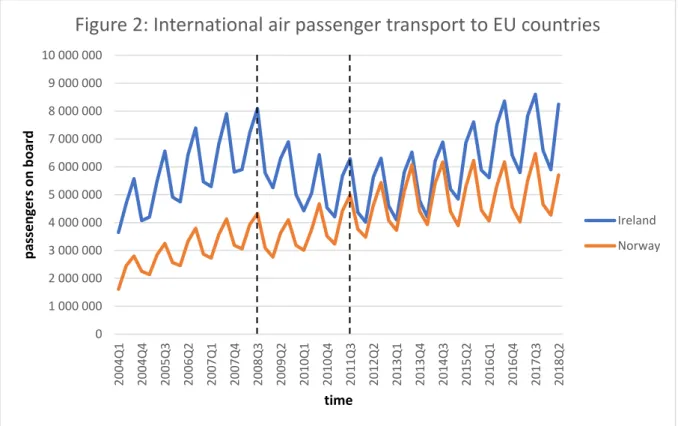
This section plots the trends for the dependent and independent variable in order to give a clearer understanding of the overall situation in the two chosen countries. The below figure depicts the trends for the dependant variable:

Dashed black lines indicate the highest and lowest years for traveller numbers in Ireland during the trimmed 2004-2011 sample

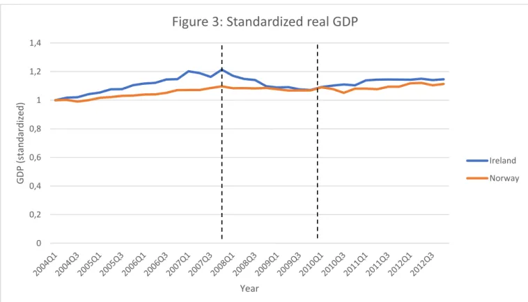
The triangular shapes in the above graph most likely displays the seasonal differences in passengers. In Ireland it is more common to holiday during the summer than in the winter, which might explain why the Irish slopes are steeper. In Norway winter activities like skiing are much more common and hence so too is the demand for winter travel. This is a possible explanation for why the Norwegian slopes are slightly flatter than the Irish ones. The above figure clearly demonstrates that up until 2008 the trends in both countries were remarkably similar. However, after 2008 the number of passengers in Ireland dropped considerably and continued to do so for a number of years, whereas in Norway the trends remained constant. With regards to the main explanatory variable we see a similar pattern. The figure below depicts the seasonally and calendar adjusted GDP expressed in terms of 2010 euros, in millions. In order to make comparisons between the two countries more straightforward, this chart was standardised where all values were divided by the value in year 1 for the two respective countries. 0 1 000 000 2 000 000 3 000 000 4 000 000 5 000 000 6 000 000 7 000 000 8 000 000 9 000 000 10 000 000 2004Q1 2004Q4 2005Q3 2006Q2 2007Q1 2007Q4 2008Q3 2009Q2 2010Q1 2010Q4 2011Q3 2012Q2 2013Q1 2013Q4 2014Q3 2015Q2 2016Q1 2016Q4 2017Q3 2018Q2 pass engers on boar d time

Figure 2: International air passenger transport to EU countries

Ireland Norway

(20)

12

Dashed black lines indicate GDP peak and trough for Ireland during the examined period

Again, similar to the trends in passenger numbers in Figure 2, the two countries GDP growth relatively tracks one and other up until 2008, at which point the Irish trend starts to fall. The downward effect here however recovers much quicker than it does in Figure 2, where GDP starts to increase again around the first quarter of 2010, whereas passenger numbers only pick up until around 2013. This could imply that there might be some sort of prolonged income effect which results in consumers cutting back on expenditure for an extended period, even after their relative incomes have recovered.

Finally, Table 1 below compares what happened to the number of international passengers both before and after the 2008 financial crisis in Norway and Ireland:

Table 1. Average number of international passengers, Difference-in-differences 2004-2011

Average number of international passengers per quarter

Pre period Post period Difference (post-pre) T = 1 5,563,832 5,714,732 150,900

T = 0 2,874,535 3,714,785 840,250 Difference in differences = 689,350

In this table (T=1) represents the treatment group, which is Ireland, and (T=0) is the control group, Norway. The passenger level of 2,874,535, for example, represents the average number

0 0,2 0,4 0,6 0,8 1 1,2 1,4 GDP (stand ardized) Year

Figure 3: Standardized real GDP

Ireland Norway

(21)

13

of international passengers per quarter in the control group during the pre-treatment period which runs from 2004Q1-2008Q1. The treatment period then commences from 2008Q1 until 2011Q4, where the average number of international passengers for the control group here is 3,714,785. By then taking the difference between these “pre” and “post” passenger numbers for the control group, I am able to calculate the average change in international passenger numbers per quarter for this group. The same is then done for the treatment group (T=1), and then these respective estimates are differenced across the treatment (T=1) and control (T=0) group in order to get the difference-in-differences estimate (DID). An average reduction of 689,350 passengers per quarter, represents the unconditional DID estimate. This means that as a result of being in Ireland after 2008Q1, there is a reduction in the number of passengers equal to this DID estimate. It is thus clear that after the financial crisis happened in 2008, the amount that the Irish people were flying significantly diminished.

6. Methodology

In order to estimate the income elasticity of demand for international air travel this study uses a DID/IV method. This involves using the 2008 financial crisis as an exogenous instrument for a change in income, in order to determine the unbiased relationship between income and international air passenger numbers. This method is appropriate to use in the case where the income variable is correlated with the error term, either as a result of being related to some omitted variable or if there is a situation of simultaneous causality where income and passenger numbers are both influencing each other. If either of these two situations exist, then estimating the income elasticity using standard OLS or fixed effects models will lead to biased estimates. Since the financial crisis however will be in no way impacted by passenger numbers and will also be unrelated to any omitted variables since it is an exogenous event, then using it as an instrument should allow to estimate the causality solely of income on passenger numbers. Using the financial crisis as an instrument thus allows to split up the income variable into two parts, one part correlated with the error term, and the other that is not. In the first stage of the model, the crisis is used to isolate the variation income, whilst being uncorrelated with the error term. This unbiased part of the change in income is then regressed on the number of international air passengers in the second stage of the model.

Before moving on to explaining the method used, it is first important to explain how the difference-in-differences was used in the context of this study. A difference-in-differences estimator calculates the average change in outcomes over time between a sample that is enrolled in a program (treatment group) and one that is not (control group). In other words, this difference-in-differences estimator gives the causal effect of being exposed to the treatment. For this paper the treatment would represent being subjected to the effects of the financial crisis of 2008. Now in order to determine this effect, what is needed is to find one country that was affected by the crisis and one that was not. If these two countries had similar pre-treatment trends, i.e. that the number of passengers travelling in both countries before the crisis hit in 2008 were parallel, as is the case for this study, then by prescribing the treatment to one country

(22)

14

and not the other, and then taking the difference, then this should give the effect of being exposed to the crisis. The assumption here is that if the country which was exposed to the crisis, had actually been relieved of these effects for some reason, then the number of passengers in this country would have continued to grow in line with the trends in the non-treated country, since the trends between the two were parallel before crisis hit.

When using this method, the treated country is Ireland and the non-treaded country is Norway. This is because Ireland was affected by the by the crisis of 2008 in a way in which Norway was not. Strict capital requirements, greater banking supervision and a general reluctance from Norwegian banks to invest in risky US sub-prime based bonds all contributed to the country’s stable economic performance throughout the period. As a result of this, the level of household spending in Norway was not negatively affected by the crisis so much as it was in Ireland. Regressing this difference-in-differences term on income should provide the effect that the financial crisis had on income in Ireland, thus providing the exogenous income change needed to estimate the unbiased income elasticity of demand for air travel.

7. Empirical strategy

This section starts by describing the reduced form specification of the model, followed by the DID/IV method. Furthermore, the main assumptions needed for unbiased estimates using this method are presented in section 7.3.

7.1. Reduced form estimation (baseline)

Before carrying out a DID/IV regression using the financial crisis as an instrument, the reduced form estimation of the model is first conducted in order to estimate the effect that the financial crisis in 2008 had on the number of international passengers in Ireland. This regression is set out as follows:

𝐿𝑜𝑔𝑃𝑎𝑠𝑠𝑎𝑛𝑔𝑒𝑟𝑠 _𝑖𝑡 = 𝛼₀+ 𝛼₁[𝑇𝑟𝑒𝑎𝑡𝑚𝑒𝑛𝑡]𝑡+ 𝛼2[𝑇𝑖𝑚𝑒]𝑖

+𝛼3[𝑇𝑟𝑒𝑎𝑡𝑚𝑒𝑛𝑡 ∗ 𝑇𝑖𝑚𝑒]𝑖𝑡+ 𝛼4𝑪𝒐𝒏𝒕𝒓𝒐𝒍𝒔𝑖𝑡+ 𝜀𝑖𝑡 (1)

The outcome variable in this above equation, “LogPassangers”, is the log number of international passengers. The “Treatment” term is a dummy equal to 1 if the country is Ireland and 0 if Norway, this captures possible differences between the two countries. “Time” is also a dummy term equal to 1 if after 2008 and 0 if before, this captures possible aggregate factors that would have an effect on the number of passengers even in the absence of the treatment. 𝛼₁

(23)

15

is the effect of being in Ireland and 𝛼₂ is the effect of being after 2008. The “Treatment * Time” interaction term is the same as a dummy variable equal to 1 if the observations are those both in the treated group after 2008. The 𝛼₃ coefficient thus, captures the effect of being in the treatment group after the treatment was implemented. It is the difference-in-differences estimate which essentially states the difference in changes between the two countries over time, or more simply, the effect that the financial crisis had on Ireland. 𝛼₀ represents the intercept which is the mean log number of passengers in the non-treated group before the treatment occurred, which would be Norway before the year 2008. Finally, “𝑪𝒐𝒏𝒕𝒓𝒐𝒍𝒔_𝑖𝑡” represents a vector of control variables including variables such as price.

Although the results generated from the reduced form are interesting to see, they do not directly provide the income elasticity of demand estimate, which is of course the main aim of this study. Instead this set up only captures the overall effect that the financial crisis had on the number of Irish passengers, which is shown by the 𝛼3 coefficient.

7.2. Difference-in-Differences Instrumental Variables model

This section describes the method used to estimate the income elasticity of demand for international air travel. I start by explaining the following equation which represents the first stage of the DID/IV method:

𝐼𝑛𝑐𝑜𝑚𝑒̂ 𝑖𝑡 = 𝛽0+ 𝛽1(𝑇𝑟𝑒𝑎𝑡𝑚𝑒𝑛𝑡)𝑡+ 𝛽2(𝑇𝑖𝑚𝑒)𝑖+ 𝛽3 (𝑇𝑟𝑒𝑎𝑡𝑚𝑒𝑛𝑡 ∗ 𝑇𝑖𝑚𝑒)𝑖𝑡 +

𝛽₄𝑪𝒐𝒏𝒕𝒓𝒐𝒍𝒔_𝑖𝑡+ 𝜖_𝑖𝑡 (2)

The outcome variable “𝐼𝑛𝑐𝑜𝑚𝑒̂ _𝑖𝑡” , represents the log of income, “𝑇𝑟𝑒𝑎𝑡𝑚𝑒𝑛𝑡_𝑡” and “𝑇𝑖𝑚𝑒_𝑖” are the country and time fixed effects. “𝑇𝑟𝑒𝑎𝑡𝑚𝑒𝑛𝑡_𝑡”, as it was previously, is a treatment group dummy equal to 1 if the country belongs to the treated group, which is Ireland, and 0 if it is the non-treated group, Norway. “𝑇𝑖𝑚𝑒_𝑖” is again the treatment time dummy which is equal to 1 for observations after the financial crisis began, which this paper defines as 2008 onwards, and 0 for observations before the crisis hit i.e. before 2008. 𝛽₁ represents the effect of being in the treatment group and 𝛽2 is the effect of being in the post treatment group. “𝑪𝒐𝒏𝒕𝒓𝒐𝒍𝒔𝒊𝒕”

represents a vector of control variables. With regards to the control variables selected it is important that these are in no way influenced by the treatment itself. This is a required assumption when using an instrumented difference-in-differences design. The aim is to capture the effect that the financial crisis had solely on the income variable, therefore if I include other variables which were affected then this will impede the estimation of the crisis’ real effect on income. For this reason, potential controls such as unemployment and government expenditures, which both arguably will influence the number of passengers travelling, were ruled out of this model. The 𝛽3 coefficient, which multiplies with the interaction term,

(24)

16

income of living in Ireland after the 2008 financial crisis occurred, for which in this case the interaction term would be equal to 1. Estimating equation (2) is of considerable intrinsic interest because it estimates the impact that the financial crisis had on Irish people’s income. Of course, this is under the assumption that the “treated” group, Ireland, was affected by the crisis, whereas the “non-treated” Norway, was not. This is an issue which will be addressed in more detail in the next section. This first stage equation above will determine if the first condition for a valid instrument, which states that the instrument must have an effect on the main explanatory variable, is fulfilled.

The second stage of the model involves regressing the log number of passengers on the newly generated income variable found from the first stage. As a result of using the instrument in the first stage, this newly generated income variable should now be unrelated to the error term. The below equation is used to estimate the causal effect of income on the number of passengers:

𝐿𝑜𝑔𝑃𝑎𝑠𝑠𝑎𝑛𝑔𝑒𝑟𝑠_𝑖𝑡 = 𝛾₀ + 𝛾₁(𝑇𝑟𝑒𝑎𝑡𝑚𝑒𝑛𝑡)_𝑡+ 𝛾₂(𝑇𝑖𝑚𝑒)_𝑖+ 𝛾₃(𝐼𝑛𝑐𝑜𝑚𝑒̂ _𝑖𝑡) + 𝛾₄𝑪𝒐𝒏𝒕𝒓𝒐𝒍𝒔_𝑖𝑡+ 𝜀_𝑖𝑡 (3)

Here “𝑇𝑟𝑒𝑎𝑡𝑚𝑒𝑛𝑡_𝑡” and “𝑇𝑖𝑚𝑒_𝑖” again represent the time and country fixed effects. “𝑪𝒐𝒏𝒕𝒓𝒐𝒍𝒔_𝒊𝒕” is again a vector of control variables as it was in equation (2).

“𝐿𝑜𝑔𝑃𝑎𝑠𝑠𝑎𝑛𝑔𝑒𝑟𝑠𝑖𝑡” is the log number of international air travellers within the 28 EU

countries. “𝐼𝑛𝑐𝑜𝑚𝑒̂ _𝑖𝑡” is the log projected income variable that was generated from the first stage regression. Finally, 𝛾₃, is the coefficient of interest, which is the income elasticity estimate. The fact that I use the log values of income and air passengers instead of the total values is done so that I can directly retrieve the elasticity estimates without having to manipulate the results. This allows to transform highly skewed variables into more symmetric ones (Carmona-Benítez et al. 2017). Therefore, the estimated 𝛾₃ coefficient can be directly interpreted as the income elasticity of demand for international air travel, where it expresses the percentage change in the demand for air travel as a result of a one percent change in income.

7.3. Required assumptions for identification

Before moving onto the results section, it is first important to highlight the important assumptions that should be fulfilled in order for the findings of this study to be valid. Since this study is using a DID/IV method, it is then subject to the requirements of both difference-in-differences and instrumental variable methods. This section outlines these requirements and discusses potential issues with identification.

When carrying out a difference-in-differences experiment there are a number of key assumptions that should be fulfilled. The most important of these however is the parallel trend, or common trend, assumption. This assumption states that the pre-treatment trends for the

(25)

17

control and treatment groups are parallel up until the treatment. In other words, it requires that in the absence of the treatment, the difference in outcomes between the two groups will be constant over time. This would imply that if the treated group had not received the treatment, then the trends for this group would have continued the same as those for the control group. The best way to see whether this condition is fulfilled is to plot the trends between the two groups graphically, as was done in Figure 2 in section 5. This figure clearly showed that up until the treatment began in 2008, the trends in the number of passengers between Ireland and Norway were parallel. However, this graph only depicts the unconditional trends, whereby it does not control for additional factors that affect demand. These additional factors could include issues such as differences in passenger numbers depending on the season, certain country fixed effects, or changes in air fares, all of which will have an impact on the number of passengers. In order to be sure that the trends are truly parallel, this paper will plot the residual trends in section 9, which will show the conditional trends after these additional factors have been controlled for.

The second key assumption for a difference-in-differences method is known as the Stable Unit Treatment Value assumption. This implies that one, and only one, of the potential outcomes are observable for each group and that there should be no spill over effects of the treatment on the control group (Lechner, 2011). This could be a potential issue for this study since there is a possibility that the control group, Norway, may have also been affected by the financial crisis. If this were to be the case, then it would not be possible to estimate the precise value of the causal effect. If Norway was indeed negatively affected by the financial crisis then this would mean that the results of this paper would be biased downwards, where the income effect is underestimated. Another important implication of the SUTVA is that there are no relevant interactions between the control group and the treatment group, and thus the composition of the two groups is stable over time. This could be another potential issue for this paper in the case where people might have moved from one country to the other during the time period of this study.

When selecting an instrument using an instrumental variables (IV) method there are two key conditions which must be fulfilled in order for the instrument to be valid. The first condition is known as instrumental relevance which states that the instrument must be correlated with the main explanatory variable, which in this case is income. If we have a condition where there is a significant correlation between the chosen instrument and the main explanatory variable, then this is known as a strong first stage. This relationship will be provided when carrying out the first stage regression of the model. The second condition for a valid instrument is instrumental exogeneity which implies that the chosen instrument cannot be correlated with the error term. This condition also implies that the instrument should only be correlated with the dependent variable through its effect on the explanatory term. Thus, in order for the financial crisis to be a good instrument it should be correlated with income, it should not be related to any omitted variables in the model which also affect the number of travellers, and it should have no direct effect on the number of air travellers except through a change in income. With regards to instrumental relevance, it seems highly likely that the crisis had an adverse effect on people’s relative income, due largely to the increased unemployment, reduced expenditure, and reduced output that it caused throughout most of Europe and the US at the time of its occurrence.

(26)

18

Furthermore, since the crisis was an exogenous event which surprised people, then this would mean that it should be unrelated to any of the endogenous variables contained within a standard OLS model regressing income on the number of air travellers. Additionally, since this paper is capturing the effect of the financial crisis using a DID approach, then this would make the instrument exogenous so long as the DID assumptions hold.

An area of concern however relates to the assumption that the instrument only affects the dependent variable through the main explanatory one. This means that the financial crisis should only impact the number of air passengers through its effect on people’s income. Although this seems like a relatively plausible idea, there is the potential for a situation to emerge whereby the crisis reduces the amount that people fly through fear over future job prospects or negative expectations about future earnings. This issue however will be addressed more thoroughly in the discussions section.

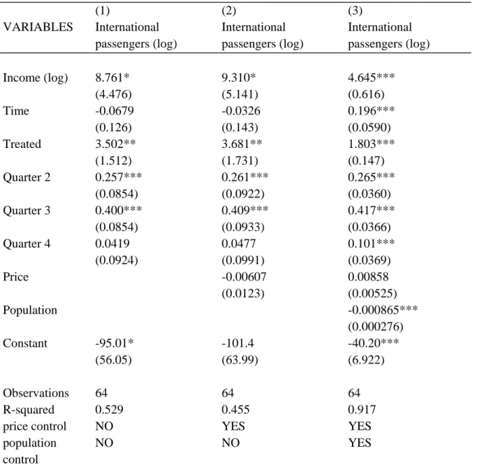
8. Results

This section presents the key results from this study. First of all, the baseline results estimated using the reduced form specification are covered. Afterwards the first and second stage results from the DID/IV method are displayed, where the income elasticity of demand for air travel was found.

8.1. Reduced form estimates

Table 2 below provides the basic reduced form estimates regressing the number of international air passengers on the difference-in-differences coefficient, which captures the effect of the financial crisis on Ireland.

(27)

19

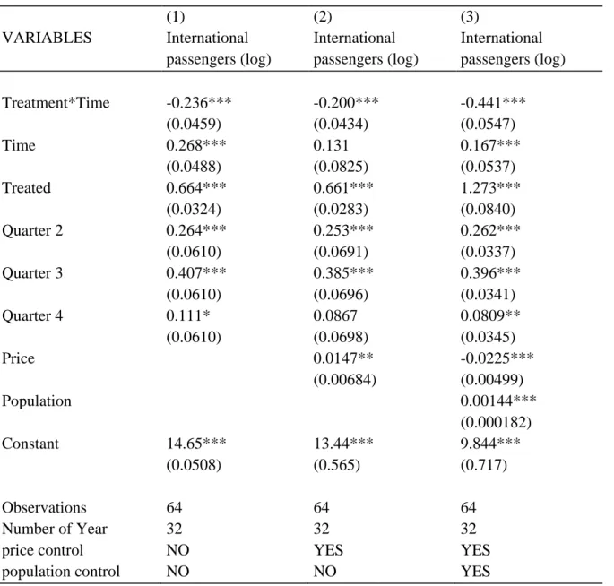
Table 2: Baseline Estimates

Standard errors in parentheses *** p<0.01, ** p<0.05, * p<0.1

The estimated coefficient for the “Treatment*Time” interaction term in column 1 shows a 23.6% reduction in the number of travellers in Ireland after the 2008 financial crisis started. This estimate does not include price or population control. When these two variables are included, as seen in column 3, then the effect increases to 44%. This clearly demonstrates that the financial crisis had a significant negative impact on international passenger numbers in Ireland. There are of course numerous factors which could have also influenced this result. This paper attempts to control for the most obvious of these. Quarterly controls are included which represent dummy terms for each quarter, where quarter 1 is omitted to avoid multicollinearity. Referring to column 1, there is 26.4% more passengers flying in quarter 2 than there is in quarter 1. Quarter 3 is the most popular month to travel where there are more than 40% more passengers flying. Lastly for quarter 4 there is roughly 11% more passengers flying than during quarter 1. These findings are in line with what would be expected in reality,

(1) (2) (3) VARIABLES International passengers (log) International passengers (log) International passengers (log) Treatment*Time -0.236*** -0.200*** -0.441*** (0.0459) (0.0434) (0.0547) Time 0.268*** 0.131 0.167*** (0.0488) (0.0825) (0.0537) Treated 0.664*** 0.661*** 1.273*** (0.0324) (0.0283) (0.0840) Quarter 2 0.264*** 0.253*** 0.262*** (0.0610) (0.0691) (0.0337) Quarter 3 0.407*** 0.385*** 0.396*** (0.0610) (0.0696) (0.0341) Quarter 4 0.111* 0.0867 0.0809** (0.0610) (0.0698) (0.0345) Price 0.0147** -0.0225*** (0.00684) (0.00499) Population 0.00144*** (0.000182) Constant 14.65*** 13.44*** 9.844*** (0.0508) (0.565) (0.717) Observations 64 64 64 Number of Year 32 32 32

price control NO YES YES

(28)

20

where people generally tend to fly more during the summer months than they do during the winter. With regards to price and population these do not have much of an effect on passenger numbers. In previous literature price is usually found to be one of the key determinants of air travel numbers, therefore it is a little surprising that the results of this study find no effect. This could be down to that fact that I use a packaged holiday variable to represent price instead of specific airline flights. The “Treated” term in the above table shows a very large positive value which is because the number of international passengers in Ireland per quarter is much higher than for Norway. Finally, “Time” has a small positive value which implies that the number of passengers is slightly increasing over time.

8.2. DID/IV estimates

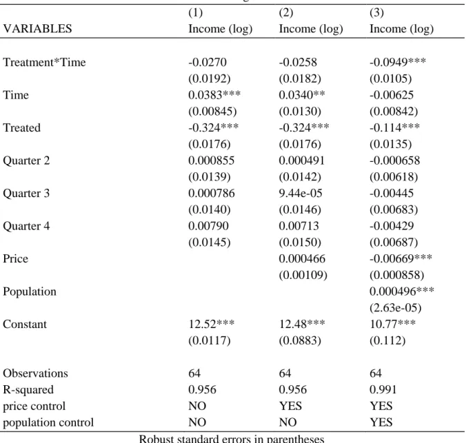
This section provides the main results from this study using the DID/IV method. Table 3 first presents the results from the first stage of the model where the difference-in-differences term, capturing the effect the crisis had in Ireland, was regressed on the income variable. The relationship between these two variables was estimated to be between -2.7% and -9.49% which would imply that the crisis did have a negative effect on income. This would confirm that the second requirement for a valid instrument, whereby the instrument is related to the main explanatory variable, is fulfilled.

(29)

21

Table 3: First stage estimates

(1) (2) (3)

VARIABLES Income (log) Income (log) Income (log) Treatment*Time -0.0270 -0.0258 -0.0949*** (0.0192) (0.0182) (0.0105) Time 0.0383*** 0.0340** -0.00625 (0.00845) (0.0130) (0.00842) Treated -0.324*** -0.324*** -0.114*** (0.0176) (0.0176) (0.0135) Quarter 2 0.000855 0.000491 -0.000658 (0.0139) (0.0142) (0.00618) Quarter 3 0.000786 9.44e-05 -0.00445 (0.0140) (0.0146) (0.00683) Quarter 4 0.00790 0.00713 -0.00429 (0.0145) (0.0150) (0.00687) Price 0.000466 -0.00669*** (0.00109) (0.000858) Population 0.000496*** (2.63e-05) Constant 12.52*** 12.48*** 10.77*** (0.0117) (0.0883) (0.112) Observations 64 64 64 R-squared 0.956 0.956 0.991

population control NO NO YES

Robust standard errors in parentheses *** p<0.01, ** p<0.05, * p<0.1

Table 4 below presents the main results from the second stage of the model where I regressed the exogenous income variable generated from the first stage on international passenger numbers. Panel (1) presents the results without price or population controls. The income elasticity of demand estimate here is 8.761, which means that an increase in income of 1% will lead to an 8.761% increase in the demand for international air travel. This result implies that the demand for air travel is highly elastic with regards to a change in income. According to this finding, air travel would be defined as a luxury good.

(30)

22

Table 4: Second stage estimates

(1) (2) (3) VARIABLES International passengers (log) International passengers (log) International passengers (log) Income (log) 8.761* 9.310* 4.645*** (4.476) (5.141) (0.616) Time -0.0679 -0.0326 0.196*** (0.126) (0.143) (0.0590) Treated 3.502** 3.681** 1.803*** (1.512) (1.731) (0.147) Quarter 2 0.257*** 0.261*** 0.265*** (0.0854) (0.0922) (0.0360) Quarter 3 0.400*** 0.409*** 0.417*** (0.0854) (0.0933) (0.0366) Quarter 4 0.0419 0.0477 0.101*** (0.0924) (0.0991) (0.0369) Price -0.00607 0.00858 (0.0123) (0.00525) Population -0.000865*** (0.000276) Constant -95.01* -101.4 -40.20*** (56.05) (63.99) (6.922) Observations 64 64 64 R-squared 0.529 0.455 0.917

population control

NO NO YES

Standard errors in parentheses *** p<0.01, ** p<0.05, * p<0.1

Similarly to the reduced form estimates in table 2, the quarterly controls suggest that there is a positive effect on the number of passengers from flying in the second and third quarter. In panel (2), I now include a price control. This control has little effect on the number of passengers, however after including it the income elasticity estimate increases slightly to 9.310. Everything else in this panel remains largely unchanged. The income elasticity in the first two panels are statistically significant at the 5% level. Finally, in panel (3) I add a population control in addition to controlling for price. This results in a somewhat lower estimate of 4.645, which is now statistically significant at the 1% level. These findings imply that consumers demand for air travel is highly elastic to a change in income.

(31)

23

9. Robustness checks

This section carries out several robustness checks to see how stable the results are, as well as to check their validity. First of all, a residual plot is done in order to test whether the trends are truly parallel, conditional on the control variables. Next a leads and lags test to examine the effect in individual quarters is completed. This will allow to investigate if there were any pre-treatment effects, and also determine which post pre-treatment quarters saw the biggest decrease in passenger numbers. Lastly, different definitions of the crisis are tested to see how much this impacts the estimates.

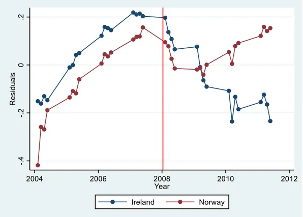
9.1. Residual plot

The first robustness test is a residual plot where I aim to show the conditional trends in the number of air travellers in both countries after controlling for the variation caused by the control variables. This is done by estimating the residuals from the following model:

𝐿𝑜𝑔𝑃𝑎𝑠𝑠𝑎𝑛𝑔𝑒𝑟𝑠𝑖𝑡 = 𝛾0+ 𝛾1(𝑇𝑟𝑒𝑎𝑡𝑚𝑒𝑛𝑡)𝑡+ 𝛾2(𝑇𝑖𝑚𝑒)𝑖+ 𝛾3𝑪𝒐𝒏𝒕𝒐𝒓𝒍𝒔𝑖𝑡 + 𝜀𝑖𝑡

(4)

Here I regress the number of air travellers on everything excluding the difference-in-differences term, which captures the effect of the treatment. The residuals from this regression are plotted in Figure 4 below. These are the difference between the observed value of the dependent variable and the predicted value (Bruce and Bruce, 2019). If this model explains the relationship between the variables of interest well, then it should be the case that the residuals will be close or equal to zero. This should mean that the only variation left in the passenger trends is from the treatment itself.

(32)

24

Figure 4: Residual plot graphing the conditional trends in international air passenger numbers

Red line indicates the beginning of the financial crisis in 2008

What this figure shows is the trends in the number of passengers after controlling for everything except the effect of the financial crisis. It is clear that the pre-treatment trends for both countries, after controlling for the control variables, are indeed parallel. This is evidence that the parallel trends assumption is truly satisfied. When looking at the trends after 2008 it is apparent that the number of passengers in Ireland drops significantly and continues to do so until at least 2012. However, referring to the Norwegian plots, it is evident that there is also a drop for this country too. This would imply that the control group for this study was also affected by the treatment, which would be a sure violation of the SUTVA assumption. Although the trends begin to pick up again relatively quickly in 2009, it is still an issue with regards to the validity of this study. After 2009, the Norwegian trends pick back up whereas the Irish ones continue to fall. This is the period which is most likely driving the results presented in table 4.

9.2. Experimenting with crisis year definition

In this section I examine the effect on the results after modifying the dates that I define as “crisis years”. The main issue here relates more to defining the end date of the crisis rather than the starting one, which is widely agreed upon, therefore I only change the former. Table 5 below depicts the results after carrying out such changes:

(33)

25

Table 5: Experimenting with different “crisis” years

(1) (2) (3) (4)

VARIABLES crisis ends 2012 crisis ends 2011 crisis ends 2010 crisis ends 2009 Income 10.28** 8.761* 5.194*** 2.544** (4.855) (4.476) (1.967) (1.224) Quarter 2 0.257*** 0.257*** 0.253*** 0.269*** (0.0968) (0.0854) (0.0447) (0.0251) Quarter 3 0.413*** 0.400*** 0.407*** 0.402*** (0.0966) (0.0854) (0.0446) (0.0251) Quarter 4 0.0436 0.0419 0.0730 0.0947*** (0.102) (0.0924) (0.0472) (0.0273) Treated 3.994** 3.502** 2.346*** 1.488*** (1.651) (1.512) (0.665) (0.410) Time -0.158 -0.0679 0.0477 0.121*** (0.164) (0.126) (0.0501) (0.0321) Constant -114.0* -95.01* -50.37** -17.19 (60.81) (56.05) (24.63) (15.33) Observations 72 64 56 48 R-squared 0.269 0.529 0.897 0.975

Although the results all remain positive, the magnitude of this positivity differs significantly depending which end date is chosen. It is evident that the longer the time period I define as the crisis, the larger the income elasticity estimate. This could potentially be because a financial crisis is an event which usually has long lasting effects even after the initial crisis is over. Additionally, since Figure 4 shows that Norway was also affected in 2008 and 2009, then if I assume that the crisis ended in 2009, the results are much smaller. Given that the Norwegian trends picked up again after 2009 and continued to rise, whereas the Irish ones continued to fall, it makes sense that the longer I define the financial crisis to have the lasted, the larger the results will become.

9.3. Leads and lags test

The next robustness check that was done was a leads and lags test to examine the effects in each individual quarter. This involved creating dummy variables for each quarter and regressing these on the log number of international passengers. This allowed to determine if there was any pre financial crisis effects, as well as to check which post crisis quarters had the largest effect and were thus driving the results. The test should also allow to identify whether there was some kind of delayed expenditure effect where people were still cutting back on

(34)

26

flying even after the crisis had ended, and their relative incomes had recovered. Using the full set ranging from 2004-2018 garners the following results:

Table 6: Leads and Lags test (1)

VARIABLES International passengers (log) All quarters after 2011 Q1 -0.259**

(0.0995) 2010 Q4 -0.312*** (0.0958) 2010 Q3 -0.292*** (0.0945) 2010 Q2 -0.378*** (0.0957) 2010 Q1 -0.303*** (0.0790) 2009 Q4 -0.287*** (0.0950) 2009 Q3 -0.286*** (0.107) 2009 Q2 -0.219** (0.103) 2009 Q1 -0.169 (0.118) 2008 Q4 -0.139 (0.126) 2008 Q3 -0.0897 (0.131) 2008 Q2 -0.0314 (0.112) 2007 Q4 0 (omitted) 2007 Q3 -0.00941 (0.103) 2007 Q2 -0.0186 (0.103) 2007 Q1 -0.0379 (0.113) 2006 Q4 -0.0682 (0.0954) 2006 Q3 -0.0614 (0.120) 2006 Q2 -0.0540 (0.124) All quarters before 2006 Q1 -0.271***

(0.0755)

Observations 116

R-squared 0.859

Robust standard errors in parentheses *** p<0.01, ** p<0.05, * p<0.1

This table also included country, time, price and seasonal controls, which were hidden due to space limitations. The full results table for this regression along with the equation describing the set-up of the model can be found