Hybrid Energy System for Off – Grid Rural Electrification(Case study Kenya)

(1)

0 MSC WIND POWER PROJECT MANAGEMENT, GOTLAND UNIVERSITY

Hybrid Energy System for Off –

Grid Rural Electrification

(Case study Kenya)

Department of Wind Energy Gotland University

Author: Clint Arthur Ouma

Supervisor: Dr. Bahri Uzunoglu Examiner: Prof. Jens Sorensen

5/30/2011

(2)

1

List of Figures and Tables

FIGURE 1:MAP OF THE NATIONAL ELECTRIC GRID SYSTEM IN KENYA [5] ...5

FIGURE 2:MAP OF INSTALLED WIND PUMPS,WIND TURBINES AND SMALL WIND GENERATORS IN KENYA [5] ...8

TABLE 1:AVERAGE MONTHLY WIND SPEEDS FOR 12SITES IN KENYA AT 10M HEIGHT IN KNOTS... 11

FIGURE 3:GRAPHS OF WIND SPEED IN KNOTS... 12

FIGURE 4:TOP THREE SITES MEASURED IN KNOTS ... 12

FIGURE 5:MAP OF KENYA WITH ANNUAL AVERAGE WIND SPEEDS AT THE 12SAMPLE LOCATIONS IN KNOTS ... 14

TABLE 2:MARSABIT DATA PROPERTIES IN WINDORGRAPHER ... 15

TABLE 3:DATA SUMMARY FOR MARSABIT IN WINDORGRAPHER ... 16

FIGURE 6:MARSABIT DIURNAL CYCLE BY MONTH –WINDORGRAPHER INTERFACE ... 16

FIGURE 7:MEAN DIURNAL WIND PROFILE BY MONTH AS EVALUATED IN WINDOGRAPHER –PRESENTED IN EXCEL ... 17

FIGURE 8:MONTHLY DURATION CURVE FOR MARSABIT EXPORTED TO MICROSOFT EXCEL FROM WINDOGRAPHER .... 17

TABLE 4:VOI DATA PROPERTIES IN WINDORGRAPHER ... 18

TABLE 5:DATA SUMMARY FOR VOI IN WINDORGRAPHER ... 18

FIGURE 9:VOI DIURNAL CYCLE BY MONTH –WINDOGRAPHER INTERFACE ... 19

FIGURE 10:VOI DIURNAL WIND PROFILE BY MONTH AS EVALUATED IN WINDOGRAPHER ... 20

FIGURE 11:MONTHLY DURATION CURVE FOR VOI EXPORTED TO MICROSOFT EXCEL FROM WINDORGRAPHER ... 20

FIGURE 12:TIME SERIES BY MONTHLY MEAN WIND SPEEDS OVER SIX YEARS FOR VOI ... 21

FIGURE 13:WIND SHEAR PROFILE FROM WINDPRO AND WASP ... 22

FIGURE 14:VOI SATELLITE IMAGE ... 24

FIGURE 15:MAP OF VOI REGION SHOWING TSAVO NATIONAL PARK ... 24

TABLE 6:ELECTRICITY CONSUMPTION FOR TYPICAL NAIROBI HOUSEHOLD IN (KWH) ... 27

FIGURE 16:AVERAGE ANNUAL HOUSEHOLD ELECTRICITY CONSUMPTION BY SECTOR IN KENYA [5]... 28

TABLE 7:PROJECTED PRIMARY ELECTRICITY LOAD ... 31

TABLE 8:PROJECTED DEFERRABLE ELECTRICITY LOAD... 33

FIGURE 17:PRIMARY LOAD INPUT DATA IN HOMERSOFTWARE ... 36

FIGURE 18:SECONDARY LOAD INPUT DATA IN HOMERINTERFACE ... 37

FIGURE 19:EQUIPMENT TO CONSIDER IN THE HYBRID SETUP ... 37

(4)

3

TABLE 8:COST ESTIMATES FOR WIND TURBINES ... 39

FIGURE 21:GENERIC 20KWWIND TURBINE INPUT VALUES ... 39

FIGURE 22:FUHRLÄNDER WIND TURBINE INPUT DATA ... 40

FIGURE 23:BATTERY INPUT DATA ... 41

FIGURE 24:CONVERTER INPUT DATA ... 42

FIGURE 25:WIND RESOURCE INPUT DATA ... 43

FIGURE 26:WIND SPEED VARIATION WITH HEIGHT;POWER LAW PROFILE ... 44

FIGURE 27:WIND SPEED VARIATION WITH HEIGHT;LOGARITHMIC PROFILE ... 44

FIGURE 28:FUEL RESOURCE INPUT DATA ... 45

FIGURE 29:PRICE RANGE OF DIESEL $/L ... 45

FIGURE 30:SYSTEM CONTROL INPUT DATA ... 47

FIGURE 31:FEED IN TARIFF FRAMEWORK IN KENYA [1]... 47

TABLE 9:UPPER COST LIMIT RESULTS FROM SIMULATIONS OF FUHRLÄNDER 30KWTURBINES AT 25,30 AND 40M HUB HEIGHTS ... 50

FIGURE 32:COMPARISON OF NUMBER OF TURBINES AND GENERATOR CAPACITY IN RELATION TO HUB HEIGHT AND DIESEL PRICE ... 51

FIGURE 33:COMPARISON OF GENERATOR AND WIND POWER PRODUCTION IN RELATION TO HUB HEIGHT AND DIESEL PRICE ... 51

TABLE 10:LOWER COST LIMIT RESULTS FROM SIMULATIONS OF FUHRLÄNDER 30KWTURBINES AT 25,30 AND 40M HUB HEIGHTS ... 52

FIGURE 34:COMPARISON OF NUMBER OF TURBINES AND GENERATOR CAPACITY IN RELATION TO HUB HEIGHT AND DIESEL PRICE ... 53

FIGURE 35:COMPARISON OF GENERATOR AND WIND POWER PRODUCTION IN RELATION TO HUB HEIGHT AND DIESEL PRICE ... 53

(5)

4

Hybrid Energy System for off – grid

rural electrification (Case study Kenya)

Abstract

The aim of this thesis study is to design a hybrid energy system comprised of wind turbines, diesel generators and batteries to provide electricity for an off - grid rural community in Kenya. Wind Measurements collected over six years from 12 locations in Kenya have been studied and one site selected for this project due to its wind potential, geographical location and socio-economic potential. The energy system is designed to cater for the electricity demand of 500 households, one school, one medical clinic and an irrigation system. The system will support up to 3000 people. The Hybrid Optimization Model for Electric Renewables (HOMER) is the software tool that has been used to simulate the hybrid system and analyze its results. The optimization has been carried out and presented according to cost of electricity and sensitivity graphs have been used demonstrate the optimization based on diesel price and wind turbine hub height.

Key words

Hybrid Energy System, Wind Power, Hybrid Power Optimization, Off–Grid Rural Electrification

(6)

5

Introduction

The access to electricity has proven to be a key factor necessary for socioeconomic development, both for the peoples and infrastructure of a region. It is a cornerstone for urbanization and industrialization in these modern times. With electricity lines being confined to large cities and along major transport lines, developing countries lag far behind in many sectors when compared to industrialized countries. Kenya, despite being the leader in development in the Eastern African region, has a very poor electricity penetration rate. Electricity is available for only 15% of the population and caters for only 9% of the country’s primary energy consumption [1].

Figure 1: Map of the National Electric Grid system in Kenya [5]

This thesis aims at addressing the electricity penetration problem from a bottom-up approach by the implementation of a wind, diesel generator and battery powered hybrid system. We realize that, regions with attractive wind resources and no access to the national grid are able to generate their own electricity. Secondly, it is more attractive for the electric grid to be extended to a point of electricity production rather than consumption. This

(7)

6 project’s primary aim is to design a system that will run independent of the national grid, in a region that does not have electricity access. The secondary aim is to provide a rural community with a system that is both socially and economically beneficial to the residents as well as environmentally friendly thus taking the three pronged approach that encompass the pillars of sustainable development; economical, social and environmental [4]. According to the population census carried out in 2009 for Kenya, 67.7 % of the country’s 38,610,097 citizens live in the rural areas [13] any successful efforts to improve productivity in these regions would have a significant impact on national growth.

The project is set to meet the needs of a small community comprised of 500 households. This project uses assumptions based on a study carried out in Ethiopia for a Wind-Solar-Diesel hybrid system by Getachew Bekele and Björn Palm in March 2009 at KTH University, Stockholm [11]. It consists of a renewable electricity generation system designed to run 500 homes, a school, a local clinic and an irrigation system to help the people engage in agricultural activities. The concept is to provide enough power to run a system that will allow the residents to generate income and food security independently. The total population to be serviced by this project is to be about 3000 people; that is 500 families of five members each (two parents and three children) and five hundred additional people [11].

(8)

7

1. Background

Due to unreliable supply and the absence of electricity in several parts of the country, many individual home owners have taken on the burden of meeting their own energy needs which are in most cases unsustainable and in some cases, very expensive. Entrepreneurs are leading the way with several small and medium sized companies supplying home solar power systems. There are reports that by 2006, up to 100 000 were using solar ovens for cooking [2] and about 50 000 solar water heating systems were produced and sold between 1981 and 2002 [5] but due to the expense incurred, only 2% of rural inhabitants use the technology [2]. Solar PV units, though productive, have been avoided in recent years because there have been cases of theft involving the panels [12]. The reliance on firewood for cooking coupled with clearance of forests for agricultural purposes led to large scale deforestation that led to the depletion of the country’s forest cover from 10% in the 1960’s to 1.7% in the year 2006 according United Nations reports [6]. Efforts are indeed underway to increase electricity penetration in the country with the governmental organizations setting ground breaking policies to encourage investment but grid extension remains a major obstacle as is the case in Europe.

The use of wind power for electricity generation in Kenya has only begun gaining momentum in recent years. Initially exploitation of wind power for energy generation was done on individual basis by Independent power producers (IPPs) this could possibly be due to the risks involved in the business. In this stance the main technology in use was wind pumps and few battery chargers as is reflected in the UN Energy Atlas for Kenya [5]. Figure 2 shows a map of Kenya that highlights the locations of installed wind pumps, wind turbines and small wind generators in the country by 2005 [5].

(9)

8 Figure 2: Map of Installed Wind Pumps, Wind Turbines and Small Wind Generators in Kenya [5]

The use of wind power for electricity generation was first introduced in the country in 1984 when the first wind turbines for electricity generation in Kenya were installed in Ngong’ hills and Marsabit for 400 kW and 200 kW respectively through a grant issued by the Belgian government. Today, Kenya’s first wind farm stands at Ngong’ hills pumping 5.1 MW of electricity into the national grid while construction of Africa’s largest wind farm (300 MW) is underway at Marsabit and is expected to go online between June 2011 and July 2012 [1]. Now, wind power is very attractive in the country and has gained a lot of governmental support with a feed in tariff system [1] coming into play making wind power the cheapest source of electricity in the country. Kenya does not have natural gas or oil reserves and uses hydro power plants to generate up to 64% of its electricity [3]. Recent droughts and rise in oil prices have caused the governmental bodies to revive their interest in renewable energy sources such as wind power and geothermal energy [5].

(10)

9 The location of Kenya on the planet, with the equator virtually cutting the country in half, leads people to believe that solar energy is the most viable resource for exploitation. It is true that Kenya has high solar irradiation levels throughout the year and the vast savannah grasslands and wide open spaces would be conducive for such technologies. Nevertheless, solar energy technology remains about 3.5 times more expensive than wind energy [7] this raises the prospects of using wind power for large scale electricity production in accordance with the Least Cost Power Development Plan (LCPDP) for Kenya [8].

It is typical that wind speeds accelerate towards higher latitudes and are generally low around the equator which is due to the Hadley cell phenomena where the atmosphere above the equator are characterised by vertical winds that make a cycle out towards the poles. Kenya has some naturally occurring advantages that allow it to have strong high speeds in certain regions. The winds in the northern part of the country are mostly influenced by physical geographical features such as the Great Rift Valley, Lake Turkana and certain mountains, hills and ridges that cause a channelling effect thus accelerating wind speeds in the more arid regions of the country [9].

Southern regions of the country and especially in the coast province are directly affected by the monsoon winds that blow over the Indian Ocean. The regular flowing winds that carried traders north and south along the East African coast from Saudi Arabia and India to Southern Africa have remained consistent through the ages and are now being looked upon as the next energy source to usher in a new way of life for the residents of the African coast. These winds dictate the trends for most regions in Kenya that exhibit good to excellent wind resources which peak when the southerly monsoons or locally known as ‘Kusi’ blow between April and mid-September [10], [14]. The North Easterly Monsoon Trade winds blow from December to mid – March and are locally known as ‘Kaskazi’ these winds are famous for faring traders southwards. The transitional period in March is short lived and usually goes unnoticed lasting only a few weeks but the period from September to November is known as ‘Matalai’ and holds much significance as it brings rains to the coastal regions *10+.

(11)

10

2. Wind Potential in Kenya

The generation of electricity from wind energy is mainly dependent on the wind regime in the region of interest. This makes the science site specific; as such, reliable long term wind measurements (at least one year) need to be studied before making a decision on where to locate your wind farm. The models used for remote wind data analysis can be grouped as diagnostic and prognostic models [17].

The diagnostic or analytical models such as WASP, WindPRO and Wind Farmer are most commonly used for preliminary wind data assessment. These are simple to use and easy to interpret. Prognostic models have a higher complexity than diagnostic ones. They require more powerful computers to run simulations and take much more time to obtain results. They include models that use Complex Fluid Dynamics (CFD) such as WindSim for computations and Meso scale models such as MIUU and MASS [17].

2.1. Wind Data Analysis

In this thesis, measurements from meteorological weather stations have been used to map out the wind characteristics and gauge the amount of electricity that a wind power system can generate in the most interesting site. The reliability of wind statistics increases with the length of the period of collection as long term data makes prediction of future trends more accurate. In this case, the data in use has been provided from twelve meteorological weather stations from different locations in Kenya and covers the six year period between January 1995 and December 2000; measurements have been taken for every hour of everyday at 10 meters above the ground in knots [15]. Other sources of wind data such as NCEP, MERRA and NCAR were not readily accessible and the meteorological station records were sufficient to run a preliminary study such as this thesis work.

Some of the locations have measurements of less than one year and thus will not be used in the final comparison. Tables and graphs have been made to represent the results of the monthly wind profiles in these twelve locations. Four locations have recordings of less than one year while the rest have six years´ data. The best locations for the project, according to wind power potential will be highlighted in the final graph. Other criteria in site selection such as the geographical location, the distance of the site from the existing grid, the lifestyle of the residents and the availability of water, will be applied in the ensuing chapters of this document. Once a site has been decided on for this project, the measured data will be used in WindPRO/ WAsP in simulations to determine wind speed at different heights to allow us optimize the system for different hub heights. The measurements were taken for the following sites;  Eastleigh  Lodwar  Machakos  Marsabit  Msabaha  Mtwapa  Mandera

 Nairobi Airport (Embakasi)

 Thika

 Voi

 Wajir

(12)

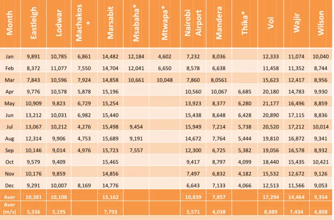
11 Table 1 and the graphs in figures 3 and 4 below show the results obtained from the averaging of monthly wind speed. Since the original data was logged in knots, the same units are maintained throughout most of this document for simplicity and to avoid compromising accuracy due to several conversions. Final results are however represented in both knots and meters per second for the sake of clarity.

Table 1: Average Monthly Wind Speeds for 12 Sites in Kenya at 10m Height in Knots

M on th Ea st le ig h Lod w ar M ach akos _* M ar sa b it M sa b ah a* M tw ap a* Na ir ob i Ai rp or t M an d e ra Th ika * V oi W aj ir W ilso n Jan 9,891 10,785 6,861 14,482 12,184 4,602 7,232 8,036 12,333 11,074 10,040 Feb 8,372 11,077 7,550 14,704 12,041 6,650 8,578 6,638 11,458 11,352 8,744 Mar 7,843 10,596 7,924 14,858 10,661 10,048 7,860 8,0561 15,623 12,417 8,956 Apr 9,776 10,578 5,878 15,196 10,560 10,067 6,685 20,180 14,783 9,930 May 10,909 9,823 6,729 15,254 13,923 8,377 6,280 21,177 16,496 8,859 Jun 13,212 10,031 6,982 15,440 15,438 8,648 6,428 20,890 17,115 8,836 Jul 13,067 10,212 4,276 15,498 9,454 15,949 7,214 5,738 20,520 17,212 10,014 Aug 12,314 9,906 4,753 15,689 9,191 14,672 7,764 5,444 19,810 16,872 9,341 Sep 10,146 9,014 4,976 15,723 7,557 12,300 6,725 5,382 19,056 16,578 8,932 Oct 9,579 9,409 15,465 9,417 8,797 4,099 18,440 15,435 10,421 Nov 10,176 9,859 14,856 7,497 6,832 4,182 15,532 12,672 9,126 Dec 9,291 10,007 8,169 14,776 6,643 7,133 4,066 12,513 11,566 9,053 Aver 10,381 10,108 15,162 10,839 7,857 17,294 14,464 9,354 Aver (m/s) 5,336 5,195 7,793 5,571 4,038 8,889 7,434 4,808

* Readings from 1 year; (1 Knot = 0.514)

The results displayed in Table 1 have been rounded off to three decimal for a simplified presentation. Table 1 and the graphs in figures 3 and 4 are obtained by running the most basic calculations to get the average wind speeds.

Directly from the Table above, certain sites are disqualified from further investigation in this thesis due to insufficient data. Machakos, Msabaha, Mtwapa and Thika were the first to be eliminated. The data collected from these sites had valid recordings for less than one year, as a result they were not considered for further. Voi, Marsabit and Wajir have the top three annual average wind speeds in this sample group which are 17.294, 15.162 and 14.464 knots respectively. Afterwards, analysis was done on these sites to assess the wind regime and viability of a wind farm project.

The graph in figure 3 below is representative of the sites that have at least five year data. Figure 4 represents the top three sites of interest. Graphical representation of wind statistics helps us to understand the reliability and nature of the wind over a period of time. The predominant wind speeds can be determined and this is vital in the choice of wind turbines

(13)

12 to use in the project. They also help us to have an idea on whether the data is realistic or not according to the typical wind profiles in regions of similar climate.

Figure 3: Graphs of wind speed in Knots

Figure 4: Top three sites measured in knots

The trends above are rather different from the trends found in European or North American monthly wind profiles due to the climatic differences. Kenya, being located in the tropics does not have the four seasons experienced around the regions of higher latitude.

0 5 10 15 20 25 Eastleigh Lodwar Marsabit Nairobi Airport Voi Wajir Mandera Wilson 0 5 10 15 20 25 Marsabit Voi Wajir

(14)

13 Temperature ranges between the hottest and coldest months are usually less than 200 C. The acceleration due to stable boundary layer conditions experienced in winter at sub zero temperatures are not evident here [37]. The climate is characterized by dry or wet seasons. As mentioned in chapter 1, some of the trends observed in monthly average wind speeds can be attributed to the Monsoon Wind phenomena. The southerly wind (Kusi) that blows Between April and mid September seems to have an effect of accelerating wind speeds in Voi, Wajir, Nairobi airport (Embakasi) and Eastleigh respectively [10], [14].

Marsabit and Lodwar seem to have rather flat curves as seen in figure 3, this is because they are both located in the arid desert like region in the northern part of the country that experiences little if any change in climatic conditions year round [38]. They appear flat because the changes in wind speed are considerably smaller than those experienced south of the equator and in proximity to the Indian Ocean a closer look at Marsabit wind statistics later in this chapter will reveal this.

Of the top three sites, Voi is most attractive for wind power developments both due to the high wind speeds and its geographical location. Voi is located in the coastal province about 160 Km from Mombasa, which is Kenya’s main sea port; this makes the region the most easily accessible. Voi is not a very remote town but the areas surrounding it are rural. Marsabit and Wajir are 1015 Km and 783 Km from the sea port respectively.

(15)

14 Figure 5: Map of Kenya With Annual Average Wind Speeds at The 12 Sample Locations in Knots

2.2. Wind Data Analysis (two)

Simply knowing the average wind speed in a region is not enough to find financial support for the project; more detailed study and analysis is required in order to embark on an actual wind energy project. For this analysis, we employed the use of Windorgrapher data assessment software [16].

We can obtain details about the diurnal cycles and Weibull distribution curves. The data on wind direction can be incorporated to generate wind roses. The software can help highlight errors in recorded measurements in a user friendly way. The calculations that are carried out in this software are also simple but the output graphs and tables are fashioned for easy representation and interpretation of wind statistics. It is very important to arrange your input data to match the windorgrapher format especially where time stamps are concerned, the default setting is to interpret every subsequent line of data as being one hour after the

(16)

15 previous but can be altered at the researcher’s discretion. The software was used to generate graphs and reports concerning the trends of the average wind speed by hour, month and year.

Data for the three locations – Voi, Marsabit and Wajir – was introduced to the windorgrapher program. It was evident that although the wind data at Wajir generated smooth and promising monthly average wind speed curve, the graphs produced had erratic diurnal wind speed profiles that disqualified it from further consideration. The problem is attributed not to site unreliability but possibly due to discrepancies in the available data. The site itself continues to hold the interest of wind power developers but more detailed site specific measurements are necessary to influence a decision. The following tables and graphs exhibit windorgrapher results for Marsabit and Voi.

2.2.1. Marsabit Data

(17)

16 Table 3: Data Summary for Marsabit in Windorgrapher

In Table 3, the abbreviation WS00 represents Wind Speed in knots and WD00 represents the Wind Direction. WPD means Wind Power Density. Table 3 shows summary and data recovery rates without any standard deviation or any other kind of filtering. 99.37% of the data input for Marsabit was valid and used in Windorgrapher evaluations. In comparison to the initial results obtained in the direct averaging on excel, Windorgrapher gives us a mean wind speed that is 0.04 knots higher.

(18)

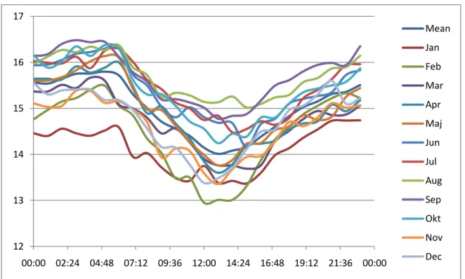
17 Figure 7: Mean Diurnal Wind Profile by Month as evaluated in Windorgrapher – Presented in Excel

Figures 6 and 7 are a representation of the diurnal cycle of wind speeds in Marsabit. Though the range between the highest speed and lowest is approximately 3.5 knots (1.8 m/s), a clear trend is visible where wind accelerates at night having its highest values between 0400 and 0700 hours and the lowest recordings coming in between 1200 and 1600 hours when the sun’s heat is felt most intensively.

Figure 8: Monthly Duration Curve for Marsabit Exported to Microsoft Excel from Windorgrapher 12 13 14 15 16 17 00:00 02:24 04:48 07:12 09:36 12:00 14:24 16:48 19:12 21:36 00:00 Mean Jan Feb Mar Apr Maj Jun Jul Aug Sep Okt Nov Dec 14 14,2 14,4 14,6 14,8 15 15,2 15,4 15,6 15,8 16 1 2 3 4 5 6 7 8 9 10 11 12

Average Monthly Wind Speed for

Marsabit

Average Monthly Wind Speed for Marsabit

(19)

18 In the initial representation of this data on figure 3 and 4, the trend appeared flat because the range in wind speed data is small, approx 1.5 knots.

2.2.2. Voi data

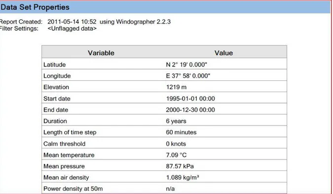
Table 4: Voi Data Properties in Windorgrapher

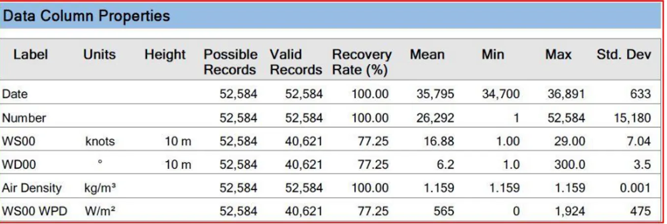
Table 5: Data Summary for Voi in Windorgrapher

In Table 5, the abbreviation WS00 represents Wind Speed in knots and WD00 represents the Wind Direction. WPD means Wind Power Density. Unlike the data recovered from the Marsabit wind records, Voi registers a recovery rate of 77.25%; it is possible to fill the gaps by synthesizing the missing data through windorgrapher by polynomial fit method. Graphs and estimations were made using both synthesized and recovered data and it was found that synthesis lowered the mean wind speed by 0.53 knots at the same time raising the maximum wind speed by 13 knots therefore only the original data with gaps have been presented in this document.

(20)

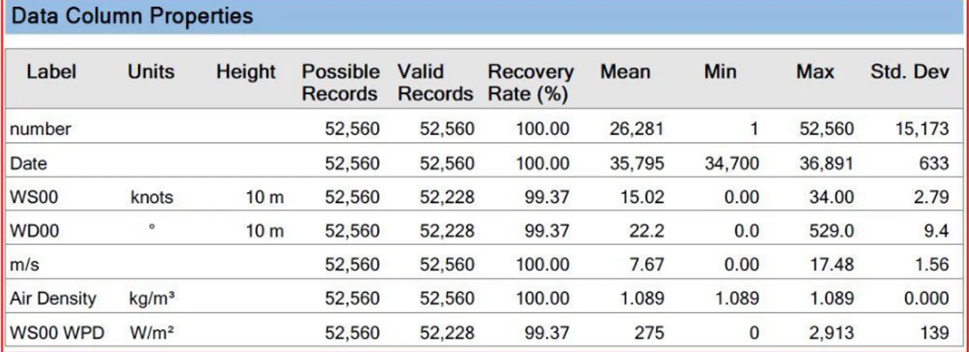
19 Figure 9: Voi Diurnal Cycle by Month – Windorgrapher Interface

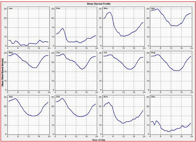
Figure 9 shows the variations in wind speeds in a 24 hour cycle in Voi for every month of the year and averaged over six years. The curves have a similar trend which is visible in figure 10 that is made up from the same results as figure 9 and presented using an excel graph collectively, unlike Marsabit graphs, the highest speeds are logged between 0200 and 0500 hours, before sun rise, while the lowest speeds are experienced between 1500 and 1700 hours.

The influence of the Monsoon winds, described in the first chapter of this thesis, that blow along the East African coast is very apparent at this site as Voi is located less than 200 Km from the coast line. The high speeds logged between April and September are characteristic of the ‘Kusi’ or southerly monsoon winds that carried traders northwards towards Arabia and the lower speeds are recorded during the ‘Kaskazi’ (North-Easterly Monsoon) from December to March. The inconsistency and low speeds could be attributed to the different intensities by which these winds blow. This trend is more visible on the average monthly wind speed graph in figure 11 generated in excel from the data evaluated in windorgrapher. Excel is used due to the clarity in presentation and ease of scale manipulation [10], [14].

(21)

20 Figure 10: Voi Diurnal Wind Profile by Month as evaluated in Windorgrapher

Figure 11: Monthly Duration Curve for Voi Exported to Microsoft Excel from Windorgrapher 2 4 6 8 10 12 14 16 18 20 22 24 26 28 00:00 02:24 04:48 07:12 09:36 12:00 14:24 16:48 19:12 21:36 00:00 Jan Feb Mar Apr Maj Jun Jul Aug Sep Okt Nov Dec Mean 0 5 10 15 20 25 1 2 3 4 5 6 7 8 9 10 11 12

Average Monthly Wind Speed in Voi

(22)

21 Figure 12: Time Series by Monthly Mean Wind Speeds over six years for Voi

Figure 12 is a representation of monthly average wind speeds in Voi for the six year period of data analyzed for this thesis paper. Trends such as these help wind power developers to predict the wind regime for the life cycle of the turbines in their wind park.

2.3. Wind Shear

The effect of the ground friction on wind speed reduces with height, thus the wind is known to gain momentum as you go higher above the ground [37]. The variation in wind speed with height is defined as the wind shear profile or wind speed profile. This varies from site to site depending mostly on the terrain but also on climatic conditions. In order to run accurate simulations for this project, it was necessary to find out the wind shear profile in the region. Unfortunately, we only had wind data for one height, 10m. The WASP simulation model was used in WindPRO software calculate the wind shear coefficient according to power law and logarithmic profiles which can be used as input values n the hybrid optimization models so as to synthesize wind data at any height. Files imported from the 3TIER data resource for wind speeds at 100 meter height were used to calculate the wind shear coefficient as 0.15 according to the power law and the roughness length as 0.03 for the logarithmic profile. Figure 13 is a representation of the result obtained in the WindPRO interface.

(23)

22 Figure 13: Wind Shear Profile from WindPRO and WASP

(24)

23

3. Site Description

In chapter two of this thesis, efforts were made to narrow down the range of site choices based on the wind data provided to us. This helped us eliminate ten out of the twelve locations we started with. This chapter will go on to describe the site chosen out of the winning two.

This thesis is aimed at designing a project that will empower a community, giving them the basic tools necessary to start climbing out of the pits of poverty. We aim to provide a system that gives the residents access to electricity, education, health care, food and water. It is not a hand out system as the overall aim is to spark residual productivity. If the project is attractive it can be turned over to the government or other interested investors. Therefore, it was necessary to propose a site that posed the least complications for the pilot project. Other sites would be considered for application of the same system if it is successful.

It was necessary that the site be easily accessible, both from the sea port, Mombasa and the capital city, Nairobi. Although the project is designed for off-grid systems, we wanted to entice the grid owner to consider connecting the wind farm to the grid sometime in the near future, which would go into ensuring continuity of the project beyond its initial lifespan. For this reason, it was necessary to choose a site that was not too far removed from the electricity grid. There is only one grid owner in Kenya, the Kenya Power and Lighting Company (KPLC) locating such a lucrative venture within their reach would encourage their participation and warrant for development of other similar projects in locations even further away from the grid. It is always more attractive and beneficial to extend the grid to a point of power production rather than consumption. Furthermore, the energy policy in Kenya has limitations as to how much electricity Independent Power Producers (IPPs) can generate without selling it to KPLC which is the only company that has the right to transmit and distribute electricity for sale [18]. Therefore, expansion of the project beyond the setting of this study can only be done in conjunction with the KPLC.

3.1. Location

Voi is a town located in the Taita Taveta district of Coast Province, Kenya, which is in the South Eastern region of the country. At 30 23’ South and 380 34’ East, Voi is 327 Km from Nairobi, the capital city and 160 Km from Mombasa, the country’s main sea port. Road access to Voi is exceptional because the town lies on the Nairobi – Mombasa highway and is the connection point for the road to the Taita Hills and Wundanyi, the district administrative headquarters and leads to a border crossing to Tanzania. The town began as a resting and trading point during the slave trade 400 years ago and grew into modern significance while the Kenya – Uganda railway was under construction at the end of the 19th century [19]. The town is bordered by the Tsavo National Park to the north and east and has thus become a popular hub for tourists and park officials to stock up on supplies. Farmers from the Taita Hills also sell their produce in the town especially to travelers to and from Nairobi or

(25)

24 Mombasa. To the south of the town are the Sagala hills and the Voi Sisal Estates are found west of Voi town. Figures 14 and 15 show overhead maps of the region and give us an idea of the terrain and use of land around Voi town.

Figure 14: Voi Satellite Image

(26)

25

3.2. Lifestyle

The population in Voi municipality in 1999 was 33, 077 and 75% of the residents of Voi are classified as living in informal settlements and of the total housing built in the municipality by 1995, 70% were made from temporary materials [19]. A large number of the residents of Voi municipality are classified as squatters; people living and making use of land that is not registered in their names. The land in question could be owned by the government or other individuals [19]. Apart from the cultivation of sisal in plantations and agricultural activity along the seasonal river banks, subsistence farming is usually carried out during the rainy season once a year and the farmland left bare for the rest of the year.

The Voi town has attracted people from the surrounding regions with better employment and education opportunities. The town has seven primary schools and only two secondary schools. There are three markets in Voi where traders can supply travelers and other tourists who frequent the Tsavo National Park. Other work opportunities are offered by the Voi Sisal Estates and gemstone mining in Sagala hills.

(27)

26

4. Load Simulation

The Load required in an energy system is one of the most vital parameters for its design. The knowledge of how much energy the system must deliver allows the developers to set a lower limit for the project and estimate a preliminary upper boundary. Although this system is being designed for a hypothetical community, the parameters and data must be as realistic as possible.

4.1. Firsthand Information

The preliminary attempt to simulate the electricity load involved sending out requests to a random selection of Nairobi residents asking them to provide information on their annual household electricity consumption in accordance with the electricity bills they received every month. The main reason this town was chosen for this assessment is that Nairobi is the capital city of Kenya and has the best electricity distribution system in the country unfortunately this does not spare residents from frequent blackouts due to load shedding throughout the year. It was still not known which town the project would be done in at the time the questionnaires were distributed because the wind data assessment had not began. It was however certain that the project was to be done in a rural or remote location and the electricity demand in a typical household in Nairobi was expected to be considerably larger than the estimated demand in a typical rural setting due to the differences in usage, nature and type of household appliances and the income levels.

Although the people who received the requests for information were very supportive and held positive attitudes to the task, feedback has been extremely low. Many of the respondents gave reasons that explained this tendency. It was found that most people do not keep their bills after paying them every month let alone for an entire year and secondly, people usually pay attention only to the price on the bill and have a general idea of the price they pay each month, which is hard to use for load estimation since the price per unit varies according to several factors.

Since Kenya does not experience winter and summer, the electricity consumption from month to month does not vary much except for the months of April, August and December when children are on school holidays. This allows us to generate a figure to represent the average monthly electricity consumption and an acceptable range from the data received. Table 6 below shows actual electricity consumption by month from eleven middle and high income households in Nairobi with four to six residents each, letters are used to represent individual households and names are with held for discretion.

The average load per month, obtained from dividing the average monthly consumption of all data sources by the number of sources represented in table 6, has been found to be 240.41 kWh per month and the total annual average electricity consumption amounts to 2832.92 kWh per house per year. It is however speculative to say that these eleven samples are representative for the typical electricity consumption of the country. The aim of this exercise

(28)

27 was to obtain a general idea of some trends observed in the country’s capital. Each of these consumers presents a unique set of characteristics and a considerably larger sample group would be needed so as to group and categorize participants with similarities based on significant levels of criteria such as regional or economical basis; an analysis of this nature was carried out in Kenya in 2005 [5] is discussed in chapter 4.2, next.

Table 6: Electricity Consumption for Typical Nairobi Household in (KWh)

Month A B C D E F G H I J K January 71 100 260 215 670 70 415 97 170 120 312 February 72 66,7 220 230 588 76 378,5 159 173 140,7 357 March 75 106,7 204 315 720 66 710,5 45 172 106 350 April 70 100 282 300 720 66 562 84 177 178 320 May 76 106,7 190 245 554 67 538,5 267 179 155 302 June 78 100 196 345 589 49 469 148 169 135 315 July 81 106,7 272 312 660 67 378,8 220 173 119 394 August 80 113,3 250 285 786 81 457,6 131 181 163 397 September 73 100 237 250 576 76 354,5 118 179 113 380 October 75 106,7 223 215 556 65 521,3 103 175 115 306 November 78 100 230 300 570 72 1062 112 179 163 394 December 83 120 270 276 580 66 623,3 97 180 182 305 Total 829 1106,8 2564 3012 7569 821 5847,7 1484 2107 1689,7 4132 Average 69,1 92,2 213,67 251 630,75 68,41 487,31 123,67 175,6 188,5 344,3 4.2. Secondary Information

Secondary sources of information are usually used to back up research and especially when resources to carry out an extensive study are limited. It is easier to obtain data that suits your study perfectly when you use firsthand information. To ensure credibility and reliability of secondary data you must take the sources into serious consideration. The information that will be presented here is mainly obtained from the Kenya Energy Atlas (2005) [5] and Kenya electricity Generating Company (KenGen) [3].

(29)

28 Figure 16: Average Annual Household Electricity Consumption by Sector in Kenya [5]

The results displayed in the tale in figure 16 indicate that a large scale study was carried out that involved specific inquires that allowed categorization of the target population into two major sample groups according to social setting (Rural and Urban) and further grouping led to the creation of six sub divisions. The first hand information data presented in section 4.1 is insufficient in comparison to this because it only has data collected from the urban areas. However, it has enough information to enable verification of the findings of the secondary data.

If the averages reported in the secondary data correspond to those presented in the firsthand then they can be used to complement each other, if not, then further explanations of the contradictions will be required. This verification of data is very important as it will ascertain that the information on rural electricity consumption is credible and thus suitable for use in this thesis project; more so in the next chapter that is involved with the optimization of the hybrid system.

4.3. Comparison of Primary and Secondary Data

Focusing on the ‘urban areas’ section of the table in Figure 16, we can see that subdivisions have been made in terms of household income bracket. Categories have been made to group high, medium and low income households separately as their electricity consumption behavior is different. As mentioned in section 4.1, data for Table 6 was collected from high and middle income households. The information displayed in Figure 16 also indicates that the average household size in the report is 3.9 while the firsthand data was taken from households with 4 to 6 residents.

(30)

29 Using the criteria from Figure 16 to classify data from Table 6, we can say the consumers A and F are from middle income households while the other ten are high income households. The high margin displayed with consumers D, E, G and K can be attributed to the number of residents in the house being six. The difference in average annual electricity consumption between Table 6, 2832.93 kWh and Figure 16, 844 kWh can also be explained by the fact that about 80% of the data collected for Table 6 is from high income households and none is from low income (as categorized by the secondary data grouping system in figure 16 [5]) thus the results are not representative of all groups of urban dwellers.

From this comparison, we concluded that using the reports depicted in Figure 16 will not compromise the results of this study and will present figures that are realistic and credible. Our project is being designed for a rural community and takes 500 households with 5 residents each. From chapter 3, we can tell that Voi qualifies as a medium to low potential rural zone; household consumption will thus be an estimate between 541 and 672 kWh/house/year according to figure 16. The average household consumption in the table on figure 16 is designed for 4.4 to 4.8 residents, in order for the data to be representative of five residents, in middle to low potential zone the results need to be scaled up.

Where,

ER – Expected number of residents per household

AR – Lower limit of Average number of residents per household S. f – Scale factor

KWh/hse/yr Where,

AEC – Lower limit on Average Electricity Consumption per household per year EEC – Expected Electricity Consumption per household per year

From these calculations, we conclude that the load per house hold per year will be 616.74 kWh. However, this is not the entire load of our system. In Chapter one, the project was described as having a school, a clinic and an irrigation system. These are elaborated in section 4.4 of this thesis.

(31)

30

4.4. Total load definition

The information in part 1, 2 and 3 of this chapter has made it possible to calculate the primary load for one of the 500 households that will be served by this project. In this section we will define the load that the entire system is required to meet. Unfortunately, specific data on the most efficient equipment necessary and their current market values has been difficult to obtain, thus most of the information has been derived from a similar study carried out for Ethiopia that was done in March 2009 [11]. The system in the Ethiopian case was designed to combine solar P.V., wind, diesel and batteries so as to supply a community of 200 families of 5 members each in a remote off-grid location. The load estimated for the school and clinic as well as water supply system for the residents has thus been scaled up to cater for 500 families. The prices and types of the generators and batteries used in the system have been duplicated for use in this thesis project by scaling where necessary. The scale factors on price and choice of equipment is discussed in chapter five of this study. 4.4.1. Primary Load

The Primary load is defined as the electricity demand that must be met immediately it arises; these include lighting, refrigeration, cooking and other household applications. Since the individual house hold load has already been determined in part 4.3, we will look at the load required for the school and clinic. Before describing the load designation for the various sectors in this community, it is important to bear in mind that this thesis main focus is to supply the electricity and recommend a basic system of usage. The system is not absolute and further research will lead to a more refined assignment of load.

4.4.1.1. School Load

Education is essential for community building. Through the school, the residents can receive both formal and practical education, including education for sustainable development. In order to effectively cater for the amount of children estimated in this community, it is assumed that all the three children of each family are of school going age. The classes will be designed to accommodate a maximum of 30 students each. This requires the school to have 50 classrooms and an administration block.

Kenya has the advantage of having an average of 12 hours of sunlight all year round; therefore the electricity consumption of the school is greatly reduced. During the day, electricity usage will be confined to the administrative functions such as running of computers and printers. The bulk of the load will be taken on in the evening as the school will double up as an adult education facility, teaching a wide range of skills to the mature members of the community. These classes would be carried out from 1800h to 2100h. On the load simulation for the school, it is assumed that all the 50 classes plus 1 administrative office will have their lights on for the 3 hours in which the adult classes are going on. This assumption is used to cater for the electric load taken by the administrative buildings during the day as it is clear that the adults would not fill any more than ten classrooms during the evening classes. Each class will be considered to have one 40W bulb

(32)

31 and an option of using equivalent energy saving lights rated at 11W for the same luminance will be explored to reduce the load.

4.4.1.2. Clinic

The clinic will be a basic facility treating day patients and minor ailments. It will work as a health post, stocking medical supplies and documenting the health of the residents. The largest load will be incurred by the freezer that will be used for storing refrigerated medicine; a 70W machine [20] is used as an example in this case and is expected to run for 24 hours a day which gives us 1.68kWh/d.

The clinic will not be able to cater for major ailments or emergencies requiring hospitalization but will rather transfer the more serious cases to larger facilities in Voi town. The clinic will also need to have computers, fax and laboratory equipment to carry out tests and sterilizing apparatus; therefore the load is estimated to be 3kWh/d as shown in Table 7.

Table 7: Projected Primary Electricity Load

Primary Load kWh/d kWh/month kWh/d holiday month

Clinic 3 90 houses 845 25698 school A (40W bulbs) 5,1 153 school B (11W bulbs) 1,403 42,075 total A 853,1 848 total B 849,403 844,303 4.4.2. Deferrable Load

A deferrable load is also known as a secondary load, it is met only after the primary load has been satisfied except under special circumstances. The deferrable load includes activities like pumping water, charging batteries and fly wheels and heating water. Due to the nature of the load, it also determines the energy storage capacity of a system. The storage capacity can be described as the amount of electricity required to fully satisfy the deferrable load in some specific cases; if, for example, the deferrable load comprises the pumping of water into a tank, the storage capacity will be the amount of electricity required to fill it because the electricity can be used for other purposes until the tank is empty. The special circumstances mentioned at the beginning of this paragraph include cases when the water tank or batteries are empty or below the acceptable level.

4.4.2.1. Water Supply

The quality of life is greatly improved by household access to clean water. This system aims to provide clean water to the houses, school and clinic on a daily basis. In this case, the study carried out in Ethiopia, Bekele & Björn (2009) [11], is our point of reference. A more practical study at the site would allow the assessment of locally available equipment and suppliers may yield more appropriate results. This system, designed for 500 households, uses 18

(33)

32 pumps with a power rating of 150W each to supply each house with 108 liters of water a day. The water is pumped at a rate of 10 liters per minute for five hours every day. These figures are clearly represented in Table 8.

The water supply to the school and clinic is not as much as the amount needed by the households and is thus considered together as one load. For simplicity of design and supply of equipment for the project, it is better to use the same kind of pump in the entire system. Three pumps, run for four hours daily, are to be used to supply water to the school and clinic. This will provide 7200 liters of water per day.

4.4.2.2. Irrigation System

Agricultural productivity in Voi is limited by the aridity of the region. The three month rainy season from September and November is not enough to encourage significant advances in the economical status of the residents. The seasonal river a few kilometers north of Voi town waters the region for a while but the technology required to maximize the water available in the rainy season is still lacking. Many communities in Kenya are being encouraged to turn to artificial irrigation systems to grow their food crops [21] especially with the recent prolonged droughts that have threatened food security nationally. A good reliable irrigation system will enable residence to begin to be self sufficient by growing their own food and at the same time, allow them to earn money from sales; in this way, the project becomes more profitable and payback time can be shortened.

A Drip Irrigation System has been chosen for this particular pre feasibility study. The intricacies of design will not be looked into with much detail due to limited time nevertheless, an overview will be sufficient for this study as the thesis will focus on the amount of electricity required to run the system. A drip irrigation system is designed for operation in regions with limited water supply and high evaporation. The system is comprised of a network of pipes equipped with emitters at given distances that let water out in drops intermittently at the base of a plant. The simplest applications require a reservoir to be placed at a considerable height above the farm land so that the water can be distributed by gravity and thus save costs [22]. The amount of water reaching the plants is regulated by taps at various points in the pipes. Sophisticated systems have regulation at every water emission point while others are just rubber pipes with holes made at predefined distances. Large systems like plantations require pumps to distribute the water. Pumps are also used when the water source is a river or lake, as they are on the same level as the farm. A drip irrigation system saves a lot of water [23].

The electricity directed for use in this drip irrigation system is to be used for pumping water into the irrigation reservoirs or tanks. 6 pumps just like those described in part 4.4.2.1 of this thesis will be incorporated into the hybrid system to supply 7200 liters of water per day to the irrigation system tanks. These pumps will run for a total of two hours daily and consume about 1.8kWh/d. Table 8 shows a numerical breakdown of the electricity load. Note that the deferrable load reduces from September to November because it is the rainy season and the

(34)

33 irrigation system pumps are not used at all while the water supply pumps work for fewer hours.

Table 8: Projected Deferrable Electricity Load

Demand Number of Pumps kWh/d KWh/m storage (kWh) peak (kW)

Houses Water Supply 18 13,5 405 60 2,7

Clinic & School Water 3 1,8 54 7,2 0,45

Irrigation System 6 1,8 54 8 0,9

(35)

34

5. The Hybrid System

The use of the term ‘Hybrid System’ when referring to generation of electricity points to a system that uses more than one power source to produce electricity [20]. A hybrid system usually consists of one or more renewable energy sources and is common with isolated power systems and weak grids. The most common hybrid combinations are PV-Diesel and Wind-Diesel [34]. One of the reasons it is attractive to use hybrid systems for off-grid applications is for power balancing; most renewable energy sources have a fluctuating energy output and need a consistent power source to kick in when the levels of renewable energy output goes down thus avoiding flicker and blackouts. Simple hybrid systems use batteries for immediate response to reduction in power output and diesel generators for longer lasting situations. An immediate response or primary control refers to a loss in power that needs to be countered in a matter of seconds before its effect is felt by the consumers while a longer lasting situation requires secondary control which employs mechanisms like the Automatic Generation Control (AGC) that is designed to kick in if the interruption in power delivery is not abated in about 10 - 15 minutes [24]. Prediction of a drop in power production by one energy source helps system operators to structure the hybrid model to begin firing up back up power well in advance.

5.1. Hybrid Modeling and Optimization

The modeling of hybrid power systems can be a complex and time consuming task due to the various uncertainties involved. In order to obtain accurate and reliable results, a lot of care and attention must be paid while collecting and compiling data. The hybrid modeling and optimization software, HOMER [25], helps the modeler to run as many design options as required. The system designer can introduce several variables and HOMER will run all the possible simulations and deliver results in easy to read tables and graphs. HOMER carries out operations such as simulation, optimization and sensitivity analysis when data is introduced. The software uses data from manufacturers of wind turbines, batteries, generators and all other power generating equipment that the modelers may choose to have in their system. This information is used in conjunction with the input data concerning the electricity load and resource availability such as solar irradiation or wind speeds, to synthesize a set hybrid model options that meet the requirements of the system.

The software also runs optimization models and the results are displayed according to the least cost of energy (COE) or any other criteria selected. The sensitivity analysis allows the modeler to explore various possibilities in consideration of all the variables that could come into play during the life cycle of the power system. All values that cause uncertainty can be varied to find the best and worst case scenarios in which the project would be feasible. One could introduce variable prices of fuel for example, variable wind speeds or solar irradiation levels, variable hub heights and types of wind turbines and so on. Varying parameters like this can help a project developer to simultaneously obtain results for different sites of

(36)

35 interest that have the same general setup especially in cases where the annual average wind speed or solar irradiation is the only difference. The results of the sensitivity analysis help the developer to choose the most desirable system from a reasonable range of viable scenarios.

The results obtained from HOMER are directly dependent on the input data which needs to be as accurate as possible. This is in especially true for capital and operation costs of equipment in the system. Some of this data such as costs of wind turbines is not easily accessible to developers. Therefore, developers usually try to overestimate so as not to fall short of investment targets. Updating the simulations according to new data obtained is very simple. The software does not require a user to be an expert in any electrical field as the interface and guides for usage are very comprehensive. More details on the operation of HOMER will be discussed in the hybrid set up description.

5.2. Hybrid Setup

The results obtained from HOMER’s simulations are most sensitive to input data. This section of the thesis will go into the description of input variables and the requirements of the software in each case. Details on specific input values have been discussed in previous chapters and will only be mentioned here.

5.2.1. Input Values 5.2.1.1. Load

The electrical load is the first value to be introduced to the software. This helps us to select the equipment necessary to meet the load. HOMER is able to determine whether the equipment is sufficient to meet the load or not.

The primary load needs to be described on an hourly basis, so that the software can model the peak load and low consumption hours. This helps in selecting the most economical power source according to power consumption. Specific data on electricity consumption per hour is usually available if a power system is currently running and the hybrid system is being applied to help reduce the cost of electricity. As an example, a system that is run totally on diesel generators can be altered to include alternate energy sources such as wind or solar. In cases where the particular consumption is not known for every hour, the software uses a default diurnal load profile which the modeler scales up or down by entering an annual scaled average load measured in kilowatts per day. This is the estimated value of the primary load for one day. The 24 hours load profile from HOMER was scaled up by an annual scaled average of 843 kWh, the daily primary load under consideration for this project.

The deferrable load, on the other hand is introduced on a monthly average basis rather than an hourly one. The least amount of power necessary to meet the load is known as the Minimum Load Ration and is specified as a percentage of the peak deferrable load defined in chapter 4.4.2. The default minimum load ratio value for water pumps in HOMER is 67%.

(37)

36 Figure 17 and 18 below show images from the HOMER interface for the primary and secondary load input data.

(38)

37 Figure 18: Secondary Load Input Data in HOMER Interface

5.2.1.2. Equipment to Consider

The power sources used in the hybrid system are chosen according to the project developer’s preference. For this case, wind turbines, diesel generator, batteries including an energy converter with the capacity to act as both an inverter (DC to AC) and a rectifier (AC to DC) to help propagate energy through the entire system easily were chosen.

(39)

38 5.2.1.2.1. Diesel Generators

The diesel generator in this hybrid system acts as the secondary power source. It is set to support the wind turbine generators when they are not producing enough electricity to meet the load. Diesel generators are cheaper to install but have higher operational costs than the wind turbines and batteries therefore they are run for as few hours as possible. One diesel generator was chosen and different sizes were considered for simulation, from 0 – 300 kW. This allows the software to select the most economical generator capacity for the system. The capital cost for the generator was set at 1500 USD per kW, cost of replacement at 1200 USD per kW and 0.05 USD per hour is the operation and maintenance cost excluding fuel cost [33]. Figure 20 shows the main input data for the diesel generator chosen for this system.

Figure 20: Diesel Generator Inputs

5.2.1.2.2. Wind Turbines

There is a wide range of turbines that could be used for a project such as this. HOMER makes it possible for a modeler to either use wind turbine data available in its files or introduce new wind turbine information and their respective power curves. A power curve is a graph showing the amount of electricity generated by the turbine in relation to the wind speed. After a few simulations, it was found that turbines with more than 100 kW power rating generated more power than the project needed; systems with only one wind turbine

(40)

39 produced up to 80% excess energy. Furthermore, the simulations only required one wind turbine. Instead of using one turbine of high rated power, turbines with lower power rating were considered and this proved to reduce the cost of electricity per kilowatt hour and reduce losses due to excess electricity generation. The cost of load shedding was not considered. The generic 20kW model from HOMER and the Fuhrländer 30kW turbines were used for the consequent simulations. Figure 21 and 22 show details about the wind turbines considered for this project. Figure 21 shows a generic 20 kW turbine used in a previous study similar to this thesis [11] while figure 22 shows details on a Fuhrländer 30 kW wind turbine that was chosen as the primary turbine for this project.

Information on the cost of wind turbines is not easily available except when making actual purchases. Estimations of the cost of capital, replacement and operation and Maintenance were made using data from the Canadian Wind Energy Association [26] and the study carried out for a similar hybrid system in Ethiopia by Getachew & Björn (2009)[11]. The two sources made it possible to set an upper and lower limit to turbine cost and obtain the optimum system for both cost categories.

Table 8: Cost estimates for Wind Turbines

Cost Limit Capital Cost $/kW Replacement Cost $/kW O & M $/yr

Upper Cost Limit [5] 4000 2500 100

Lower Cost Limit [11] 2250 1500 45

(41)

40 Figure 22: Fuhrländer Wind turbine Input Data

5.2.1.2.3. Batteries

The batteries in a hybrid system work as reserve or back up energy. They are charged when the electricity produced in the system is greater than the load and discharged when the demand is higher than the power generated. Since the batteries have lower operation costs than the diesel generators, they are usually charged using electricity generated by the wind turbines except when they are below allowable limits. The allowable limits for the batteries (or set point state of charge) are defined as part of the dispatch strategy which is discussed under the system control inputs. The Surrette 6CS25P battery was chosen for this project because its financial information was available and results of its operation in a hybrid system could be accessed [11]. The capital cost input is assumed to cover all mounting, installation and labor costs related to the batteries’ acquisition [11], [25]. In this case, the capital and replacement costs for one battery were 833 USD and 555 USD respectively while O&M costs were 15 USD per year [11]. The default minimum battery life for Surrette 6CS25P that is considered by HOMER is 4 years and is thus used in this study. Figure 23 shows the input data for the battery used in this project.

(42)

41 Figure 23: Battery Input Data

5.2.1.2.4. Converter

The converter is necessary when a power system requires the conversion of alternating current AC to direct current DC or vice versa. If both conversions are needed, the converter acts as both an inverter (DC to AC) and a rectifier (AC to DC). The capital and replacement costs for the converter were taken as 7 USD per kilowatt and lifespan as 15 years [11]. The input data for the converter used in this project is shown in figure 24.

(43)

42 Figure 24: Converter Input Data

5.2.1.3. Resources

The calculation of power output requires data concerning the resource available to run the system in relation to your choice of equipment. Each resource has a special set of information needed for simulation which is expounded upon in this section.

5.2.1.3.1. Wind Resource Input Data

The software uses wind speed data to calculate the output of the wind turbines in your system as well as determine when alternative power sources are required to help meet the demand for electricity. The wind data can be imported directly into the software as hourly measurements for one year as a time series data file or monthly averages can be added manually into the input interface. Monthly averages were used in the simulations. Figure 25 shows the overall input data for wind resource, the simulation also takes the height above sea level and the height at which the measurements were taken into account.

(44)

43 Figure 25: Wind Resource Input Data

The variation with height tab in the centre of figure 25 allows a system modeler to give information that helps define the wind speed profile for software calculations. The software uses either the power law or logarithmic wind speed profile in calculations so to estimate wind speed variation with height. Figure 26 and 27 show the options available when defining wind speed profile. Simulations were done for 25, 30 and 40 meter hub heights and will be presented in the results section of this chapter.

(45)

44 Figure 26: Wind Speed Variation with Height; Power Law Profile

Figure 27: Wind Speed Variation with Height; Logarithmic Profile

5.2.1.3.2. Diesel Input Data

The resource information required for calculation of generator output concerns the fuel to be used. In this case the fuel chosen was diesel and a price range was introduced to compute the price at which running the generator becomes uneconomical. The price of diesel in Nairobi at the end of April 2011 was set at 107 Kenya shillings which translates to 1.24 USD,

(46)

45 this was a reduction from 120 Kenya Shillings (1.38 USD) the previous week [27]. The range of values considered for the price of diesel per liter in this project is from 1USD to 1.5 USD.

Figure 28: Fuel Resource Input Data

Figure 29: Price Range of Diesel $/L

5.2.1.4. Other Parameters

The parameters in this sector help in defining how the calculations are done. They cover the Economics, System Control, Emissions and Constraints of the hybrid system. The Economics section covers interest rates and helps in the calculation of net present value. The emmissions section lets the developer calculate the amounts and consequent penalties of hazardous gases emitted by the power system. Models that exceed acceptable limits are