Research
3D Thermo-Mechanical Coupled
Model-ling of Thermo-Seismic Response of a
Fractured Rock Mass related to the
Final Disposal of Spent Nuclear Fuel
and Nuclear Waste in Hard Rock
SSM perspective
BackgroundWhen assessing the long-term safety of a repository for spent nuclear
fuel it is important to consider future earthquakes. Previous studies by
Yoon et al. (2014, SSM Report 2014:59) and (2016, SSM Report 2016:23)
investigated the fracture responses due to heat and earthquakes at
major deformation zones using a 2D thermo-mechanical coupled model
that uses a Particle Flow Code (PFC2D, Itasca). The 2D approach limits
the investigation to horizontal and vertical cross sections of the
Fors-mark site and the model is not able to handle interactions of steeply
dip-ping and gently dipdip-ping faults. Thus, the 2D approach is not capable to
address the question if an occurrence of an earthquake at a gently
dip-ping fault, could reactivate some of the large, steeply dipdip-ping faults. To
explore thermally and/or seismic induced fracture slip of the repository
fracture system, this study was performed with 3D thermo-mechanical
coupled modelling using Particle Flow Code 3D v4 (PFC3D v4).
Impor-tantly, before the 3D thermo-mechanical coupled modelling could be
performed, a 3D geological model of the Forsmark site had to be created
representing the repository fracture system and relevant deformation
zones.
Results
The aim of the research is to explore 3D earthquake simulation and the
heat load from the spent nuclear fuel and its potential impact on the
repository fracture system. Three scenarios were investigated:
• heating scenario, heat load inducing repository fracture slip
• earthquake scenario, seismic load inducing repository fracture slip
• earthquake scenario under thermal phase.
The simulated impact of the heat generated from the deposited spent
nuclear fuel induces slip in the repository fracture system. Further, the
fracture dilation during the heating is irreversible.
The scaling parameters of the simulated fault rupture agree well with
the earthquake fault empirical scaling relations. Coseismic slip
distri-butions of the activated faults show triangular and asymmetric pattern
and sharp increase/drop of displacements at the location of
intersec-tion with neighbouring faults. The results show high resemblance to the
observations of slip distribution of natural earthquake faults. The results
demonstrate that the workflow Yoon et al. developed for simulation of
dynamic fault rupture (earthquake event) based on the discrete element
model and PFC3D v4 well capture the characteristics of the natural
earthquake faults. The performed modelling shows that, under
pre-sent day stress conditions, the secondary fracture displacement in the
repository volume due to seismic loads is more sensitive to the distance
where the primary seismic fault occurs than to the size of the primary
seismic fault.
The performed modelling also shows that the impact of an earthquake
event occurring during the early time of repository heating (50-100
years) amplifies the shear displacements of the repository factures by a
factor of 10 to 1000 compared to shear displacements induced by the
heat load alone.
Relevance
Canister failure due to shear load is included in SKB’s main scenario
for the safety case for the planned repository for spent nuclear fuel in
Forsmark. Thus, it is important to understand possible causes for shear
movements in the repository volume and the response of the canister to
these movements. This study explores how:
• repository fracture behaves under the influence of heat loads
• repository fracture behaves under the influence of seismic loads
• repository fracture behaves if an earthquake coincides with the heat
load.
Therefore, the study is important for SSM’s understanding of shear
move-ments in the repository volume and their impact in the continued review
of SKB’s application for a spent nuclear fuel repository in Forsmark.
Need for further researchThe PFC3D v4 simulations resulted in unexpected large fracture slip in
the repository volume compared to the PFC2D simulations. The reason
for this needs to be explored in future research. The thermal modelling
can potentially be improved by comparing the PFC3D v4 thermal
mod-elling results with published analytical close form solutions. In
addi-tion, the far field response to the heating of the repository should be
included in future work in order to examine how the heat is dissipated
in the model. Further work is also required in the model to define the
damage zone and fault core, which were not done in this study. When
modelling the fault stability during future glacial cycles, further work
is also needed to include the impact from fluid pressure on the fault
activation.
Project information
Contact person SSM: Carl-Henrik Pettersson and Flavio Lanaro
Reference: SSM 2014-3668 / 3030045-14
2019:15
Author: Mattias Thuvander
Department of Applied Physics Chalmers University of Technology
3D Thermo-Mechanical Coupled
Model-ling of Thermo-Seismic Response of a
Fractured Rock Mass related to the
Final Disposal of Spent Nuclear Fuel
and Nuclear Waste in Hard Rock
Project Final Report
3D Mechanical Coupled Modelling of
Thermo-Seismic Response of a Fractured Rock Mass related to the
Final Disposal of Spent Nuclear Fuel and Nuclear Waste in
Hard Rock
Jeoung Seok Yoon, Arno Zang
Helmholtz Centre Potsdam
GFZ German Research Centre for Geosciences
Potsdam, Germany
September 2019
Reference number: SSM2014-3668 Project number: 3030045-14
Contents
Executive Summary ... 4
1. Project introduction ... 6
1.1. Background ... 6
1.2. Objectives ... 7
1.3. Work packages and the structure of the report ... 7
2. Summary of previous studies ... 8
2.1. SKB-Posiva modelling studies ... 8
2.2. SSM’s modelling studies ... 9
3. Seismicity in Sweden ... 11
3.1. Spatial distribution of seismicity ... 11
3.2. Future earthquake probabilities ... 11
3.3. Summary and Discussion ... 13
4. Geological model of Forsmark repository site in 3D ... 15
4.1. Local and Regional Scale Models and the deformation zones ... 15
4.2. Repository discrete fracture system ... 20
4.3. Repository panels... 25
4.4. In-situ stress and its evolution during glaciation ... 29
4.5. Dynamic fault rupture ... 32
5. Analysis of fracture shear displacement ... 35
5.1. Shear displacement of a single fracture in continuum model: FRACOD2D analysis ... 35
5.2. Fracture shear displacement of a fracture in a discontinuum model: PFC3D analysis ... 38
5.2.1. Effect of smooth joint resolution on shear displacement ... 38
5.2.2. Effect of rattlers on shear displacement ... 40
5.2.3. Effect of fracture embedding sequence on shear displacement ... 44
5.3. Comparison of shear displacement: multiple segmented representation vs. single planar idealization ... 47
5.4. Discussion ... 49
6. Modelling cases ... 55
6.1. Local Scale Model (LSM) ... 55
6.2. Regional Scale Model (RSM) ... 55
7. Modelling of repository heating and the impact to the
repository fractures ... 57
7.1. Spatio-temporal distribution of rock temperature increase ... 57
7.2. Thermally induced repository fracture shear displacement ... 61
7.3. Summary and discussion ... 62
8. Modelling of fault activation and the impact to the repository
fractures ... 66
8.1. Local Scale Model Simulation ... 66
8.1.1. Activation of ZFMWNW0809A under present day in-situ stress condition ... 66
8.2.2. Activation of ZFMWNW0001 (Singö fault) under glacial ice
cover forebulge stress condition ... 70
8.2.3. Activation of ZFMA2 under present day in-situ stress condition ... 72
8.2.4. Activation of ZFMA3 under present day in-situ stress condition ... 74
8.2.5. Activation of ZFMA3 under glacial ice cover retreat stress condition ... 76
8.3. Summary and discussion ... 78
9. Modelling of fault activation under repository heat and the
impact on the repository fractures ... 87
9.1. LSM – Activation of ZFMWNW0809A under present day in-situ stress condition and after 50 years of simultaneous panel heating ... 87
9.2. LSM – Activation of ZFMWNW0809A under present day in-situ stress condition and after 100 years of simultaneous panel heating ... 88
9.3. Summary and discussion ... 89
10. Discussion ... 91
11. Recommendations for further study ... 95
12. Conclusions ... 99
13. Acknowledgement ... 101
Executive Summary
In this numerical modelling research project, we investigated the impacts of possible sources of loading on the safety of the proposed underground repository at Forsmark Sweden for final disposal of spent nuclear fuels.
We discuss three sets of scenarios where the long-term safety of the repository can be affected. Firstly, the heat generated from the canisters containing the spent nuclear fuels is considered and results in repository rock mass expansion,
displacement of the repository fractures and possibly reactivation of nearby faults. Secondly, an earthquake event at nearby large deformation zones is considered which generate a seismic loading on the repository rock mass. Thirdly, an
earthquake event occurring during the time when the repository rock mass is under heating is considered.
A three-dimensional discrete element modelling code, Particle Flow Code 3D v4 (PFC3D v4) is chosen for the simulation. The code enables modeling of thermo-mechanical coupled process (conductive heat flow, resulting rock expansion and therefore thermal stress) and dynamic fracturing process (seismic wave generated from a rupturing source propagates and attenuates). Moreover, the code enables implementation of discrete fracture network in a heterogeneously modelled rock mass. Therefore, a discrete fracture embedded in the model is also heterogeneously represented. The fault damage zone is mimicked applying smooth joint contacts.
We studied the possible impacts of the heat loading to the repository fracture system. To do so, we developed a thermo-mechanical coupled simulation workflow and conducted two end-member disposal scenarios: deposition of all canisters and closure at the same time, deposition of canisters in panel-by-panel sequence. We studied the possible impacts of the earthquake events (dynamic fault rupture) occurring at large deformation zones near the repository site. To simulate a fault rupture with magnitude close to 6 or larger, we generated a large geological model of Forsmark site where the major deformation zones that are well-known by the site investigation are included and represented heterogeneously. In the earthquake modelling scenarios, the considered time span extends to 70k years from present to
take into account of possible changes in the in-situ stress field affected by future
glaciation and deglaciation. In particular, we studied the impact of nearby gently dipping fault located above the repository rock volume when it ruptures under glaciation and deglaciation periods. Lastly, we studied the impact of a nearby fault rupture during the time of the repository heating.
From the heating scenario, it is found that the repository fracture system undergoes heat induced slip which show rapid increase of those repository fractures located within the repository panel rock volume during 50-100 years. The fracture system located outside the repository panel rock volume then slip slowly after 100 years as the generated heat propagates. We found that the fracture slip is irreversible and we interpret that it is due to dilatational behavior of the fractures that are intersected by one another.
From the earthquake scenario, it is found that the seismic impact to the repository fracture system is large when the steeply dipping deformation zone undergoes strike-slip faulting during the glaciation period. We interpret that it is due to
due to unloading of the overburden stress by ice sheet melting which results in stress state more favorable for reverse faulting. Therefore, climate change can have an impact on the long-term safety of Forsmark repository.
From the earthquake scenario under thermal phase of the repository, it is found that the repository fractures slip less, possible due to the disturbed stress field by the heating.
We studied the source parameters of the simulated fault rupture and compared with empirical scaling relation of natural earthquake faults. It is found that the rupture parameter, e.g. rupture area, moment magnitude and slip, agree well with the empirical scaling relation of natural earthquake faults. Moreover, fault slip distribution undergoing dynamic faulting shows asymmetric and triangular pattern and sharp slip contrast at the location of intersection with neighboring faults as can be observed in natural earthquake faults. This result is in contrast to symmetric fault slip profiles simulated in other studies where the fault is represented as a planar structure embedded in an elastic rock body. The results demonstrate that the workflow we developed for simulation of dynamic fault rupture (earthquake event) on the basis of discrete element model and PFC3D v4 well captures the
characteristics and mechanics of the natural earthquake faults.
All the results of earthquake scenarios assume activation of faults that are close to the repository site (hypocenter distance < 5 km from the repository rock volume). It should be noted that the probability of occurrence of earthquake at those faults is very low.
1. Project introduction
1.1. Background
To be able to assess the long term safety of a repository for disposal of radioactive wastes and spent nuclear fuels, it is necessary to consider all possible threats that could impair the physical integrity of the disposal facility. First type of the threat is environmental, which is an earthquake event. The effect of an earthquake relevant to the repository safety is the earthquake induced shear displacement of a rock fracture crossing the deposition borehole containing the nuclear waste canister. Second type of threat is man-made, which is the heat generated from the nuclear wastes. After the nuclear waste canisters are disposed underground, it results in thermal expansion of the repository rock mass and induces shear displacement of the rock fractures crossing the deposition borehole containing the nuclear waste canisters.
It is therefore necessary to estimate the impacts of both the heat (man-made) and earthquake (environmental) that can possibly occur at nearby fault system. To do so, one should rely on a simulation tool that can capture the thermal-mechanical and dynamically coupled processes. Moreover, to be applied to a safety analysis of an underground nuclear waste repository site, the simulation tool should be able to model complex geological system of the site, in particular, heterogeneity of the rock mass and the geological discontinuity system in various scales.
Lately in Sweden in 2011, the Swedish Nuclear Fuel and Waste Management Company (SKB) has submitted an application to the Swedish Government to obtain a construction license for a final repository for spent nuclear fuels at Forsmark. The application is currently under regulatory review by the Swedish Radiation Safety Authority (SSM) and by the Land and Environmental Court (Lanaro et al. 2015). Yoon et al. (2014, 2016a, 2016b, 2017) have investigated the safety of the Forsmark repository against the heat generated by the disposed spent fuel and the earthquake events occurring at nearby faults by conducting 2D discrete element-fracture dynamic modeling using Particle Flow Code 2D version 4 (PFC2D v4). The key results of the two studies of Yoon et al. (2014, 2016a, 2016b) are summarized in Chapter 2.
In this project, we extend this modelling studies of Yoon et al. (2014, 2016a, 2016b) into a 3D setting. Compared to the previous studies, the model is enlarged in order to investigate the impacts of larger magnitude (Mw >6) earthquakes that may occur at large deformation zones near the Forsmark repository in the next few hundred years and during future glaciation.
To be comparable with previous 2D modelling results, we chose PFC3D v4 instead of PFC v5. The reason for use of a discrete element code is that it is able to simulate rock heterogeneity, complex brittle rock fracturing processes under different source of tectonic loading. Moreover, the discrete element code, PFC3D, has a significant advantage, in particular in our application, that structural complexity of the discontinuities in various scales (m-scale repository fractures and km-scale faults) can be embedded in a discrete element rock model.
1.2. Objectives
The objectives of the project are the followings.
(1) Generate a 3D geological model of Forsmark repository site with
heterogeneously represented geological discontinuities;
(2) Investigate the impacts of the heat generated by the spent nuclear fuels to
the repository fracture system;
(3) Investigate the impacts of magnitude, M> 6 earthquakes at nearby large
deformation zones to the repository fracture system;
(4) Investigate the impacts of glaciation to the earthquake events and to the
repository fracture system;
(5) Investigate the combined impact of an earthquake and the heat to the
repository fracture system;
(6) Validate the simulated earthquake source parameters against empirical
scaling relation of natural earthquake faults.
1.3. Work packages and the structure of the report
To achieve the above objectives, the project is divided into several work packages (WPs) which are the followings.
WP1: Generation of discrete element based 3D geological model of Forsmark repository site with heterogeneously modelled geological discontinuities (deformation zones and repository fracture system);
WP2: Analysis of the response of the repository fracture system induced by thermal loading;
WP3: Analysis of the response of the repository fracture system induced by fault dynamic rupture;
WP4: Analysis of the response of the repository fracture system induced by combined thermal loading and fault dynamic rupture;
WP5: Analysis of the shear displacement of single isolated and intersected fractures that are represented by smooth joint contact model in a discrete bonded particle model.
Chapter 2 summarizes the previous studies conducted by SKB-Posiva and SSM. Chapter 3 reviews seismicity of Sweden. Chapter 4 describes the development of the 3D geological model (WP1). Chapter 5 presents the concept of shear displacement analysis in this study (WP5). Chapter 6 lists the modelling scenarios. Chapter 7 describes the WP2 and compares the results with those of 2D modelling study by Yoon et al. (2016a). Chapter 8 presents the results of WP3 and also compares the results with those of 2D modelling studies by Yoon et al. (2014, 2016a, 2016b, 2017). Chapter 9 presents the results of WP4. In Chapter 10, we discuss several issues related to the comparison between the previous modelling studies and possible uncertainties in the results. Chapter 11 recommends several issues that are recommended for further study. Chapter 12 represents the conclusions of the study.
2. Summary of previous studies
2.1. SKB-Posiva modelling studies
There has been a number of modelling studies investigating the impacts of
earthquake events to the repository fractures. The most relevant studies are by Fälth et al. (2010, 2015) for SKB and Posiva (organization responsible for the final disposal of spent nuclear fuel in Finland) where they used 3DEC (Itasca’s three-dimensional distinct element code) and investigated the following questions:
What are the static and dynamic impacts of an earthquake upon nearby
fractures in terms of induced shear displacement?
How does the induced shear displacement correlate to the distance from
and the magnitude of the seismic source?
The earthquakes simulated were of reverse faulting type, but the SKB studies did not try to reproduce an expected typical post-glacial faulting event at Forsmark,
Oilkiluoto or Laxemar. Instead, input data that control potentially important seismic parameters such as event magnitude and amount of stress drop are varied
systematically in generic simulations to cover event ranges that are potentially relevant to the safety assessment.
To simulate an earthquake event, the fault rupture was initiated at a pre-defined location and programmed to propagate outward along the fault plane with a specified rupture velocity until the propagation is arrested at a the rupture area boundary. The models include large numbers of explicitly modelled host rock fractures with varying orientations at different distances from the earthquake fault as shown in Figure 2-1. The coseismic response of these target fractures, i.e. the induced target fracture slip, was the main outputs of their simulations.
The dynamic 3DEC simulations reported by Fälth et al. (2010) are briefly described as follows:
Earthquakes were simulated on schematic, hypothetical, rectangular fault
plane without couplings to the Forsmark site or to any other site.
The area of the earthquake hosting faults range between 10 and 1000 km2
. In all cases, the entire fault area was activated (rupture area = fault area), and the moment magnitudes (Mw) ranged between 5 and 7.
Stress fields were defined without couplings to Forsmark site, but were set
in reverse faulting stress regime.
The rupture initiated at the fault centre and programmed to propagate
outward along the fault plane with a velocity corresponding (typically 70%) of the shear wave velocity.
The rupture process was programmed as a controlled strength breakdown.
Shear displacements on differently oriented 300 m diameter perfectly
planar target fractures are analyzed.
They found that, fractures located close to the slipping fault move more than distant fractures. For the smallest distance between the activated fault and the target fractures considered in their models (200 m), the induced fracture slip was found to vary between 0 and 0.112 m, depending on the earthquake parameters (moment
Figure 2-1. (a) Geometric outlines of 3DEC model and (b) sketch of the circular target fractures located at different locations relative to the primary fault (from Fälth et al. 2010).
2.2. SSM’s modelling studies
During the main review phase of the SKB’s license application for construction of the final repository for spent nuclear fuel at Forsmark, SSM (Swedish Radiation Safety Authority) conducted a few numerical modelling studies aiming at investigation of the impact of earthquake events and the repository heat to the repository fractures. Those modelling studies used the PFC2D v4.
Yoon et al. (2014) have conducted 2D modelling study addressing one of several scenarios that could impair the physical integrity of the repository. They developed a method to simulate an earthquake event where strain energy stored at the specific fault is suddenly released. Due to two dimensionality of the modelling, those gently dipping faults were not included in the model and the effects of their activation on the shear displacement of the repository fractures could not be investigated. Also, the heat energy input was unrealistically high enough to create Mw> 2 earthquakes by the canister heat, and generate large shear displacement of the repository fractures.
Later, Yoon et al. (2016a) have revised the 2D modelling study. In this study, the heat energy input was properly adjusted to meet the two dimensionality of the model. Also, they investigated in detail the possibility of the effects of numerical artifacts in PFC2D when a planar fracture is represented by a collection of smooth joints, and when those fractures are densely populated and intersecting one another. The results
demonstrated that there is no risk of canister damage by the heat and the earthquake events simulated in the 2D modelling.
The most critical issue to the two previous modelling studies by Yoon et al. (2014, 2016a) is that the complex phenomena that can occur in the repository rock mass containing dense rock fractures in various scales and orientations can be difficult to simplify by the 2D modelling. Moreover, as there are several gently dipping faults near to the repository rock volume, it is necessary to include those in the assessment of the repository safety, which can only be done in a 3D modelling. Also,
considering the high complexity of the geological structures at Forsmark, it is also necessary to model the local geology as realistically as possible, including the third dimensionality. These issues motivated this study.
3. Seismicity in Sweden
In this Chapter, we summarize a report by SKB (Bödvarsson et al. 2006) where the risks for future earthquakes in the vicinity of the proposed nuclear waste repository site at Forsmark is evaluated.
3.1. Spatial distribution of seismicity
Sweden is a low seismicity area and the seismic events are unevenly distributed as shown in Figure 3-1. Most earthquakes are observed in the south-west, around Lake Vänern, along the north-east coast and in Norrbotten. South-eastern Sweden is on the contrary relatively inactive. Some large earthquakes (M8) have occurred in Sweden. It is generally agreed that these events are connected to the late stage of previous ice age deglaciation.
Figure 3-1. Known earthquakes in the Nordic region from 1375 to 2005. The large and
small red circle have radius of 650 km and 100 km, respectively, from Forsmark (from Bödvarsson et al. 2006).
3.2. Future earthquake probabilities
Using the catalogue of earthquakes shown in Figure 3-1, Bödvarsson et al. (2006) evaluated occurrence rates of the observed earthquakes. The frequency-magnitude distribution, or Gutenberg-Richter relation, describes the number of events equal to or larger than a certain magnitude in a specific data set. The Gutenberg-Richter
relation is expressed as logN=a-bM, where M is the magnitude, N the number of
events equal to or larger than magnitude M, ‘a’ is the intercept and ‘b’ is
approximately 1.
Figure 3-2a shows frequency-magnitude relations of the observed earthquakes for the Forsmark area. The seismic events considered in the frequency-magnitude relation are located within 650 km radius (large red circle in Fig.3-1), to include the Kaliningrad event of 2004 (Fig.3-1). A least square fit to the slope of the frequency-magnitude plot gives the b-value of 0.75 for the SNSN (Swedish National Seismic Network) data (blue line) and 0.97 for the Nordic data (red line). Bödvarsson et al. (2006) evaluated that with approximately one M5 earthquake every 100 years (the Koster islands 1904 and Kaliningrad 2004), one M6 earthquake every 1000 years and one M7 earthquake every 10,000 years are expected.
Bödvarsson et al. (2006) compared the seismicity in the vicinity of the Forsmark area (small red circle in Fig.3-1, 100 km radius) with that in the larger area (large red circle in Fig.3-1). Probabilities of future earthquakes are evaluated using a regression line as shown in Figure 3-2b through the frequency-magnitude
distribution and a model for earthquake occurrence to estimate actual probabilities. The regression line slightly over-estimates larger event. The recurrence time for M5 events is 25 years using the model. The recurrence times from the Gutenberg-Richter relation are used to calculate the probability of a certain magnitude event within a certain time period. Bödvarsson et al. (2006) calculated the occurrence probabilities of M5-M7 earthquakes within 650 km, 100 km, and 10 km radius from the Forsmark area. The results are shown in Table 3-1.
Figure 3-2. (a) Frequency-magnitude relation using number of events per year for the
Forsmark area (blue line: SNSN data, red line: Nordic historical data from 1904 to 2005), (b) Frequency-magnitude relation using number of events per year in the 650 km radius around Forsmark (green line: spliced Nordic and SNSN data, dashed black line: maximum likelihood estimate of best fit) (from Bödvarsson et al. 2006).
The results demonstrate that within 100 km around Forsmark the recurrence time for a M5 event is 1,061 years, and the occurrence probability of a M5 event in 1,000 years is 61%. A M6 event is expected to occur in the same time span with a non-trivial probability, 14%. Within 10 km radius from the Forsmark area, the
probability of a M5 earthquake drops to 0.94% in a 1,000 years and the probability of a M6 event is 0.15%.
Table 3-1. Occurrence probabilities (%) of M5 and M6 earthquakes within 650 km, 100 km and
10 km radius (R) from the Forsmark repository site (M: magnitude, T: recurrence time, t: exposure time) (modified after Bödvarsson et al. 2006).
R (km) M T (year) t (year) 10 20 30 50 100 1000 650 M5 25 32.8 54.9 69.7 86.3 98.1 100 M6 158 6.1 11.9 17.2 27.1 46.8 99.8 100 M5 1061 0.94 1.87 2.79 4.60 8.99 61.0 M6 6696 0.15 0.30 0.45 0.74 1.48 13.9 10 M5 106,127 0.01 0.02 0.03 0.05 0.09 0.94 M6 669,617 0.002 0.003 0.005 0.008 0.01 0.15
Figure 3-3. Variation in the occurrence probabilities (%) of M6 earthquakes within 650 km
(black curve), 100 km (red curve) and 10 km (blue curve) radius from the Forsmark repository site with respect to the exposure time.
3.3. Summary and Discussion
From the analysis of magnitude-frequency distributions of the observed earthquakes, the results demonstrate that the probability of occurrence of M6 earthquake within 10 km radius from the Forsmark area is very low, 0.15% (Table 3-1). However, as pointed out in Bödvarsson et al. (2006), when using an area as small as 10 km range, geological considerations become important. This motivates our study as there are large deformation zones found within 5 km radius with high confidence as shown in Figure 3-4, which all are considered to be unstable (red) under present day stress condition. Therefore, as mentioned earlier in the objectives in Chapter 2, the geological model should be larger than the model presented in Yoon et al. (2014, 2016a, 2016b, 2017) and large enough to contain large deformation zones that can host M6 earthquakes.
During glacial reference cycle (approximately for the next 100k years), it is proposed that the earthquake seismotectonics will change from the interglacial (present) period, glacial period, and deglacial period. The frequency prediction of various earthquake magnitudes done by Bödvarsson et al. (2006) was done using
present seismicity rate, and do not take into consideration of the lower rates predicted during the glacial and higher rates during the deglacial periods (McCalpin 2013). SKB’s analysis of future large earthquakes near Forsmark is based on field researches for postglacial faulting in northern Uppland which concluded that there is no evidence for large postglacial earthquakes near the repository, nor associated with the Forsmark, Eckarfjärden, and Singö deformation zones.
However, there is a conflicting conclusion by Mörner (2003, 2004) that Sweden was an area of high to super-high seismic activity at the time of deglaciation. McCalpin (2013) suggested an alternative way to estimate the frequency of M6 and M7 earthquakes in the Forsmark area is to identify evidence of postglacial faulting, such as fault scarps, liquefaction, landslides, and tsunamis. Studies of Mörner (2003, 2004) show that the seismic moment rates during the deglaciation period will be 100 to 1000 times larger than the present ones. If the results of Mörner’s study (2003, 2004) are taken into account in the frequency prediction, the occurrence
probabilities in Table 3-1 would increase. However, this task is beyond the scope of this study.
Figure 3-4. Stable and unstable deformation zones at Forsmark and the orientation of
maximum and minimum horizontal stresses today at the depth of the repository (modified after SKB 2011).
4. Geological model of Forsmark
repository site in 3D
This Chapter describes how the 3D geological models of the Forsmark repository site are developed which contain the geological discontinuities at various scales, e.g. the repository fracture system and the deformation zones (faults).
4.1. Local and Regional Scale Models and the
deformation zones
Two models are generated. One is called Local Scale Model (LSM) and the other is called Regional Scale Model (RSM). LSM has similar dimensions as SKB’s Local model area as shown in Figure 4-1. RSM has similar length and depth dimensions as SKB’s regional model area. Table 4-1 lists the dimensions of the models.
Generating such large models with densely packed particles requires several hundreds of thousands of particles. The simulations require very long computing time and high computing performance. To increase the computing efficiency, we used Adaptive Continuum-DisContinuum (ACDC) method to create 3D geological models of Forsmark repository site. The ACDC method has been used in several other studies, such as Dedecker et al. (2007).
After a densely packed particle assembly is generated, then the geological
discontinuities such as deformation zones and the repository fractures (Section 4.2) are embedded in the model. The deformation zones included in the LSM and the RSM are different in terms of their size. The LSM contains layout-determining deformation zones in SKB’s Local Model Volume (LMV) as show in Figure 4-2a. The geometrical data of the deformation zones are extracted from the SKB’s deterministic fault model and properly converted for implementation in the discrete element model as shown in Figures 4-3 and 4-4.
Due to significantly larger size of the particles in the RSM compared to those used in the LSM (see Table 4-1), only the large deformation zones shown in Figure 4-2b are included in the RSM in order to maintain proper resolution in the representation of the deformation zones. These large deformation zones are: ZFMWNW0001, ZFMNW0003, ZFMWNW0004, ZFMA1, ZFMA2, ZFMA3, which surround the repository site and are large enough to host M> 6 earthquake events.
Figures 4-3 and 4-4 are the top views of the 3D geological models of Forsmark repository site in different scales. The two sets of arrows indicate the orientations of the in situ maximum (SH) and minimum (Sh) horizontal stresses at the repository depth. The traces of the deformation zones and the fractures systems are shown in blue and red, respectively. The geological discontinuities are represented by the smooth joint contact model (Mas Ivars et al. 2011) which is described in more detail in Chapter 5. The discrete element model is generated bigger than the size of the SKB’s LMV and RMV in order to implement energy absorbing boundary condition to the particles located outside the bounding boxes. This is described in Section 4.4. In this report, deformation zones that are embedded in the LSM are called layout-determining deformation zones since they affect the geometry of a waste
emplacement panels. The deformation zones that are embedded in the LSM and the RSM are listed in Table 4-2. The gently dipping deformation zones (ZFMA1, ZFMA2, ZFMA3) are not embedded in the 2D Forsmark modelling (Yoon et al.
2014, 2016a, 2016b, 2017). The surface trace length of the deformation zones ZFMA1, ZFMA2, and ZFMA3 are not given as they do not intersect the surface.
Figure 4-1. Location of the Forsmark candidate area (red) for site investigation and the
Table 4-1. Information of the 3D PFC numerical models.
Descriptions LSM (Fig.4-3) RSM (Fig.4-4) Length x Width x Depth (km) 6.6 x 6.0 x 2.4 16.5 x 13.5 x 2.25 Average particle diameter (m) 33 104
Minimum particle diameter (m) 25 80 Number of particle 421,616 548,739
1 ACDC cell size (m) in x,y,z 600 x 600 x 600 1500 x 1500 x 750 Number of cells in x,y,z directions 11, 10, 4 11, 9, 3
Figure 4-2. SKB’s (a) Local Model Volume (LMV) and (b) Regional Model Volume (RMV)
Table 4-2. Modelled surface areas of the deformation zones embedded in the Local and
Regional Scale Models and the field observations data (surface trace length, width, strike and dip) of the deformation zones compiled by SKB (Stephens et al. 2007).
Deformation zones Modelled surface area (km2)
Surface trace length (m)
Strike (deg) Dip (deg)
Local Scale Model
ZFMWNW0123 5.11 5,086 117 82 ZFMENE0062A 8.74 3,543 058 85 ZFMWNW0809A 11.42 3,347 116 90 ZFMENE0060A 8.42 3,120 239 85 ZFMNW1200 10.69 3,121 138 85
Regional Scale Model
ZFMA1 38.36 NA 082 45 ZFMA2 18.34 NA 080 24 ZFMA3 31.48 NA 046 22 ZFMWNW0001 (Singö) 55.14 30,000 120 90 ZFMNW0003 (Eckarfjärden) 55.87 30,000 139 85 ZFMWNW0004 (Forsmark) 52.80 70,000 125 90
Figure 4-3. (a) Integrated geological model showing the deformation zones (Stephens et al. 2015, gray region: repository rock volume, red: steeply dipping or vertical deformation zones with surface trace length > 3 km, dark-green: steeply dipping or vertical deformation zones with surface trace length < 3km, green: gently dipping deformation zones) and (b) Local Scale Model (LSM)
containing the deformation zones and the fracture system represented by the smooth joints (red: repository fractures, blue: deformation zones, grey: particles) at the repository depth.
Figure 4-4. Regional Scale Model (RMS) containing the large deformation zones and the repository fractures represented by the smooth joints (red: repository fractures, blue: deformation zones, gray: particles) at the repository depth.
4.2. Repository discrete fracture system
Natural pre-existing fractures in the repository rock mass are implemented as Discrete Fracture Network (DFN) and embedded in the models. The DFNs are stochastically generated (Fig.4-5a) within the repository rock volume (grey shaded region in Fig.4-3a). The DFN model used in the 2D modelling studies by Yoon et al. (2014, 2016a, 2016b, 2017) (Fig.4-5b) is the trace of the 3D DFN at the repository depth.
Figure 4-5. (a) Stochastically generated DFN realization within the repository rock volume and (b) DFN traces at the depth of the repository in the 2D modelling of Yoon et al. (2014, 2016a, 2016b, 2017).
The fractures that are stochastically generated by the DFN generator are planar disks (Fig. 4-5a). However, unlike in other modelling codes (e.g. UDEC, 3DEC,
Fracod2D), when a planar fracture is embedded in a PFC discrete element model, the fracture is represented by a collection of smooth joints as shown in Figure 4-6 (Mas Ivars et al. 2011). In such case, the smooth joints overlap one another. Due to this irregular structural, fracture properties are adjusted, which is done in two steps as described below.
In the step 1, the size effect of the fracture is taken into consideration. This is necessary as the fracture size implemented in the models range from 200 m to 600 m and the fracture properties are often obtained by laboratory tests. The calibration is done by using the diagram shown in Figure 4-7 (modified after Morris et al. 2013), where the laboratory test obtained fracture stiffness (normal and shear) of a
laboratory sample (size 10-30 cm) are properly lowered to a level that can represent fractures at several hundred meters scale at a normal stress of 1 and 10 MPa.
Equation (4-1)
For Step 2 calibration, we used the calibration procedure suggested by Itasca (Mas Ivars and Bouzeran 2013) that relates the theoretical size of a disk fracture and the actual size of the fracture when represented by a collection of smooth joints. The idea is that all the area-dependent micro-properties (normal stiffness and shear stiffness, cohesion and tensile strength) of each smooth joint contact have to be calibrated in order to reproduce the desired macro property at the discontinuity plane scale. We considered two types of discontinuity area:
The “theoretical discontinuity area”, Ath: the discontinuity geometrical area,
Equation (4-2).
The “real discontinuity area”, Areal: the sum of local area of the n smooth
joint contacts composing the discontinuity plane, Equation (4-3).
The ratio between the two, Aratio, Equation (4-4).
Equation (4-2)
Equation (4-3)
Equation (4-4)
where, rf is the repository fracture radius and sjA(i) is the area of the i-th smooth
joint.
Figure 4-6. Disk fracture (side view: a, front view: c) and representation by a collection of
Figure 4-7. Fracture length (cm) and normal stiffness Kn (MPa/mm) relations under 1 MPa (red) and 10 MPa (black) normal stress conditions used for the Step 1 calibration.
The properties of the fractures and the deformation zones are listed in Table 4-3. In both 2D and 3D models, the discontinuity planes are formed by numerous smooth joint contacts that are overlapping. Therefore, usually, Areal is larger than Ath. The
area ratio Aratio, is used for calibration of the mechanical properties as shown in
Table 4-4.
Table 4-3. Mechanical properties of the repository fractures (from Hökmark et al. 2010) and the
deformation zones (from Glamheden et al. 2007).
Mechanical properties Repository fractures Deformation zones Normal stiffness, Kn (MPa/m) 656e3 200e0
Shear stiffness, Ks (MPa/m) 34e3 15e0 Friction coefficient, tan(°) 0.6* 0.6* Dilation angle, ψ (°) 3.2 0.0 Tensile strength, σt (Pa) 0.1e6 0.1e6
Cohesion, c (Pa) 0.5e6 0.4e6 Friction angle, ϕ (°) 35.8 31.5 * Assumed
Table 4-4. Calibration of macro properties of the fractures using Aratio.
Mechanical properties Macro properties Micro properties Normal stiffness, Kn (Pa/m) Kn,macro Kn,macro/Aratio
Shear stiffness, Ks (Pa/m) Ks,macro Ks,macro/Aratio
Friction coefficient, tan(°) - - Dilation angle, ψ (°) - -
Tensile strength, σt (Pa) σt,macro σt,macro/Aratio
Cohesion, c (Pa) c,macro c,macro/Aratio
Friction angle, ϕ (°) - -
Due to difference in the particle size used in the LSM and in the RSM, the mechanical parameters of the smooth joints that represent the repository fractures and the deformation zones are adjusted differently. Table 4-5 lists the mechanical properties of the smooth joints that are calibrated through Step 1 and Step 2 calibrations for the repository fractures in the LSM and in the RSM, respectively.
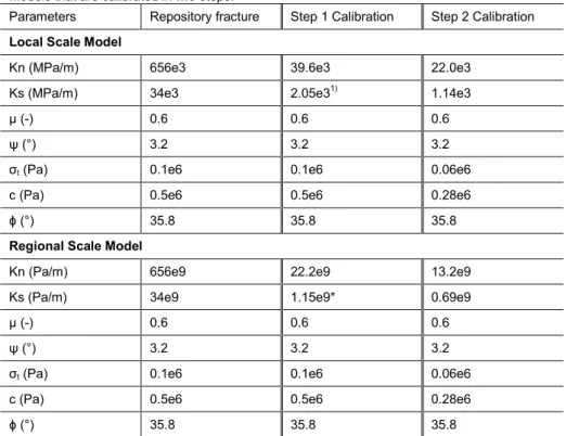
Table 4-5. Mechanical properties of the repository fractures and of smooth joints in the LSM
models that are calibrated in two steps.
Parameters Repository fracture Step 1 Calibration Step 2 Calibration
Local Scale Model
Kn (MPa/m) 656e3 39.6e3 22.0e3 Ks (MPa/m) 34e3 2.05e31) 1.14e3
μ (-) 0.6 0.6 0.6
ψ (°) 3.2 3.2 3.2
σt (Pa) 0.1e6 0.1e6 0.06e6
c (Pa) 0.5e6 0.5e6 0.28e6
ϕ (°) 35.8 35.8 35.8
Regional Scale Model
Kn (Pa/m) 656e9 22.2e9 13.2e9 Ks (Pa/m) 34e9 1.15e9* 0.69e9
μ (-) 0.6 0.6 0.6
ψ (°) 3.2 3.2 3.2
σt (Pa) 0.1e6 0.1e6 0.06e6
c (Pa) 0.5e6 0.5e6 0.28e6
ϕ (°) 35.8 35.8 35.8
4.3. Repository panels
The heat generated from the canisters containing the spent nuclear fuel affects the repository rock and the fractures. In the 2D modelling (Yoon et al. 2016a), the thermal power curve of a full size canister provided by SKB (Fig.4-8, black curve) was modified to meet the two dimensionality of the modelling condition (Fig.4-8, red curve).
Figure 4-8. Thermal power curve of a full size canister according to SKB (black curve)
and the modified one for the PFC2D modelling (red curve).
In the 3D modelling, we use the full size canister thermal power curve (black in Fig. 4-8 and Equation (4-5)). Also, instead of using point heat source as done in the 2D modelling, we used plane heat sources by taking into account the distance between the deposition holes (Px) and the deposition tunnels (Py) as shown in Equation (4-6). The thermal power is then applied to the groups of particles at the locations of the panels.
Equation (4-5)
Equation (4-6)
where, f(t) defines the decay of the heat and the parameters ai and ti are found in
Hökmark et al. (2010).
Heat power assigned to the particles at panel locations is also calibrated. In the 2D modelling, the group of particles at panel locations were treated as a collection of point heat sources and adjusted properly with scaling factors. The scaling factors were introduced in order to take into consideration of the size difference between the particles and the deposition holes (Yoon et al. 2016a).
In the 3D modelling, we take into account the areas of the panels (Fig.4-9a and Table 4-6) and treat the panels as plane heat source similarly to Claesson and Probert (1997) and Probert and Claesson (1997) (Fig.4-9b). Therefore, the thermal
power input we used is in a form of flux with unit of W/m2 and takes into
consideration of full power of the canister (Q = 1700 W), the deposition hole spacing (Px = 6 m) and the deposition tunnel spacing (Py = 40 m). Using Equation (4-6), the panel area (Table 4-6) is multiplied and assigned to the groups of particles acting as heat generating panels. However, due to the fact that the heat source of a
introduced to properly adjust the over-estimated heat power. The reduction factor is calculated from the theoretical panel plane area and the sum of surface area of the particles to which heat power is input. Therefore, the final form of heat input assigned to the particles is given in Equation (4-7):
Equation (4-7)
where, ‘pan’ is geometrical area of the panels listed in Table 4-6.
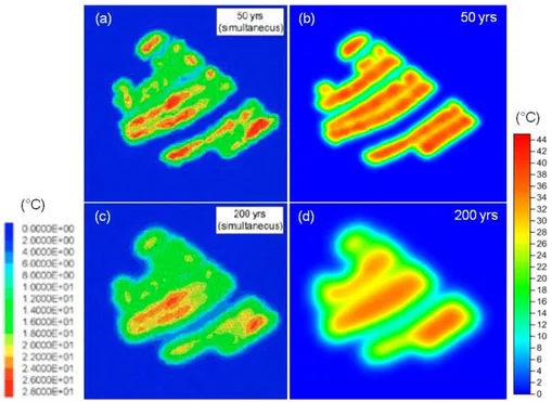
To check if the heat power input is properly calibrated, we perform a heat loading test where the panels are heated simultaneously. In this test the thermal evolution modelling is done in thermal condition only, i.e. without coupling to mechanical analysis. The distribution of the temperature increase at 50 and 200 years after start of heat release are shown in Figure 4-10.
The results we obtained are lower than what is found in Hökmark et al. (2010) where the highest temperature increase at the centre of Panel A is 28 degrees at 50 years and 20 degrees at 200 years.
Table 4-6. Geometrical surface areas of the repository panels (plane heat sources in Fig. 4-9a).
Geometrical area (km2)
Panel A 0.098 Panel B 0.489 Panel C 0.797 Panel D 0.601
Figure 4-9. (a) Repository panels treated as plane heat sources, (b) rectangular plane
heat source model of Claesson and Probert (1997), and (c) particles constructing the panels and treated as volume heat sources.
Figure 4-10. Distribution of rock temperature increase obtained in the PFC3D model (a) 50 years and (b) 200 years at the depth of the repository after start of
Figure 4-11. Distribution of rock temperature increase simulated in 3DEC modelling (left figures) by Hökmark et al. (2010) and in PFC2D modelling (right figures) by Yoon et al. (2016a) at (a) 50 years and (b) 200 years after start of simultaneous panel heating.
4.4. In-situ stress and its evolution during glaciation
Three in-situ stress fields are used for different modelling cases. The reverse faulting
stress field is defined as present day most likely stress model “Stress Model 1, S1” where the maximum horizontal stress (SH) is 40 MPa, the minimum horizontal stress (Sh) is 22 MPa and the vertical stress (Sv) is 13 MPa at the repository depth (Martin 2007). Considering the pore fluid pressure at repository depth, ca. 5 MPa at 500 m, the resulting effective stresses at the repository depth are 35, 17, and 8 MPa, for SH, Sh, and Sv, respectively (Fig.4-12).
Figure 4-12. Depth variation of the in situ stresses (total and effective) of the present day most likely stress model (S1) and the values (dots) at the depth of the repository.
The in-situ stress fields that might evolve during next glacial cycle (time up to 70k
years from present) are based on a reconstruction of the Weichselian glaciations (Lund et al. 2009). Figure 4-13 is used where the glacially induced changes of the
in-situ stress components are read from the curves and added to the in-situ stress
components of present day stress model. Table 4-7 lists the magnitudes of each
in-situ stress components of the stress models: (i) S1: Present day most likely stress
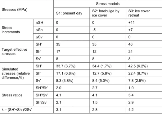
model (Martin 2007); (ii) S2: Glacially induced stress model in relation to forebulge in front of the ice cover (glaciations); (iii) S3: Stress model in relation to the ice cover retreat (deglaciation). Also, the ratios between the effective stresses are presented, which are used for choosing which fault should be activated in the earthquake simulations. In the ice forebulge stress model (S2), the ratio of principal horizontal stresses (SH’/Sh’) becomes larger than that of the present day stress model (S1). This is due to the effect of forebulge induced by the extension of the side of the ice cover, which consequently lowers the minimum horizontal stress (-5 MPa). In such stress condition, some steeply dipping faults are destabilized rather than those gently dipping. Therefore, as it will be discussed in Chapter 6, the large steeply dipping faults are chosen to be activated in the earthquake simulations. In the ice cover retreat stress model (S3), the ratio of horizontal and vertical stresses (SH’/Sv’ and Sh’/Sv’) increase significantly. In such stress condition, the gently dipping faults are more sensitive to destabilization.
We assumed that the increments of the stress components in Figure 4-13 and Table 4-7 are oriented parallel to the principal stress directions of the present day stress model. However, it should be noted that, at the time of deglaciation with remarkably high seismicity, the glacial isostatic processes could lead to a totally new
geodynamic regime; new horizontal stress direction (Mörner 2004). This issue is discussed later.
Figure 4-13. Glacially induced increments of the principal stresses at the repository depth during the Weichselian glaciation (modified after Hökmark et al. 2010).
Table 4-7. In-situ stresses of the stress model at the depth of the repository: Present day most
likely stress model (S1), Glacially induced stress model by ice cover forebulge (S2), Stress model induced by ice cover retreat (S3).
Stresses (MPa)
Stress models
S1: present day S2: forebulge by ice cover S3: ice cover retreat Stress increments ∆SH 0 0 +11 ∆Sh 0 -5 +7 ∆Sv 0 0 0 Target effective stresses SH’ 35 35 46 Sh’ 17 12 24 Sv’ 8 8 8 Simulated stresses (relative difference,%) SH’ 33.7 (3.7%) 34.4 (1.7%) 42.5 (6.2%) Sh’ 17.1 (0.6%) 12.7 (5.8%) 22.4 (6.7%) Sv’ 8.3 (3.8%) 8.4 (5.0%) 7.8 (2.5%) Stress ratios SH’/Sh’ 2.0 2.7 1.9 SH’/Sv’ 4.1 4.1 5.4 Sh’/Sv’ 2.1 1.5 2.9 k = (SH’+Sh’)/2Sv’ 3.1 2.8 4.2
4.5. Dynamic fault rupture
To simulate a fault rupture and an earthquake event, we used the method developed in Yoon et al. (2014, 2016a, 2016b, 2017) where the deformation of the particle contacts (smooth joint contacts) along the earthquake hosting fault is locked during
the initial in-situ stress loading of the model (Step 1 – Locking). In this way, the
strain energy from the loading accumulates at the smooth joints of the deformation zone. The strain energy is then released by instantaneously unlocking the particle contacts (smooth joint contact) of the deformation zone (Step 2 – Unlocking), which results in generation of a seismic wave. The seismic wave then travels through the model, and at the same time attenuates due to the damping in the model (Step 3 – Propagation & Attenuation). We confirmed, in the 2D modelling of a single fault trace dynamic rupture simulation, that a seismic wave is generated from the ruptured fault trace and propagate and attenuates. Also by monitoring the temporal evolution of the stresses at several particles from the ruptured trace, we confirmed that the modelling can also simulate transfer of dynamic and static stresses, similar to a natural earthquake faulting (Belardinelli et al. 1999).
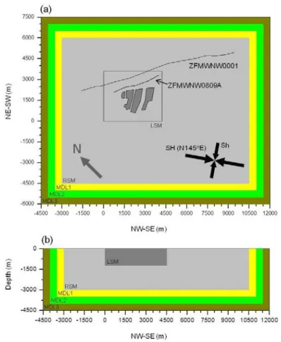
To prevent seismic wave reflection from model boundaries, the following procedure is developed. Figure 4-14 and Figure 4-15 show the Multiple Damped Layers (MDL) located outside the Local Scale Model and the Regional Scale Model, respectively. The MDL concept is developed and implemented in the model in order to simulate energy absorption by the far-field. This measure is taken in order to absorb, as much as possible, the seismic waves both in high and low frequencies that could be reflected back after reaching the model boundaries. Several tests were made to optimize the combination of the relevant parameters, such as, number of MDL, layer thickness, and the damping coefficient of the particles in each MDL that can effectively mitigate the effect of reflecting wave.
Figure 4-14. (a) Top view and (b) side view of the Local Scale Model with Multiple Damped Layers (MDL). Trace of ZFMWNW0809A is shown in the top view for reference.
Figure 4-15. (a) Top view and (b) side view of the Regional Scale Model with Multiple Damped Layers (MDL). Traces of ZFMWNW0001 and ZFMWNW0809A are shown in the top view for reference.
5. Analysis of fracture shear displacement
In this Chapter, we discuss different concepts and methods (continuum model vs. discontinuum model) to analyze fracture shear displacement. Section 5.1 presents the results of FRACOD2D (Shen 2014) analysis and Section 5.2 presents the results of PFC3D modelling. The focus is given to the comparison of shear displacement profiles for different degrees of model complexity considering: fracture geometry (single planar vs. multiple segmented) and material property (elastic medium without fracture propagation vs. inelastic medium with fracture propagation).
5.1. Shear displacement of a single fracture in
continuum model: FRACOD2D analysis
Shear displacement of a fracture embedded in an elastic rock model (Young’s modulus E = 60 GPa and Poisson’s ratio ν = 0.2) is tested using FRACOD2D (Shen 2014). Figure 5-1 shows the model, where on the left side the fracture is planar whereas in the right side the fracture is represented by a collection of smaller joints that are aligned parallel to the main fracture orientation. The left model fracture is referred to as ‘single-planar fracture’, and the right one is referred to as ‘multiple segmented fracture’. The latter is considered to be more natural as rock fractures are usually irregular, non-planar or have other imperfections that prevent shear
movements or have asperities that can be sheared off during slip events.
Figure 5-1. Single fracture represented as (a) a single planar segment and (b) multiple
segments embedded in a continuum model and subjected to 10 MPa and 5 MPa biaxial stresses.
In addition to the geometrical complexity of the fracture, we also tested the fracture shear behaviour under variation of material property: Elastic vs. Inelastic. In the
elastic rock model, the fracture is not allowed to propagate at the tips. This is done
by setting a high fracture toughness (KIC = 2.5 GPa√m and KIIC = 4 GPa√m) to
prevent the fracture from propagating at the tips under the given external loads. In
the inelastic rock model, the fracture is allowed to propagate at the tips by setting
KIC = 2.5 MPa√m and KIIC = 4 MPa√m. Therefore, in total, four cases are simulated
with FRACOD2D.
The first set of results is shown in Figure 5-2 where the shear displacement of a single planar fracture is plotted with respect to normalized distance from the fracture
centre. The red curve shows the absolute displacement of the fracture in the elastic medium. The maximum displacement of 3.96 mm is monitored at the centre. In case of the propagated fracture shown by the blue curve, the maximum displacement at the centre is 4.18 mm, indicating that the maximum displacement increases by 6%. When the normalized displacements are compared (Fig.5-2b), it shows that the displacement near the fracture ends increases due to fracture propagation.
Figure 5-2. FRACOD2D modelling results showing (a) absolute shear displacement and
(b) normalized shear displacement (D/Dmax) vs. normalize distance from the fracture centre (r/R) of the single planar fracture embedded in elastic (red) and inelastic rock (blue).
The second set of results is presented in Figure 5-3, where the shear displacement profiles of the multiple segmented fracture are plotted with respect to the normalized distance from the fracture centre. For comparison, the shear displacement profile of the single planar fracture without fracture propagation (Fig.5-2) is shown in red. In case of the multiple segmented fracture, the normalized displacement profile does not follow the parabolic profile (red curve) but concentrates in the range between a factor 0.6 and 1 of the maximum displacement and uniformly distributed along the entire fracture length. In case when a multiple segmented fracture is embedded in inelastic medium (with fracture propagation) the displacement profile is more widely distributed (Fig.5-3b). It implies that the maximum shear displacement does not always take place at the fracture centre, but can occur near the fracture ends if a rock fracture resembles the multiple segmented fracture.
The reason for larger displacement near the fracture ends can be explained as follows. In case of the single planar fracture, stress concentrates at the fracture tips as shown in Figure 5-4a. However, as the fracture tips are pinned and the
concentration at the extreme ends of the fracture is less than that of the single planar fracture. The result implies that if there are more segments used in representing a fracture, the overall displacement profile could show less displacement at the centre and larger displacement near the fracture ends.
Figure 5-3. FRACOD2D modelling results showing normalized shear displacement of the
segments composing the fracture embedded in (a) elastic rock (no fracture propagation) and (b) inelastic rock (fracture propagation). The right figures show each segment which is colored according to their normalized displacement from the fracture centre.
Figure 5-4. Distribution of maximum principal stress in an elastic rock model containing
The absolute displacements of the segments of the multiple segmented fracture are compared in Figure 5-5. The result shows that the displacement increases generally in case when the fracture segments propagate and interact with other neighbouring fracture segments and form longer continuous fractures (coalescence).
Figure 5-5. Absolute displacement of the segments of the multiple segmented fracture
embedded in the elastic (red) and inelastic (black) models.
5.2. Fracture shear displacement of a fracture in a
discontinuum model: PFC3D analysis
We performed another sets of fracture modelling using PFC3D v4. In the FRACOD2D modelling where the modelled fracture is embedded in a continuum medium, it is seen that the displacement profiles significantly deviate from the parabolic profile if the modelled fracture is represented as a multiple segmented fracture, and shows especially large displacement near the fracture ends. In PFC3D modelling, the fracture is represented by a collection of smooth joints (Mas Ivars et al. 2011), which are embedded in a discontinuum medium represented by a collection of rigid spheres. The spheres are bonded at their contacts with finite stiffness and strength which can fail in different modes (Mode I in tension and Mode II in shear).
In this section we discuss how shear displacement of a fracture represented by a collection of smooth joints (referred to hereafter as a ‘smooth joint fracture’ changes due to the effects of: (i) particle size with respect to a fracture size, (ii) fracture intersection, and (iii) insertion order of the intersecting fractures.
5.2.1. Effect of smooth joint resolution on shear displacement
Three sets of models are generated here to test the effect of particle size relative to the fracture size (i.e. smooth joint resolution for representation of a fracture) on a
fracture shear displacement. The models are 3x6x3 cm3 in size and densely packed
with three different particle size distributions with minimum particle radius of 0.5 mm, 0.75 mm, and 1 mm. Then, an inclined disk fracture is embedded with radius of
smooth joint distributions. As the figures show, due to different particle size
distribution, the patterns of smooth joint distributions are different. It is seen that the finer the particle resolution, the smaller the size of the smooth joints, and the narrower the width of the smooth joint clusters in the direction normal to the fracture plane.
Figure 5-6. Densely packed particle assembly with different particle size distribution
(minimum particle radius of (a) 0.5 mm, (b) 0.75 mm, (c) 1 mm) and with an inclined fracture embedded at the centre. The bottom figures show the side views.
The models are then loaded triaxially with 10 MPa vertical stress (σzz) and 5 MPa
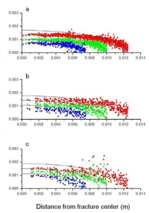
lateral stress (σxx=σyy). Figure 5-7 shows the shear displacement of the smooth joints
with respect to their distance from the fracture centre. The numerical results show that, in general, the smooth joint shear displacement is large at the fracture centre and tapers towards the tips. The solid lines plotted in the figure are the analytically determined shear displacement distribution of a planar fracture with identical radius using the following analytical solution (Segedin 1951):
Eqn. (5-1)
where, G is the shear modulus of the rock model, v is Poisson’s ratio and ∆τ is the
applied shear stress on a fracture, a is the fracture radius, and r is the distance of the
occurrence point of the shear displacement from the fracture centre. The elastic
constants E, G, and v of the models in Figure 5-6 are determined from uniaxial
compression tests. The analytically determined shear displacement shows parabolic profile with maximum at the fracture centre and tapering toward the fracture tips. The analytical solution, Eqn. (5-1), expresses the shear displacement distribution of a perfectly planar and frictionless fracture embedded in an elastic medium.
Therefore, the energy given by the external loading is spent mostly on displacing the fracture and therefore it results in the largest displacement at the fracture centre.
However, in the PFC3D models, the fracture is not planar and the bonded particle assembly also deforms by the external loading. The energy provided by the external loading is then partitioned by the slip of the smooth joints.
The numerical results show that the displacement profile is rough and the degree of fluctuation becomes more significant with increasing particle size, i.e. in the coarser resolution model (Fig.5-7c). Moreover, the shear displacement profile of the largest fracture (red profile) is generally higher for the case of a coarse particle resolution model. The reason for such large shear displacement and high irregularity is due to the gap between the smooth joints. The gap between the smooth joints (inter-segment area in 2D or volume in 3D) is larger as the particle resolution becomes coarser. And as the gap between the smooth joints becomes larger, there are more rigid particles in the area between the smooth joints, which results in higher stress concentration. Higher concentration of stress at the inter-segment volume results in large shear displacements of the segments (smooth joints) near the stress
concentration.
Figure 5-7. Shear displacement of the smooth joints of the fractures embedded in (a) fine
resolution, (b) intermediate resolution, and (c) coarse resolution models. The solid lines represent analytically determined shear displacement of a planar fracture with same size.
intersecting other fractures. It was found that such displacement spikes at the intersection locations occur due to presence of particles that become detached from the surrounding particles, therefore so called “rattler particles”. A numerical algorithm for detecting and deleting rattler particles is developed and tested in a 2D model with five intersecting fractures as shown in Figure 5-8a. The results show that the displacement spikes (Fig.5-8b) disappear after eliminating the rattler particles from the model (Fig.5-8c), and become similar to the results of FRACOD2D modelling (Fig.5-8d).
Figure 5-8. (a) 2D model with five intersecting fractures and loaded 10 MPa axially and 2
MPa laterally, (b) shear displacement distributions of five intersecting fractures before deleting and (c) after deleting the rattler particles, and (d) shear displacement distributions obtained from FRACOD2D modelling (Yoon et al. 2016a).
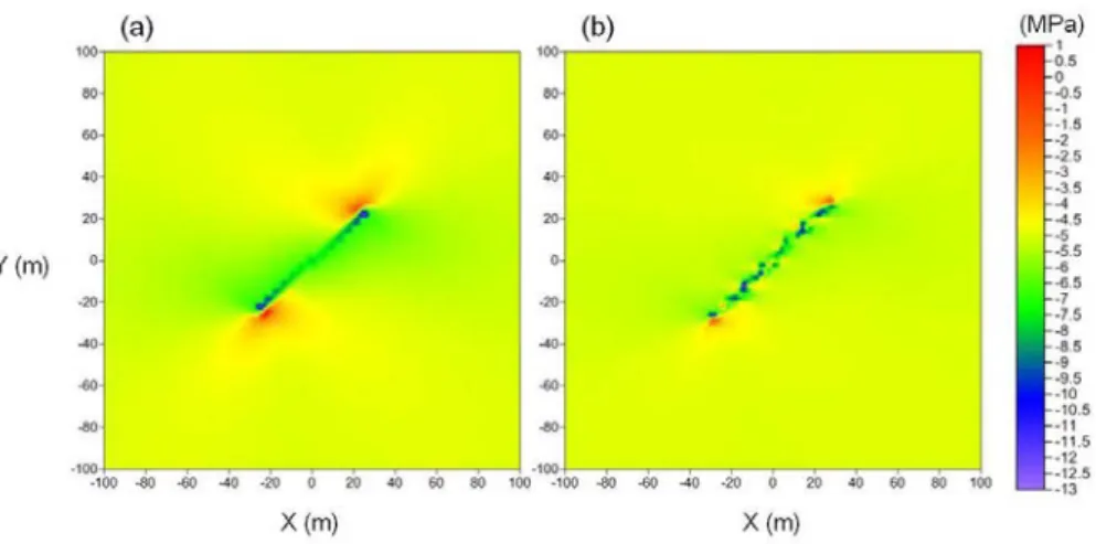
We also applied the algorithm to the 3D PFC model with five intersecting fractures.
The 3D model is shown in Figure 5-9 with axial stress (σzz) of 10 MPa and lateral
stress (σxx=σyy) of 2 MPa. The shear displacement distributions of the fractures are
shown in Figure 5-10 with respect to the distance of the smooth joint from the fracture centre. The results show that there are several smooth joints with
significantly large shear displacement, but these shear displacements are eliminated by deleting the rattler particles. However, there still exist several smooth joints, especially at fracture 1 and fracture 3, showing sharp increase and drop of the displacements.
Figure 5-9. (a) 3D model with embedded five intersecting fractures and subject to triaxial loading and (b) the equivalent 2D model (Yoon et al. 2016a).
Mean shear displacements are calculated for the fractures and presented in Table 5-1. The values in the left column are the mean displacement before deleting the rattler particles (Fig.5-10, left figures), and those in the right column are the mean displacement after deleting the rattler particles (Fig.5-10, right figures). The results show that the relative differences are between 2 and 10%.
Also, median shear displacements are calculated for the fractures and presented in Table 5-2. The values in the left column are the median displacement before deleting the rattler particles (Fig.5-10, left figures), and those in the right column are the mean displacement after deleting the rattler particles (Fig.5-10, right figures). The results show that the relative differences are negligible.
The results demonstrate that median value of the smooth joint shear displacements provides robustness for determination of a representative shear displacement of fractures that are made up of many smooth joints and intersected by neighboring fractures. This result supports our decision for use of median over mean, which is discussed later in Section 5.4.
Table 5-1. Mean shear displacements of the fracture: before deleting the rattler particles (left
column) and after deleting the rattler particles (right column).
Mean shear displacement (cm) Relative difference (%) Before After Fracture 1 5.10 4.91 3.7 Fracture 2 2.51 2.52 0.4 Fracture 3 1.17 1.09 6.8 Fracture 4 2.36 2.33 1.3 Fracture 5 1.38 1.38 0.0
Figure 5-10. Shear displacement of the smooth joints of the 3D fractures (a) before and (b) after eliminating the rattler particles.
Table 5-2. Median shear displacements of the fracture: before deleting the rattler particles (left
column) and after deleting the rattler particles (right column).
Median shear displacement (cm) Relative difference (%) Before After Fracture 1 5.10 5.01 1.8 Fracture 2 2.31 2.32 0.4 Fracture 3 0.83 0.83 0.0 Fracture 4 2.48 2.47 0.4 Fracture 5 1.38 1.38 0.0