(HS-IDA-EA-01-104)
Henrik Grimm (a98hengr@student.his.se)
Institutionen för datavetenskap Högskolan i Skövde, Box 408
Submitted by Henrik Grimm to Högskolan Skövde as a dissertation for the degree of B.Sc., in the Department of Computer Science.
2001-06-18
I certify that all material in this dissertation which is not my own work has been identified and that no material is included for which a degree has previously been conferred on me.
Henrik Grimm (a98hengr@student.his.se)
Abstract
Simulation means running a model of a system with suitable input and observing the corresponding output. Real-time environment simulation is a special kind of simulation used to simulate a control system’s environment in real-time. This is done to test the control system before it is used in its real environment. In this project, computer simulation of a certain kind of environments, called track-based systems, is studied and a general model for track-based systems is developed. In this model, track layouts are represented by graphs, which is a flexible and extensible representation and a method for visualizing these layouts is presented. The model also includes representation of switches, sensors, and trains. In addition, a configurable prototype simulator is designed and implemented for a model railroad system. The experience gained in this project is documented in the report and is presented as guidelines for developing simulators for track-based systems.
Keywords: Environment Simulation, Track-Based Systems, Real-Time Systems, Modeling, Testing.
1
Introduction ... 1
2
Background... 2
2.1 Real-time systems ... 2
2.1.1 Environments and control systems... 2
2.1.2 Real-time facilities ... 4
2.2 Modeling and Simulation ... 5
2.2.1 Types of simulations ... 7
2.2.2 Real-time environment simulation... 9
2.2.3 Verification and validation ... 11
2.3 A digitally controlled model railroad system ... 12
3
Problem definition ... 15
3.1 Motivation... 15
3.2 Track-based systems... 15
3.3 Aims and objectives ... 16
3.3.1 Objective 1: Modeling track-based systems ... 16
3.3.2 Objective 2: Implement prototype simulator... 16
3.3.3 Objective 3: Extraction of design guidelines... 18
3.4 Scientific approach and expected results... 18
4
Model of track-based systems ... 20
4.1 Track layout ... 20
4.1.1 Lengths of track pieces ... 22
4.1.2 Positions on track ... 22
4.1.3 Visualization ... 24
4.2 Dynamic objects... 24
4.2.1 Train movement ... 24
4.2.2 Detecting critical states... 26
4.2.3 Switches... 28
4.2.4 Sensors... 29
5
Design and implementation of prototype simulator ... 30
5.1 Architectural design ... 30
5.2 Simulator interface ... 31
5.3 Implementation of model... 33
5.3.3 Static nodes and switches ... 35
5.3.4 Sensors and collision detection... 36
5.4 Visualization of the simulated environment ... 36
5.5 Configurability ... 37
6
Conclusions ... 39
6.1 Summary... 39 6.2 Related work ... 40 6.3 Future work... 42 6.3.1 Validation of simulator... 426.3.2 Further development of prototype... 43
6.3.3 Distributed simulation ... 43
Acknowledgements ... 45
1 Introduction
Simulation means running a model of a system with suitable inputs and observing the corresponding output (Bratley, et al., 1987). Simulations can be performed in a number of ways. The type that is of interest for this project is computer simulation, where a computer program is used to simulate another system. These programs are called simulators.
Simulation can be performed for a number of reasons. One is to analyze a system to gain further insight into its dynamics. By feeding input to the simulation and observing its output, the operator can test conditions that are difficult or unsafe to test on the real system, e.g. a core meltdown in a nuclear power station. Another type of simulation is used to train users or operators in a safe way, e.g. pilots training in flight simulators. The type that is of interest for this project is environment simulation, which is used to test a control system before it is connected to its real environment. There are many reasons for using an environment simulator before the control system is used with the real environment; it is often cheaper and safer and the operator has more control over the environment simulator (e.g. to test conditions that rarely happen in the real environment). An environment simulator must often imitate the temporal behavior as well as the functional behavior of the modeled system, which puts real-time requirements on the simulator. This makes environment simulators difficult and hence expensive to develop.
According to Bratley, et al. (1987), simulation is widely applied in engineering, in business, and in the physical and social sciences. One domain where environment simulation is of great importance is in the development of safety critical control systems. There exists few works covering the development of such simulators, mainly because it is hard to draw general conclusions for all types of systems. However, many similar simulation problems may arise in a specific sub-domain. This work covers one specific sub-domain, called track-based systems. Track-based systems are systems with the same general characteristics as railroad systems, i.e. vehicles that follow a track. This work aims to investigate methods for modeling and simulating track-based systems with real-time constraints.
Chapter 2 contains the background material for this project, covering real-time systems, environment and control systems, modeling and simulation, and a description of the model railroad system. In Chapter 3, the problem is motivated and track-based systems are further defined. This is followed by stating the aim and objectives and the expected result for this project. Chapter 4 describes a model developed in this project. In Chapter 5, the design and implementation of a prototype simulator is described. Finally, Chapter 6 presents a summary of the report, work that is related to this project, and suggestions for future work.
2 Background
This chapter gives some background and definitions of the terms that are used throughout this report. In Section 2.1, relevant issues on real-time systems and their environments are described. Section 2.2 explains the concept of models and how models can be used for simulation. In Section 2.2.1, some different types of simulation are described. Real-time environment simulation is explained in Section 2.2.2, followed by a description of verification and validation of simulators in Section 2.2.3. In Section 2.3, the model railroad, which is used for a case study in this project, is described.
2.1 Real-time
systems
According to Ingels (1985, p. 31), a system can be defined as:
a device or process which accepts one or more inputs and from them generates one or more outputs.
In real-time systems the time at which outputs are produced are important, unlike in traditional computer systems, which are built only for information processing. A real-time system must provide services in two dimensions: the functional dimension and the temporal dimension (Schütz, 1993). Not only does output have to be correct, but it must also be provided in a timely manner. This makes real-time systems harder to implement and test than non-time systems. There are many definitions of real-time systems, e.g. (Schütz, 1993, p. 2):
A real-time system is a system whose correctness depends not only on the logical result(s) of a computation, but also on the time at which the results are produced.
A real-time system can also be defined as a system that changes its state as a function of (real) time (Kopetz & Verissimo, 1993).
2.1.1 Environments and control systems
Real-time systems often interact with physical equipment in the real world, called the system’s environment. This type of real-time system is called a control system, because its purpose is often to control something in the environment, e.g. a thermostat controlling the temperature in a room. The control system interacts with the environment through sensors and actuators, which are collectively called the
instrumentation interface (Kopetz & Verissimo, 1993). A sensor reads the state of
something in the environment and presents the percept (also called sensor reading) to the control system. Examples of sensors are temperature sensors, light sensors, and pressure sensors. While receiving percepts, the control system can act upon the environment by sending actions to the environment’s actuators. An actuator is something in the environment that can be used by a control system to affect the state of the environment. Examples of actuators are valves and conveyor belts. Figure 1
E n v iro n m e n t Ac tuato r s S ens o rs Co ntro l s ys te m ac tio ns pe rc epts Instrum e nt atio n inter fac e
Figure 1: Relationship between a control system and its environment.
In Figure 1, the control system is drawn outside the environment for illustration purposes. In real environments, the control system is often part of the environment. This type of control system is called an embedded system. The terms real-time and embedded are often used interchangeably.
When the control system acts on its environment, the state of the environment probably changes. In most real-world environments this is further complicated because the state of the environment is changed by other events in the environment, even if no actions are issued by the control system. This is called a dynamic environment (Russel & Norvig, 1995). Because of this, the control system must have real-time facilities in order to control processes in the environment with respect to time. Real-time facilities are covered in Section 2.1.2.
Figure 2 shows an example of a control system and its environment, taken from Burns and Wellings (1997). The environment is a pipe where some liquid flows. The purpose of the control system is to ensure an even flow through this pipe. The instrumentation interface consists of one sensor and one actuator. The sensor is a flow meter that measures the flow and the actuator is a valve that controls the flow. When receiving a flow reading, the control system must respond in a specified time if the equipment at the receiving end of the pipe is not to become overloaded.
C o ntro l s ys tem
V alve angle F lo w read ing F lo w m eter V alve
Figure 2: A fluid control system (after Burns & Wellings, 1997, p. 4).
As this example illustrates, the duration between a percept from the environment and the response to the environment is time constrained. The sequence of all
communication and processing steps between such a percept and response is called a
real-time (RT) transaction (Kopetz & Verissimo, 1993). A real-time transaction must
deliver the correct result at the intended point in time. Otherwise, the system has failed.
According to Burns and Wellings (1997), real-time systems are often distinguished as either hard or soft. In a hard real-time system, it is absolutely imperative that responses occur within the specified deadline. If a deadline is missed, then the system fails, which can have catastrophic consequences. Soft real-time systems are those where response times are important, but the system still functions correctly if deadlines are occasionally missed. Soft real-time systems can further be distinguished from interactive real-time systems, which have no explicit deadlines but strive for “adequate response times”. Many systems have both hard and soft real-time subsystems and some services may have both a hard and a soft deadline.
Real environments are often very complex and the sensors do not give access to the complete state of the environment. This is called an inaccessible environment (Russel & Norvig, 1995). To cope with this, the control system often maintains an internal model of the environment. This internal model is generally an abstraction (simplification) of the real environment. When a percept is received, the internal model is updated to keep it synchronized with the real environment. Depending on the state of the internal model, the control system makes decisions on how to use the actuators in the real environment.
According to Russel and Norvig (1995), an environment is deterministic if the next state of the environment is completely determined by the current state and the actions selected. However, most real environments are so complex that they must be treated as non-deterministic for practical purposes.
2.1.2 Real-time facilities
In order for a system to be able to meet response times, it must have access to real-time facilities. According to Burns and Wellings (1997, p. 13), real-real-time facilities should enable the programmer to:
• Specify times at which actions are to be performed. • Specify times at which actions are to be completed.
• Respond to situations where all the timing requirements cannot be met.
• Respond to situations where the timing requirements are changed dynamically.
In order to achieve this, the control system must have access to some type of clock, measuring the passage of time. According to Burns and Wellings (1997, p. 359), this can be done in two distinct ways:
• By giving the control system direct access to the environment’s time frame. • By using an internal hardware clock that approximates the passage of time in
Wellings, 1997). When delaying processes there is a difference between the time that is specified and the actual time of wakeup. This difference is called the local drift and cannot be eliminated. It is dependent on many things, e.g. the granularity of the clock, the underlying operating system, and the priority of the process. If a process is delayed at regular intervals, then the local drifts can superimpose. This is called the
cumulative drift and it can be eliminated by delaying to absolute points in time instead
of delaying for relative periods (Burns & Wellings, 1997).
Further, a real-time system must be able to recognize, and act upon, the non-occurrence of some external event (Burns & Wellings, 1997). A timeout is a restriction on the time a process is prepared to wait for a communication.
2.2 Modeling and Simulation
A model is an abstract description of a system that is formulated in some adequate and convenient notation, either formally or informally (Schütz, 1993). The system being modeled is called the original system in this report. The original system is often a real world system, but can be any type of system. A model is often used to gain further insight into the relationships among various components or to predict performance under some new condition being considered (Law & Kelton, 1991).
One system is a perfect model of another if the former produces exactly the same output as the latter under the same inputs (Bratley, et al., 1987). Real world systems are often very complex and it is therefore virtually impossible to create a perfect model of these systems. Some details of the original system must be abstracted from, while properties that are more important are analyzed. It is generally not necessary to have a one-to-one correspondence between each element of the original system and each element of the model (Law & Kelton, 1991). The challenge is to find a model that is sufficiently precise to be useful for its intended application, yet simple enough to understand and finish in desired time. According to Bratley, et al. (1987), modeling a real system is largely ad hoc. It must always be checked if the model reflects the features of the original system that are important to the application in mind.
According to van den Bosch and van der Klauw (1994), an important decision in deriving models is the selection of the system boundary that determines which parts of the original system that are taken into account. This selection can be critical. If it is too wide, then it is difficult to estimate the parameters of the model and it may be difficult or impossible to use it. If it is too narrow, then not all relevant aspects of the original system are incorporated in the model, which leads to unsatisfactory results. That is, if too many factors in the original system are abstracted from, then the simulation is not a sufficiently precise approximation of the original system. However, many factors in the original system may be very difficult and time-consuming to model and it may be possible to get a model that is sufficiently precise without them.
A state of a system is the collection of variables necessary to describe the system at a particular point in time (Law & Kelton, 1991). When building a model, each state must contain enough information about the history so that, given the current state, the past is irrelevant for predicting all future behavior that is of interest to the application (Bratley, et al., 1987). The state changes according to one-step probabilities that depend only on the current state, events, and the passage of time. Several of the
abstractions made in going from the original system to a model have the effect of reducing the number of states, which makes the model more tractable (Bratley, et al., 1987).
When there is something about the system’s behavior that is poorly understood or difficult to model, assumptions about the causes must be made (Ingels, 1985). These assumptions must be clearly stated so that if the model differs too much from the original system, these assumptions can be refined and retested.
According to van den Bosch and van der Klauw (1994), two approaches to modeling are white-box modeling and black-box modeling. White-box modeling assumes complete knowledge of the original system and the model is derived by using physical knowledge and assuming ideal components. In black-box modeling, no knowledge of the process is used and all parameters must be estimated from measurements of inputs and outputs. A third approach, gray-box modeling, is used when physical laws can be used to arrive at a model, but not all parameters in the model are known. In this case, the physical model is used, but the parameters must be obtained in another way (van den Bosch & van der Klauw, 1994).
After creating the model, the second step is to “implement” the abstract model in order to get a model, which can be used for the desired application (Schütz, 1993). This model can be one of several types, e.g. analytical models (e.g. a set of equations), physical models (e.g. a flight simulator), or computer models. Manipulating an analytical model is not considered simulation, but in all other cases, experimenting with the model is termed simulation. According to Bratley, et al. (1987, p. 2), simulation means, “driving the model with certain (typically random) inputs and observing the corresponding outputs”.
The type of simulation that is of interest for this project is computer simulation, where a computer program is used to simulate a system. These programs are often called
simulators and are used to imitate the original system. A simulator can be used to test
both normal and abnormal behaviors of the original system. The steps involved when creating a simulator are illustrated in Figure 3.
O riginal
s yste m F o rm ulatio n M o de l Im p le m e n ta tion S im ulato r
Figure 3: The steps involved when creating a simulator.
Some advantages with simulation are (Law & Kelton, 1991, p. 115):
• Most real-world systems cannot be evaluated analytically. A simulation is
often the only investigation possible.
• Simulation can be used to estimate the performance of an existing system
under some conditions.
• Experiments with simulation can be executed both in compressed time (e.g.
for economic models) and in expanded time (e.g. for quantum processes). Drawbacks with simulation are that it is often difficult to create a model that has sufficient precision for the intended application and they are often expensive and time-consuming to develop (Law & Kelton, 1991).
2.2.1 Types of simulations
According to van den Bosch and van der Klauw (1994), there are several types of models used to describe systems. These can be divided into mathematical and non-mathematical models. Examples of non-non-mathematical models are scale models (physical models) and verbal models. Mathematical models can further be divided in static and dynamic models. A static model is a representation of a system at a particular time, or one where time plays no role (Law & Kelton, 1991). A dynamic model represents a system as it evolves over time. In this section, three types of simulation of dynamic systems are described: discrete event simulation, continuous simulation, and combined discrete-continuous simulation.
Because these models are dynamic, they must keep track of time as the simulation proceeds. This is called the simulation time. Generally, there does not need to be any relationship between simulation time and real time. An exception to this is real-time simulation, where these must be synchronized. Real-time simulation is covered in Section 2.2.2.
2.2.1.1 Discrete-event simulation
In discrete-event models, the simulation time is advanced in discrete steps, called
events. An event is defined as an instantaneous occurrence that may change the state
of the system (Law & Kelton, 1991). In between two events, the state of the system is retained, i.e., the state can only change when an event occurs. An event can happen due to external events or due some timetable, which can be produced as a result of internal activities (van den Bosch & van der Klauw, 1994). The variable in the simulation model that gives the current value of simulation time is called the
simulation clock (Law & Kelton, 1991).
There are two principal approaches for discrete-event simulation: asynchronous and synchronous simulation. The difference between these is how the simulation clock is advanced.
In asynchronous discrete-event simulation, the approach used to advance the clock is called next-event time advance (Law & Kelton, 1991). With this approach, the clock is initialized to zero and the times of occurrence of future events are scheduled in an event list. For each iteration, the simulation clock is updated to the earliest of these future events in the event list and the system is updated to account for the fact that the event has occurred. An example of this is illustrated in Figure 4. An event can in turn schedule new events that will occur in the future, which are added to the event list.
Figure 4: Example of an asynchronous discrete-event simulation where e1, e2, and e3 are events. For
each iteration, the simulation clock is advanced to the next event.
In synchronous discrete-event simulation, the approach used to advance the clock is called fixed-increment time advance (Law & Kelton, 1991). A synchronous discrete-event model is a special type of an asynchronous discrete-discrete-event model, where discrete-events happen at fixed, regular intervals (Bratley, et al., 1987). Instead of simulating events when they occur, the model is advanced at regular intervals: 0, ∆t, 2∆t, etc., where ∆t is some constant time interval. Events which occur between these fixed time steps are postponed to the next regular time step (Bratley, et al., 1987). That is, an event that occurs at time a∆t + b, where a is some integer and b < ∆t, are postponed to happen at time (a + 1)∆t. An example of this is illustrated in Figure 5.
Figure 5: Example of a synchronous discrete-event simulation. Event e1 is postponed to happen at time
∆t and events e2 and e3 are postponed to happen at time 3∆t.
According to Bratley, et al. (1987), this method has a number of drawbacks, but one major advantage. First, these models are difficult to program, because events that occur between the same time steps usually lead to complicated problems of priority and sequencing (to decide in what order the events should be executed). Second, to obtain a sufficiently accurate estimate it may be necessary that ∆t is very small. This can lead to many “unnecessary” time steps where no events are executed, which can make the simulation inefficient. Another disadvantage is the error introduced by delaying events to the end of the interval in which they occur (Law & Kelton, 1991). According to Bratley, et al. (1987), the major advantage with synchronous simulation is that it is relatively easy to implement so called wait-until statements, where a certain event should occur at the time a particular condition is satisfied (which may include a reference to simulated time). This may be difficult or impossible to implement correctly in an asynchronous model, because conditions can only be evaluated when events occurs. If a condition becomes true it is not known until the next event occurs or maybe not at all, because by then the condition may be false again. When using synchronous models, this can be solved by scanning all conditions for every time step and execute the corresponding event if a condition becomes true (Bratley, et al., 1987).
2.2.1.2 Continuous simulation
Continuous simulation is used to solve models with continuously changing states
(Bratley, et al., 1987). This type of models is used when state variables change continuously with respect to time. They are often composed of a number of differential equations that give relationships for the rates of change of the state variables with respect to time (Law & Kelton, 1991). The goal is to calculate the state of a system at some time in the future, given an initial configuration.
An example of this type of model is the well-known relation d = vt, where v is the velocity of some object, t is the time spent moving with this velocity, and d is the distance moved during this time. The moved distance (d) is continuously changing with respect to time (t).
2.2.1.3 Combined discrete-continuous simulation
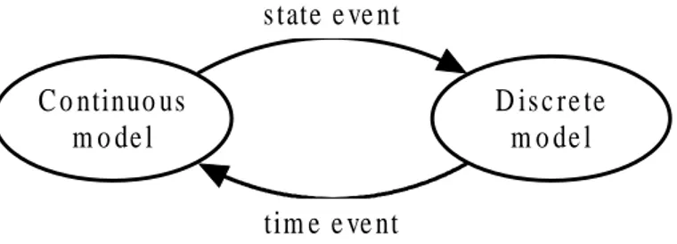
According to Law and Kelton (1991), some systems are neither completely discrete nor completely continuous. This calls for a model with aspects of both discrete-event simulation and continuous simulation, resulting in combined discrete-continuous
simulation. The interactions between a discrete-event simulation and a continuous
simulation are realized with state events and time events (van den Bosch & van der Klauw, 1994). A time event is a discrete event that may cause a discrete change in the value of a continuous state variable. A state event is when a continuous variable in the continuous model is achieving a threshold value, which causes a discrete event to be scheduled. These interactions are illustrated in Figure 6.
C o ntinuo us m o de l D is c re te m o de l s tate e ve nt tim e e ve nt
Figure 6: Interaction between continuous and discrete models (after van den Bosch & van der Klauw,
1994, p. 11).
The following is an example of this type of system, after van den Bosch and van der Klauw (1994, p. 13): Many gas-fired central heating units are equipped with a gas valve that can only be open or closed (no intermediate value). If this unit is controlled by a room thermostat, then the valve is opened when the temperature drops below some threshold value and it is closed when the temperature becomes larger than another threshold value. In this system, the temperature is continuous with respect to time while the valve actions are discrete. When the temperature achieves some threshold value, a state event is issued to either open or close the valve.
2.2.2 Real-time environment simulation
For general simulators there does not have to be a relationship between simulation time and the original system’s timeframe. However, if the original system is a real-time system and it is not a closed system (i.e. the system interacts with some external
system), then the simulation time has to be kept synchronous to the system time of the original system (Schütz, 1993). This type of simulator is a real-time system in its own right and is called a real-time simulator. A real-time simulator must reproduce the temporal behavior of the original system as well as the functional behavior.
An environment simulator is a special kind of simulator that is used to simulate a control system’s (physical) environment. An environment simulator must often be executed in real-time, because the environment interacts with another system (the control system), which also is a real-time system. It should be transparent to the control system whether it interacts with the simulator or the original environment. This is achieved by having the same instrumentation interface (sensors and actuators) to the environment simulator as to the original environment. Figure 7 illustrates the relationship between a control system and its environment simulator. Compared to Figure 1, the original environment is replaced with the environment simulator. For the control system, there is no difference, except that the simulator may respond differently from the original environment due to abstractions and approximations in the model. C o ntro l s ys te m ac tio ns pe rc e pts E nviro nm e nt s im ulato r Ins tr um e ntatio n inte r fac e
Figure 7: Relationship between a control system and its environment simulator (cf. Figure 1).
According to Bergström (1996), environment simulation is often used for another purpose than traditional (non-environment) simulation. While traditional simulation is used to analyze and gain further insight into the original system, an environment simulator is often built for testing a control system before it is used in the original environment. There are several reasons for using an environment simulator for testing purposes (Schütz, 1993):
• It is often cheaper to test a control system with an environment simulator than
with the original environment (e.g. the control system in a space shuttle).
• With an environment simulator, behaviors that are hard or unsafe to test in the
original environment can safely be tested (e.g. an emergency landing in a flight simulator).
• Often, the tester has more control over the simulator than the original
environment. Therefore, test execution is faster, easier, and more flexible. Events that rarely happen in the original environment can be tested just as easily as normal events. This is good for verifying the fault-tolerance of control systems.
• Sometimes the original environment is not yet available. A simulator can be
used to test the control system before the “original” environment exists.
• A simulator can give information about the internal state of the environment
Another purpose of an environment simulator is for user or operator training (Schütz, 1993). One example of this is flight simulators, which are built exclusively for training purposes.
In order to achieve these goals the behavior of the simulator must match that of the original system as close as possible. The better they match the higher the precision of the simulator. How the precision can be measured is covered in Section 2.2.3.
A possible disadvantage of using a simulator compared to using the original environment is that the simulator is a black box, only taking inputs and returning outputs without giving any feedback of its internal state. Often it is desired to get some feedback from the environment when testing and debugging a control system, because it is easier to interpret what really happens. In a simulator, this can be realized by giving the simulator some means of visualizing the simulated environment. This visualization can be everything from simple textual output showing the state of some internal variables to a full-blown graphical representation of the environment. Either way, if the simulation is performed in real-time, then the visualization must also be carried out in real-time; because the information is less valuable the longer it is delayed before being visualized.
Further, it is also desirable that the simulator has a user interface, where the simulated environment can be controlled, both before and during execution. If the simulator shows a graphical visualization of the environment, then this can be integrated with the controlling interface to create a graphical user interface where the user can interact with simulated objects to change their states.
2.2.3 Verification and validation
To check if a model and the program implementing it represent the real system can be checked in two stages (Bratley, et al., 1987). Verification is the process of making sure that the implementation of the model is consistent with the model and free of bugs. That is, verification checks the translation of the model into a correctly working program. Validation is the process of making sure that the simulation model is a sufficiently close approximation to the original system for the intended application. If this is the case, then the model is valid for its intended application (Law & Kelton, 1991). These steps are illustrated in Figure 8.
O r igin al s y s te m F o r m ulatio n M o d e l Im p le m e nta tion S im u lato r
Validatio n Ve r if ic atio n
Figure 8: Conceptual illustration of validation and verification.
According to Law and Kelton (1991), one of the most difficult problems when building a model is that of validation. It is often difficult to know if a model is good until the simulator is implemented and tested. If the simulator produces unacceptable output compared with the original system, it is not always clear if this is due to errors in the implementation or due to abstractions and approximations in the model.
The higher confidence one have that the implementation contains no faults, the more likely it is that any differences between the original system and the simulator are due to approximations in the model. It is therefore important that the simulator is designed and implemented in a sound and structured way to ease the verification. Verification of a simulator is not different from verification of any other type of computer program; all standard tools for debugging computer software apply to debugging simulators (Bratley, et al., 1987).
2.3 A digitally controlled model railroad system
In this work, a model railroad system is used for a case study to evaluate the model and design guidelines that are presented in this report. The railroad is digitally controlled, which means it can be controlled from a computer and it is possible to develop programs that interact with the railroad. The interface system of the railroad communicates with the computer over a serial link. According to the definitions in Section 2.1.1, the railroad is the environment and the computer program is the control system as illustrated in Figure 9.
Se rial link
C o ntro l s ys te m E nviro nm e nt
M odel railroad
Figure 9: The computer program controls the model railroad over a serial link.
On the track, there can be a number of vehicles. A vehicle can be either an engine or a car. These vehicles can be coupled to each other to form trains. The engines can run both in the forward direction and in the reverse direction and there are 15 levels of speed (numbered 0 to 14, where 0 is non-moving and 14 is the fastest speed). Some of the engines have a special function that can be activated. Examples of this are lights in front of the engine and decoupling functions.
At some points on the track, there are switches where the trains either go straight or turn into another track depending on the state of the switch. All switches are in one of two states: straight or turning. This is illustrated in Figure 10.
Figure 10: A switch is in one of two states: straight or turning.
Some parts of the track are called decoupling rails, which are used to decouple engines and cars from each other. Some trains also have a decoupling function, which
On the track, there are a number of sensors of different types. A sensor is activated when a train passes it and deactivated otherwise. There are three types of sensors: direction sensors, optical sensors, and position sensors. The main difference between these is that when a direction sensor is activated, it recognizes which direction the train is heading in, while the other two types do not give this information. The control system gets the status of sensors by polling, i.e. it sends a request to the railroad and gets the status of all sensors in response.
On the track, there are some light signals, which can be either turned on or turned off. They have no effect on the rest of the railroad, but can be handy when testing and debugging an application for showing different states and conditions.
The railroad is a typical real-time environment. It contains a number of actuators and sensors and the environment is dynamic, i.e. the state changes by the passage of time. For example, when a train is started, it runs until it is stopped by the user or runs into something (e.g. another train).
Here follows a summary of the actuators and sensors (and their possible states): Actuators:
• Speed of engines (0-14)
• Direction of engines (forward/reverse) • Engine functions (on/off)
• Railroad switches (straight/turning) • Decoupling rails (activated/deactivated) • Light-signals (on/off)
Sensors:
• Direction sensors (activated/deactivated, right/left) • Optical sensors (activated/deactivated)
• Positions sensors (activated/deactivated)
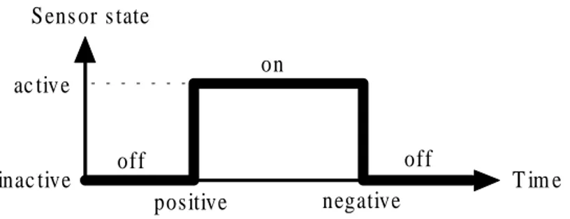
A train control program has been developed at the University of Skövde (Nilsson, 2001). This program handles the low-level communication with the railroad to make it easier to develop applications for it. To get information about a sensor being activated, a process sends a request to the train control program. The train control program polls the hardware registers at regular intervals and sends information of changed sensor readings to processes that have explicitly requested such information. A request can be specified to be once (the request is automatically removed after the matched request) or repeated (sensor notifications are sent until the request is explicitly revoked). A request is specified for one sensor and in one of four different modes: “on”, “off”, “positive”, or “negative”. In “positive” mode, the notification is sent on the transition between the active and inactive sensor states. In “on” mode, the notification is sent if the sensor is active when the signal is requested (this is useful to detect if a train is placed on a sensor when the request is sent). The other two modes: “negative” and “off”, are similar for the active to inactive transition and inactive state respectively. These modes are illustrated in Figure 11.
ac tiv e inac tive positive negative on off off Sens or s tate T im e
Figure 11: Sensor information can be requested in one of four different modes: “on”, “off”, “positive”,
3 Problem definition
This section introduces the problem that is studied in this project. First the motivation is given in Section 3.1, where it is explained why this is a relevant and interesting problem. In Section 3.2 track-based systems is defined. This is followed by stating the aim and objectives in Section 3.3. The objectives are further described in Sections 3.3.1 to 3.3.3. Section 3.4 describes the expected results of this work and summarizes the chapter.
3.1 Motivation
As mentioned earlier, creating a model of a real system is largely ad hoc. Few general guidelines exist for creating models and simulators are often developed on a project-by-project basis (Bergström, 1996). A reason for this is that the systems that are modeled range over a wide area of types and hence requires different approaches, e.g. communication networks (e.g., see Bergström, 1996), kinematic and dynamic systems (e.g., see García de Jalón & Bayo, 1994), and manufacturing (e.g., see Carrie, 1988). For example, the model railroad introduced in Section 2.3 is a special type of kinematic and dynamic system. However, it is in many ways much simpler than general dynamic systems, because of the constraints of the movement of vehicles, etc. These constraints imply that a specialized model may be better at approximating the railroad and easier to develop than using a general dynamic model.
The goal of this work is to create a model for the type of systems that have the same characteristics as the model railroad. This type of system is called track-based systems in this report and is further defined in Section 3.2. Further, an implementation is made to evaluate the model and to identify relevant design decisions when building simulators of this type. A motivation for using this domain is that there are high safety requirements and high economical pressure on control systems for some track-based systems (e.g. see Schulz & Schnieder, 2000).
Simulators are often difficult and expensive to develop (Burns & Wellings, 1997) and according to Law and Kelton (1991, p. 3), “there appears to be an unfortunate impression that simulation is just an exercise in computer programming, albeit a complicated one”. Hence, it is interesting with progress and documented experiences in this domain. This work can be of interest to developers of real-time simulators for this type of systems and gives indications of potential problems in similar domains.
3.2 Track-based
systems
This section explains what is meant by track-based systems. The model railroad system is one type of track-based system. Other types of track-based systems are: real railroad systems, subways, rail-based robots on factory floor, roller coasters, etc. All these systems have similarities. A general definition for track-based systems is systems with vehicles that follow predefined paths. These paths can join to one path and one path can split up in many paths, e.g., at switch points on railroad systems. The terminology that is used in this report is borrowed from that used for railroad systems. A vehicle is some object that moves along one path. A vehicle is either an
engine or a car, where engines have some sort of power source that can drive it
forward while cars have not. A train is one or more vehicles that are connected to form an entity, where all vehicles have the same speed and follow the same path. A
position sensor watches some position on the track and is activate when a vehicle
occupies this position and inactive otherwise. A switch is some device that decides which way a train should go when one path splits up in many paths.
Note that not all these terms are meaningful for all types of track-based systems. For example, it may not be possible to form trains in some type of systems. However, most of the concepts relating to tracks and vehicles are similar.
3.3 Aims and objectives
The aim of this work is to extract a suitable model and guidelines for designing and implementing real-time environment simulators for track-based systems. Further potential problems for developing this type of simulators should be identified.
In order to meet this aim a number of objectives are identified: 1. Develop a general model for track-based systems.
2. From the model, design and implement a prototype simulator for the model railroad system (see Section 2.3).
3. Use the experiences to identify relevant design decisions and potential problems for developing this type of simulators.
Each objective is more thoroughly explained in Sections 3.3.1 to 3.3.3. 3.3.1 Objective 1: Modeling track-based systems
The first objective is to create a model for track-based systems. This model should include properties that are common for all track-based systems. The representation must be general enough to be able to represent a large number of different systems. It must be detailed enough so that it can be used to reach a desired level of precision; still it must be simple enough to understand and to be implemented in reasonable time. Further, the model should support visualization so that the track layout can be graphically visualized, looking as the real environment. The model must be able to represent objects and their states, e.g., topology of the track, positions on the track, trains, switches, and sensors. Further, the model must specify how train positions should be updated and how to detect collisions between trains. The model should not deal with application dependent properties, like collision response. That is, it should only be able to detect collisions, but not how the vehicles respond when they collide, because this can differ between one track-based system to another.
3.3.2 Objective 2: Implement prototype simulator
The second objective is to use the model to design and implement a prototype simulator for the model railroad system. The reason for doing this implementation is that the simulator can be used to validate the model (see Section 2.2.3). Further, the
support the generation of important design guidelines for developing this type of systems.
The railroad is a relatively simple system compared with many other physical environments. Trains can only move in two directions and the system is one-dimensional except for points of switching. Further, the environment is discrete (Russel & Norvig, 1995), i.e. there are a limited number of distinct, clearly defined percepts and actions in the environment. By studying a simple system, useful knowledge can be extracted that can be reused when more complex systems, with similar properties, are developed.
The following properties are desired for this type of simulator:
• The simulator should be sufficiently precise so that user programs developed
using the simulator, simply can be moved to the real environment.
• The simulator should be able to interact with user programs so that it is
transparent to them whether they run on the simulator or the real environment.
• The simulator should visualize the simulated environment and give the user
relevant information in real-time.
• The simulator should allow configuration of external parameters (e.g., the
layout of the track, which engine and cars to use, and position of sensors).
• The simulator should be able to introduce hardware faults, which correspond
to the typical fault types of the specific environment at configurable probabilities.
These properties are interesting for simulators in general and not only for this prototype. However, they are only desired properties and it is by no means necessary that the prototype achieves all of them. During the design and implementation, a number of problems and design possibilities are identified. These are documented and possible solutions are proposed. Some of the problems are necessary to solve in order for the prototype to be useful, while other may be considered future work.
The purpose of the prototype is to evaluate the model created in objective 1 and to support the extraction of design guidelines (which is the purpose of objective 3). This implies that the prototype only needs to achieve the properties that are important for these objectives to be fulfilled. The prototype is as simple as possible, while still being useful for testing the model and extracting design guidelines. The precision property is of course very important, because if the simulator is to imprecise from the real environment to be useful, then nothing can be said about the quality of the model. However, the successful implementation of the model in a prototype simulator validates the correctness of the model. The visualization of the simulated environment is also an important property. Without accurate visualization, the simulator is not very useful for testing and debugging control programs. It is much easier to interpret what actually happens inside the simulator if it is visualized in some way during execution, instead of analyzing input and output sequences. The user interaction is limited to presenting information to the user and the focus is not on making the user interface take input from the user to influence the simulation during execution.
• Acceleration of trains is considered to be instantaneous, i.e. when the speed is
changed, the train gets the new speed immediately.
• There is a direct mapping between the speed number (integer between 0 and
14) and a velocity (in mm/s) for each train type. This mapping is static during the simulation, meaning that some properties, like temperature and weight that may affect the velocity, are ignored.
• Only engines are simulated. The term “train” is still used, but it is a single
engine. Cars can be approximated by increasing the length of a train, but coupling and decoupling of cars is not possible.
• Sensors behave differently from the real environment. In the simulator,
sensors are activated at the start of a train and deactivated at the end of a train. On the real railroad, only part of a train affects sensors.
3.3.3 Objective 3: Extraction of design guidelines
From the experiences with the design and implementation of the prototype, design decisions can be evaluated. This results in guidelines and general design principles for this kind of simulators. A guideline is defined as “a statement or other indication of policy or procedure by which to determine a course of action” (The American Heritage Dictionary of the English Language, 1996). By following appropriate guidelines designers have a principled, justified reason for believing that their design will meet its requirements (Scerri & Reed, 2001).
Further, experiences in development of a real-time simulator, e.g., evaluation of different internal representations and design patterns, are documented in order to guide future construction of real-time environment simulators in this domain.
3.4 Scientific approach and expected results
The problem investigated in this work requires a practical oriented project in order to extract useful knowledge. Hence, a relatively large part of the time is spent on implementation and documentation of experiences. No similar work with the same focus as this project is found so the project largely begins from scratch. However, during the course of the project, two software products with some similarities to the prototype developed in this project have been found, but none of them revealed their internal models and was therefore not very useful in this project, except for being used as comparisons (see Section 6.2).
Another approach would be to make interviews with people having experiences in this domain and from the answers design a model for track-based systems. The reason why this was not done is because it is hard and time-consuming to find people with the necessary knowledge. Further, the questions and answers probably needs to be very detailed in order to get any useful knowledge, which requires much time to prepare the questions and for making the interview. If the “right” people were not found, much time could be lost without getting any useful information.
Because the objectives are interdependent, they cannot be performed in a strict order, but should rather be started and refined in an iterative process. It may be necessary to
back and refine the model (objective 1) because some problems were overlooked when creating the model. In addition, extraction of design guidelines (objective 3) are carried out before, during, and after the prototype is developed (objective 2). That is, there are no definite steps where one objective is finished and the next objective is started. However, after each iteration, interesting guidelines and experiences are documented giving contributions in increments. The expected results of this work are:
• A model that can be used as a framework for developing track-based
simulators.
• A prototype simulator for a model railroad, suitable for further
experimentation and validation.
• A set of potential problems with the design and implementation of
environment simulators for this domain and possible solutions.
These results are of special interest when developing simulators for track-based systems, but some results may also be of interest for environment simulation in general.
4 Model of track-based systems
As explained in Section 2.2.2, when developing an environment simulator the relevant properties that make up the state of the environment must be analyzed. The state of a general track-based system is (partly) defined by:
• The track layout (position of switches, length of track pieces, etc.) • Positions and type of sensors
• Static properties (length, weight, power, etc.) of vehicles
• Dynamic properties (e.g. position, velocity, and temperature) of vehicles • Train formations (coupling between vehicles).
• State of switches (e.g. straight or turning)
Of course, this list is not complete. It can in fact be made infinitely large. For example, some dust or snow can lay on the track making the trains slow down passing it. This can make the railroad behave very different from normal. However, this is an exception while the factors listed above are general properties that have effect on most track-based systems.
The first three items (track layout, position of sensors, and static properties of engines and cars) are normally static during a single execution, while the last three are dynamic. Further, some dynamic properties of engines and cars continuously change over time, while others happens as discrete events. It is good to make this distinction when creating a model; continuous dynamic properties continuously change as a function of the time, while discrete dynamic properties changes at discrete points in time.
When the important properties have been identified, it is necessary to find a way to model the track layout and switches in a general and extensible way. Further, it must be possible to express positions so that every single point on the track can be uniquely identified. In addition, a model for the dynamic processes must be derived, i.e., how to update trains positions, when to activate and deactivate sensors, and how to detect collision between trains.
The model that is described in this chapter uses a simulation clock that is advanced at discrete steps in time. The simulation clock does not have to be synchronous, i.e. it does not have to advance in regular intervals (see Section 2.2.1).
This chapter starts by modeling the track layout of track-based systems in Section 4.1. This includes the representation of the track layout and positions on the track. Section 4.2 continues with representation of dynamic properties, e.g., movement of trains and switches.
4.1 Track
layout
This section gives a general model that can be used to represent the track layout of a track-based system. Further, a way to represent positions on the track is described.
at switches and crossings). Figure 12 shows a track where these points are marked with filled circles.
Figure 12: Illustration of a track where switches are marked with filled circles.
If a track is split up at these points the result is a number of unconnected parts, called
track pieces. Every track piece has two and only two extremity points where it is
connected to other track pieces. A track piece can be defined by its extremity points and all positions between these. For all of these points, there should be only two directions to go, towards one of the extremity points.
If the track in Figure 12 is split at these points, the result is six track pieces. This is illustrated in Figure 13 where each track piece is given a name between t1 and t6.
t6 t5 t4 t3 t2 t1
Figure 13: Each track piece is given a name between t1 and t6.
It is possible to split the track at more points than is shown in Figure 13. For example, some part of the track may have some special properties making the train behave significantly different from the rest of the track (e.g., a loop in a roller coaster or a tunnel in a railroad system). This part can then be a single track piece. This is also used to visualize the track, which is covered later in this section.
When the track is split in a number of track pieces, it can be abstracted into a graph. This is illustrated in Figure 14. Every track piece ti on the track is represented by an edge ei in the graph, for each i between 1 and 6. Every node in the graph represents a split point on the track.
t6 t5 t4 t3 t2 t1
abs trac tio n e
6 e1 e2 e4 e5 e3
T rack
G rap h
Figure 14: Representing the track with a graph.
To avoid making assumptions about the track layout, the graph is allowed to have both cycles (edges from a node to itself) and multiple edges between the same two nodes. This type of graph is called a pseudograph and is formally defined as (Rosen, 1995):
(
V E f)
G = , ,
f: E→{{u, v} | u, v ∈ V}
Where G is a graph, E is a set of edges, V is a set of nodes (or vertices), and f is function that maps each edge e to the set of two nodes connected by e. For example, if
f(e) = {u, v}, then the edge e connects the nodes u and v.
4.1.1 Lengths of track pieces
Every track piece has a length. The length of a track piece is the distance between its two extremity points, following the track piece. This can be represented by extending the graph to a weighted graph, where the weight of an edge is equal to the length of the track piece it represents. To achieve this the definition of the graph G is extended with the function w:
(
V E f w)
G = , , ,
w: E→R+
Where w(e) is equal to the length (a real number greater than 0) of the track piece represented by e. The length can translate to any metric because representing the length as a real number theoretically gives the representation infinite precision. However choosing a suitable metric becomes important during implementation because computer numbers have finite precision.
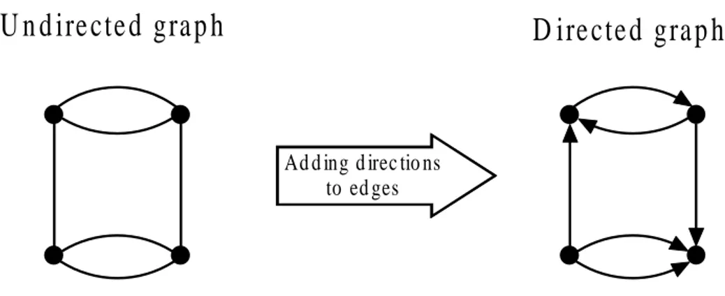
4.1.2 Positions on track
edge has a direction. Figure 15 illustrates a possible way to make the graph in Figure 14 directed. Note that the direction of an edge does not imply that movement is only possible in this direction; it is only used for representing positions on the edge.
Ad d ing d irec tio ns to ed ges
U n d ire cte d gra p h
D ire cte d gra p h
Figure 15: Example of how the undirected graph can be transformed into a directed graph.
This type of graph is called a directed multigraph and is formally defined by changing the definition of the function f to (Rosen, 1995):
f: E→{(u, v) | u, v ∈ V}
The difference is that instead of mapping each edge to a set of two nodes, it is mapped to an ordered pair of nodes. For example, if f(e) = (u, v), then u is the node at the start of edge e and v is the node at the end of edge e.
When the graph is directed, positions can be defined by an edge and an offset from the start of the track piece it represents. The infinite set of possible positions P is defined as:
P = {(e, d) | e ∈ E, d ∈ R, 0 ≤ d ≤ w(e)}
The elements of this set can uniquely define every position on the track by an ordered pair (e, d) ∈ P, where e is the edge and d is the offset from the beginning of the track piece it represents. Note that the offset d must be between 0 and w(e), which corresponds to the start position of the track piece, defined by (e, 0), and the end position of the track piece, defined by (e, w(e)), respectively. This is illustrated in Figure 16 for a track piece represented by the edge e. The arrowed line is the track piece and a is the start position and b is the end position of this track piece. The position p is defined by (e, d).
d
b
a
p
w (e )
Figure 16: Illustration of a track piece where a is the start position and b is the end position. The
position p is defined by the ordered pair (e, d), where e is the edge representing the track piece and d is the distance from the start position a to the position p on the track piece.
4.1.3 Visualization
One important goal is that the representation can be used for visualization and the current representation can be used without modifications. For example, if the track is split up as shown in Figure 17, then each track piece is formed either as an arc or as a straight line. By storing coordinates for every node and the shape of every track piece, the track layout can be visualized as it looks in the real world. This extends to all types of track-based systems as long as it can be divided into track pieces where the shape of every track piece can be represented.
Figure 17: Split points are marked with filled circles.
4.2 Dynamic
objects
In this section, dynamic objects are modeled. Dynamic objects are objects that can change their state over time, e.g. trains, switches, and sensors. From now on, the words edge and track piece are used interchangeably, e.g. movement along an edge really means movement along the track piece represented by that edge.
4.2.1 Train movement
Before going into train movement, we start by defining positive and negative movement along an edge. This is illustrated in Figure 18. If a train is going in the same direction as the direction of the edge, then it moves in the positive direction of the edge (see Figure 18a) and if it is going in the opposite direction, then it moves in
a)
b)
Figure 18: a) A train going in the positive direction of an edge. b) A train going in the negative
direction of an edge.
A problem arises when part of a train is on one edge while another part is on another edge. This is solved by moving the extremity points of a train the same distance independently of each other. This has reduced the problem of moving a train to moving two points along the track. To do this it must be decided which point is the start point and which is the end point of the train, which may be done arbitrarily. When a train is moved its start point and end point are moved the same distance. The calculation of this distance depends on how the velocity varies over time and is application dependent. First, the start point is moved and then the end point is moved as illustrated in Figure 19. When the start point is moved there is a zone between the old position and the new position called the occupied zone. In the same way, the zone between the old position and new position of the end point is called the unoccupied
zone. All sensors in the occupied zone are activated and all sensors in the unoccupied
zone are deactivated (more on this in Section 4.2.4). Collisions between trains are also checked for in this way. If another train has its start point or end point in the occupied zone, then the trains have collided. Collision detection is covered in more detail in Section 4.2.2. occu p ied zon e un o ccup ied zon e T im e t1 T im e t2 M o ve s tar t po int M o ve en d p o in t d d
Figure 19: Illustration of a train that is moved the distance d between the two consecutive time steps t1
and t2.
This approach for moving trains is easy to extend to systems that are more complicated by using more than two points for each train. For example, if it is desirable to detect when two trains are dangerously near each other, two extra points can be used for a safety interval surrounding each train. Further, some sensors may only be activated at some interval of the train (which is the case for the model
railroad, described in Section 2.3). Two extra points can be used for a sensor activation interval. An example of this is illustrated in Figure 20.
S ens or ac tivation interval T rain
S afety interval
Figure 20: Example of different intervals. Sensors are activated in the ”Sensor activation interval” and
collision detection is done in the “Safety interval”. 4.2.2 Detecting critical states
A critical state is, for example, when two trains collide or when a train derails. If the simulation is visualized, then it is not necessary to detect critical states, because a human operator can watch the simulation to see if it enters a critical state. However, if the simulator itself detects these states, long running tests can be performed without human supervision. The following situations are considered critical states:
• When two trains collide.
• When a train is on top of a switch while that switch is thrown. • When a train runs into a switch, which is in a wrong state.
The last two of these are trivial to detect. By letting a node keep track of if a train is on top of it, the second situation can be detected. The third situation is detected if the switch is in a trains occupied zone and in a wrong state. In addition to these, there may be other situations to be considered critical states (e.g. a train running to fast in a curve), but they are application dependent and must be dealt with for the given application. However, the first situation, collision detection between trains is useful for all track-based systems. Note that this is only for detecting if a collision has occurred, but not what happens if it occurs, which is application dependant. Two approaches were considered for collision detection:
1. For each time step, move all trains and then check if collisions occurred.
2. For each time step, move one train at a time and check if it collided with another train.
Both these approaches have their advantages and disadvantages. A problem with the first approach is that a collision can be undetected if the time between two consecutive time steps is sufficiently large, as illustrated in Figure 21.
T im e t1
T im e t2
detects collisions, which are incorrect. This is illustrated in Figure 22. In this example, a collision should not be detected, so the second case (Figure 22b) is incorrect. That is, depending on the order that trains are moved a collision may be detected incorrectly. Note that this can be avoided by using some algorithm that determines which train is in front and move it first.
T im e t1 T im e t2 T im e t2 c ollis ion a) b)
Figure 22: Collision detection is order dependent. a) If the train in front is moved first, no collision is
detected (correct). b) If the train behind it is moved first, a collision is detected (incorrect).
The second approach is chosen because the problem with incorrectly detected collisions is considered less severe than the problem with undetected collisions. So far, only collisions where both trains are on the same track piece have been considered. Other scenarios are also possible, which is illustrated in Figure 23.
a)
b)
c )
Figure 23: Illustration of three different collision scenarios. a) Both trains are on the same track piece.
b) A train enters a track piece that is occupied by another train. c) Two trains pass the same node, but are not on the same track piece.
The first scenario, where both trains are on the same edge, is detected by checking the occupied zone every time a train is moved as already explained. If a train has one of its extremity points in this zone, then the trains has collided. For the second and third type this will not work, because the train collides somewhere in the middle of another train. This is solved by letting each node keep track if a train is occupying it. If another train tries to occupy a node which is already occupied by a second train, then the trains collides (cf. critical sections).
4.2.3 Switches
A switch point is a position on the track where more than two track pieces meet. If a train comes to a switch point, then multiple scenarios are possible depending on the state of the switch. An example of a switch point is illustrated in Figure 24. A train is on edge e1 and soon comes to a switch point, defined by e1, w(e1). When the switch point is reached, three scenarios are possible:
1. The train will continue from the start of edge e2 (defined by (e2, 0) going in the positive direction.
2. The train will continue from the end of edge e3 (defined by (e3, w(e3)) going in the negative direction.
3. The train will derail because switch is in a “wrong” state (e.g. the switch is set so that e2 and e3 are connected).
e1
e2
e3
Figure 24: Example of a switch point connecting the edges e1, e2, and e3.
A general representation must be able to represent all these three cases for every switch on the track. Every edge e has two extremity points, one is the start position, defined by (e, 0), and the other is the end position, defined by (e, w(e)). To uniquely identify every single extremity point on a track the set F is used, where
F = { (e, 0), (e, w(e)) | e ∈ E }.
To avoid any assumptions or limitations, switches are represented in a general way by a function s that maps the extremity points of each track piece to another extremity point, i.e. s: F → F. If the train enters the edge from the start position, then it will go in the positive direction. If the train enters the edge from the end position, then it will go in the negative direction.
So, for example: s((e1, 0)) = (e2, w(e)), means that if a train go past the start of the track piece represented by edge e1, then it will enter from the end of the track piece represented by edge e2 going in the negative direction.
Going back to the example in Figure 24, the three possibilities are defined as: 1. s((e1, w(e1))) = (e2, 0) train runs in positive direction 2. s((e1, w(e1))) = (e3, w(e3)) train runs in negative direction 3. s((e1, w(e1))) is undefined
4.2.4 Sensors
A simple sensor is defined by a single position on the track. If a train covers a sensor position, then the sensor is activated, otherwise it is deactivated. This is done when a train is moved. If the sensor position is in the occupied zone, the sensor becomes activated. Conversely, if it is in the unoccupied zone, it becomes deactivated.
It is also possible to have sensors with more complicated behavior, e.g. direction sensors that are only activated when the trains go in a certain direction or sensors that covers a range of positions. A direction sensor can be defined by a single position on the track and its activation direction (positive or negative direction on the edge). A sensor that covers a range of positions can be defined by two positions (or possibly more) on the track. If one of these positions is in a train’s occupied zone, then a counter is increased and the sensor is activated (if it is not already). If one of these positions is in a train’s unoccupied zone, then the counter is decreased and if it is zero, then the sensor is deactivated.