Black-Litterman Model: Practical Asset Allocation Model Beyond Traditional Mean-Variance

(1)

BACHELOR THESIS IN MATHEMATICS /APPLIED MATHEMATICS

Black-Litterman Model:

Practical Asset Allocation Model Beyond Traditional Mean-Variance

Authors:

SHUHRAT ABDUMUMINOV

&

DAVID EMANUEL ESTEKY

KANDIDATARBETE I MATEMATIK / TILLÄMPAD MATEMATIK

DIVISION OF APPLIED MATHEMATICS

MÄLARDALEN UNIVERSITY SE-721 23 VÄSTERÅS, SWEDEN

(2)

DIVISION OF APPLIED MATHEMATICS

______________________________________________________________________ Bachelor thesis in Mathematics / Applied Mathematics

Date: 2016-06-10 Project name:

Black-Litterman Model: Practical Asset Allocation Model Beyond Traditional Mean-Variance Authors:

Shuhrat Abdumuminov David Emanuel Esteky Supervisors:

Lars Pettersson. Senior Lecturer Professor. Anatoliy Malyarenko Reviewer:

Dr. Ying Ni. Senior Lecturer Examiner:

Dr. Linus Carlsson. Senior Lecturer Comprising:

(3)

Abstract

This paper consolidates and compares the applicability and practicality of Black-Litterman model versus traditional Markowitz Mean-Variance model. Although well-known model such as Mean-Variance is academically sound and popular, it is rarely used among asset managers due to its deficiencies. To put the discussion into context we shed light on the improvement made by Fisher Black and Robert Litterman by putting the performance and practicality of both Black-Litterman and Markowitz Mean-Variance models into test. We will illustrate detailed

mathematical derivations of how the models are constructed and bring clarity and profound understanding of the intuition behind the models. We generate two different portfolios, composing data from 10-Swedish equities over the course of 10-year period and respectively select 30-days Swedish Treasury Bill as a risk-free rate. The resulting portfolios orientate our discussion towards the better comparison of the performance and applicability of these two models and we will theoretically and geometrically illustrate the differences. Finally, based on extracted results of the performance of both models we demonstrate the superiority and

practicality of Black-Litterman model, which in our particular case outperform traditional Mean-Variance model.

(4)

Acknowledgments

It has been truly an honour to have Lars Pettersson as our supervisor and senior lecturer. We are thankful to him for seeding the idea of this thesis by sharing his insights and expertise in the field of Finance. His prompt comments and beyond expectation guidance has been invaluable in crafting our thesis. Lars is an asset to the department of mathematic, his unique combination of vast experiences, both in financial industry and academia, has given us a broad perspective of how mathematics comes into play in practice.

Let us have the pleasure to express our sincere gratitude to our supervisor, Professor Anatoliy Malyarenko not only for kindly and patiently reviewing our work many times and providing us with his constructive comments, but also for allowing us to having the privilege of being his students in different classes and be able to learn from his endless knowledge and exceptional expertise in field of mathematic. This has been a great honour and inspiration which we will always carry on with us.

Also we would like to thank our senior lecturer, Dr. Ying Ni for reviewing our work and giving us valuable feedbacks.

We take this opportunity and gratefully acknowledge the kindness and support of all the staffs and lecturers at Mälardalen University for providing us with a high quality education.

Finally, we like to extend our great appreciation to our family for their unconditional love, endless support and tremendous sacrifices, without them this journey would not be possible. We are forever indebted to their kindness.

DAVID ESTEKY & SHUHRAT ABDUMUMINOV

Västerås,10th of June 2016

(5)

1 Introduction

Harry Markowitz, known as the father of Modern Portfolio Theory (MPT) published an article “Portfolio Selection” in 1952 which eventually in 1990 he received a Nobel Prize for his work on portfolio diversification, where he grounded the foundation of the modern portfolio theory. Markowitz developed a simple yet complex mathematical model, known as Mean-Variance Model (MV). This model helps investors to select and construct the most efficient portfolio by maximizing the return for the given desired risk or minimizing the risk for a given expected return. It is assumed that rational investors prefer portfolios which yields higher ratio of return to risk [4].

The essence of modern portfolio theory lies in diversification. Investors are not only aiming to find the right security to buy, but also how to spread their wealth among those assets which validates the importance of the old proverb “Do not put all your eggs in one basket”. In order to diversify and minimize the risk, Markowitz introduced the correlation between the assets. He suggests that investors should measure the correlation coefficient between the return of various securities, which as the result eliminates the unsystematic risk and reduces volatility that generates a portfolio with a higher return for the equal or less risk as oppose to individual assets [4].

Although Markowitz model is popular among scholars and appears to be practical. Ironically, it has been rarely implemented by practitioners, due to the its flaws. In particular, when Markowitz optimizer run without constrains, it often suggests taking negative position (shorting) in different assets and results in extreme weights in portfolio. This is because it overweight’s the assets with negative correlation or high expected return and underweight the assets that has positive correlation and low expected return. Another problem is input

sensitivity, where the minor changes in inputs cause drastic changes in the outcome of the portfolios weights [20]. Therefore, minor changes in input can be very sensitive and lead to massive impact on the weights of the optimal portfolio. Markowitz model also does not incorporate investors’ confidence view. However, despite the deficiencies, Markowitz model is still widely respected and recognized as the cornerstone of the modern portfolio theory. To rectify these flaws, Fischer Black & Robert Litterman developed the so called Black-Litterman model published by Goldman Sachs & Company in 1991. They major

improvement was incorporation of investors views with the implied equilibrium return which led to a more diversified portfolio. This improvement was built upon the traditional Mean-Variance and Capital Asset Pricing Model [14].

(7)

1.1 Aim and Purpose

This study is carried out with the purpose of investigating the Black-Litterman and Mean-Variance models as well as testing and comparing the performance of portfolios optimized by these two asset allocation tools. Detailed mathematical description and derivation of

contracting the model as well as deficiencies and improvements, will be also discussed. Finally, this study attempts to bring more clarity and understanding by implementing the model on real market data. Furthermore, by extracting the obtained result we give

recommendation to choose the models that has more stability and practicality, tailored to their needs.

1.2 Methodology

For our practical implementation of the Mean-Variance and the Black-Litterman model we construct portfolios composed of 10-Swedish equities and we also estimate the risk-free interest rate using 30-days Swedish Treasury Bill over 10-year period. Two main methods used in modelling the Black-Litterman are the reverse optimization and the Bayesian approach, where the reverse optimization is used to compute equilibrium excess returns for each asset and the Bayesian approach is used to incorporates investors’ views into the model.

(8)

2 Markowitz Mean-Variance Model

2.1 Portfolio’s Mathematical Properties

Prior to advancing, it is crucial to begin by representing some of the basic definitions and then continue with the mathematical derivation of the mean-variance model. Although most of the concepts introduced here tend to be rigorous and technical, the purpose here is to give an intuitive and simple explanation so the importance and beauty of the modern portfolio theory can be appreciated.

2.1.1 Portfolio’s Notations

Let us first begin by introducing the following notations used in our derivations: 𝑤: Portfolio weight of a column vector of the size 𝑛 × 1 .

𝑅: Portfolio mean return of a column vector of the size 𝑛 × 1 . 𝑉: Covariance matrix of the size 𝑛 × 𝑛 .

σ,-: Variance of the portfolio 𝑃. 𝑅/: Expected return of the portfolio 𝑃. 1: Is a column vector of ones.

r1: Expected return on risk free assets. 𝐴3_{: Denotes the transpose of a matrix 𝐴.}

2.1.2 Portfolio’s Return and Variance

As we mentioned previously, the modern portfolio theory is based on the assumption that rational investors tend to choose the portfolio that yields highest return for the least given amount of risk (variance). In order to construct the efficient frontier, first we need to

minimize the variance of the portfolio for the given expected return. Before that let us define the following. 𝑁 is the number of assets, 𝑅₅ is the expected return on the asset i and 𝑅₆ is the return on portfolio p. Now we need to define the expected return 𝑅_/ and variance 𝜎_/-_{of our} portfolio which can be stated as follows [24]:

The expected rate of return 𝑅_/ for the portfolio stated as

𝑅_/ = (𝑤₅𝑅₅) ;

5<= = 𝑤>_𝑅.

(9)

𝜎_/- _{= 𝐸 𝑟} /− 𝑅/ - = 𝐸 𝑤5(𝑟5− 𝑅5 ; 5<= ) - = 𝑤5 ; B<= ; 5<= 𝑤B𝜎5B = 𝑤>_𝑉𝑤.

Observe that 𝜎_5B is the covariance between the asset 𝑖 and 𝑗 and 𝑉 is the covariance matrix.

2.1.3 Covariance and Correlation Coefficient

Covariance is significant component of the portfolio theory, which measures how two asset moves up or down in tandem. Positive covariance means that two assets move together while the negative covariance implies that two assets move in the opposite direction. It is important to note, that when constructing a portfolio of assets, we should consider the covariance between those assets. Covariance enable us to measure the variance of the portfolio. However, when considering just one asset, then estimating the expected future return and future variance alone is sufficient. In order to have a well-diversified portfolio it is crucial to have assets with negative covariance, since when the return of one security falls, the return of the opposite security goes up and therefore it off set the potential loss [4]. However,

covariance should not be confused with correlation coefficient, which represent the degree of how much those two assets rise or fall with respect to each other and it ranges between −1 to +1 where it defines by

𝜌

_5,B

=

HIJ

H_IH_J

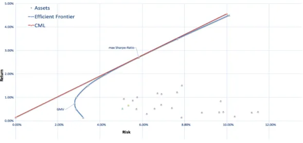
2.3 Efficient Frontier

The efficient frontier is the curve which consists of all the portfolios that generate highest return for the given level of risk in the set of all portfolios. The efficient frontier lies between the global minimum variance portfolio and the tangency portfolio. For graphical

interpretation of the different portfolio, see Figure 2.1. Therefore, portfolios that lies below the efficient frontier are not optimal since they generate less return for the subjected level of risk [24].

(10)

Figure 2.1. Efficiency frontier by Mean-Variance Model

As the result, the portfolios that are on the efficient frontier curve tend to be more diversified. The efficient frontier can be obtained by minimizing the variance of the portfolio 𝜎_/-_subject to two constrains: First, all weights must add up to one ; 𝑤₅

5<= = 1 meaning we are fully invested. Second, the portfolio has to earn expected rate of return equal to 𝑅/ [24]

Minimize 𝜎_/- _{= 𝑤}K_𝑉𝑤 Subject to 𝑤K_{𝑅 = 𝑅}

/ (2.1) 𝑤K_{1 = 1}

Now we use the method of Lagrange multipliers to solve the problem where 𝜆 denote the Lagrange multiplier [1] The Lagrangian is given by

𝐿 = 𝑤K_{𝑉𝑤 − 𝜆}

= 𝑤K𝑅 − 𝑅/ − 𝜆- 𝑤K1 − 1 (2.2) we can see that 𝑤K_{𝑉𝑤 is convex since 𝑉 is positive definite and symmetric. See (Appendix} A) for convex function. Now we need to obtain First Order Condition.

The F.O.C. are as follows 𝜕𝐿

𝜕𝑤 = 2𝑉𝑤 − 𝜆=𝑅 − 𝜆-1 = 𝟎,

(2.3)

observe that 𝟎 in (2.3) is an 𝑛 × 1 vector of zeroes 𝜕𝐿

𝜕𝜆₌ = 𝑅/− 𝑤K𝑅 = 0 ⇒ 𝑅/ = 𝑤K𝑅,

(2.4)

(11)

𝜕𝐿

𝜕𝜆₌ = 1 − 𝑤K1 = 0 ⇒ 1 = 𝑤K1,

(2.5)

we solve for 𝑤 in equation (2.3) and we obtain

𝑤 =1 2𝑉S= 𝜆=𝑅 + 𝜆-1 = 1 2𝑉S= 𝑅 1 𝜆= 𝜆- . (2.6)

Observe that we wrote the equation 𝜆₌𝑅 + 𝜆_-1 in matrix form since we use (2.4) and (2.5) to solve 𝜆_𝜆=

- , now we can write (2.4) and (2.5) as

𝑅 1 3𝑤 = 𝑅₁/ . (2.7)

Now we multiply both side of the equation (2.6) by 𝑅 1 3, then we use (2.7) to obtain

𝑅 1 3𝑤 =1

2 𝑅 1 3𝑉S= 𝑅 1 𝜆₌

𝜆_- = 𝑅1/ .

(2.8)

For convenience let us introduce notation 𝐴

𝐴 ≡ 𝑅 1 3_𝑉S= _{𝑅 1 ,} _(2.9)

which is a (2×2) symmetric matrix with components 𝑅3_𝑉S=_{𝑅 = 𝑎 , 1}3_𝑉S=_{1 = 𝑐 and} 𝑅3_𝑉S=_{1 = 𝑅}3_𝑉S=_{1 = 𝑏, and the determinant will be 𝐷 = 𝑎𝑐 − 𝑏}

-𝐴 = 𝑅Y𝑉S=𝑅 𝑅Y𝑉S=1

𝑅Y_𝑉S=_{1 1}Y_𝑉S=₁ = 𝑎 𝑏_{𝑏 𝑐} (2.10) now 𝐴 is positive definite since

𝑦₌ 𝑦_- _𝐴 𝑦=

𝑦_- = 𝑦= 𝑦- 𝑅 1 3𝑉S= 𝑅 1 𝑦_𝑦= - = 𝑦₌𝑅 + 𝑦_-1 3_𝑉S= _𝑦

=𝑅 + 𝑦-1 > 0 by the positive definiteness of 𝑉S=_{. Now we substitute 𝐴 in (2.8) to obtain}

1 2 𝐴 𝜆= 𝜆- = 𝑅 / 1 .

Since 𝐴 is non-singular and invertible, we can now solve for the multiples 1

2 𝜆₌

𝜆_- = 𝐴S= 𝑅1/

(2.11)

to achieve the desired result, we use (2.11) in (2.6). As the result, we can see that the 𝑛-vector of portfolio weights 𝑤, which minimizes portfolio variance for a given mean return is

(12)

𝑤 =1 2𝑉S= 𝑅 1 𝜆= 𝜆- = 𝑉 S= _{𝑅 1 𝐴}S= 𝑅/ 1 (2.12)

2.4 Minimum Variance Portfolio

The portfolio that has the least amount of risk invested, is called the minimum Variance Portfolio (MVP). In this case investor chooses a portfolio on the efficient frontier that has the minimum variance and it can be found by minimizing the variance subject to our budget constraint where the investor is fully invested. The minimization problem can be express as Minimize 𝜎_/- _{= 𝑤}K_𝑉𝑤

Subject to 𝑤K_{1 = 1}

to find the minimum variance portfolio with a mean return 𝑅_/ we use our definition of variance 𝜎_/-_{and matrix 𝐴 in (2.9) with the result of the portfolio weights 𝑤 which we can be} obtained from (2.12). 𝜎_/- _{= 𝑤}K_𝑉𝑤 = 𝑅/ 1 𝐴S= 𝑅 1 3𝑉S=𝑉𝑉S= 𝑅 1 𝐴S= 𝑅₁/ = 𝑅/ 1 𝐴S= 𝑅₁/ = 𝑅/ 1 _{𝑎𝑐 − 𝑏}1 _- _−𝑏𝑐 −𝑏_𝑎 𝑅₁/ (2.13) = 𝑎 − 2𝑏𝑅/+ 𝑐𝑅/ -𝑎𝑐 − 𝑏 -= 𝑎 𝐷− 2𝑏 𝐷 𝑅/− 𝑐 𝐷 𝑅/ -where in particular 𝐷 = 𝑎𝑐 − 𝑏- _{≠ 0.}

2.4.1 Global Minimum Variance Portfolio

In particular, one portfolio of our special interest is the Global Minimum Variance Portfolio (GMV) which is a portfolio with the least variance for any given mean return. The mean return of the global minimum is denoted by 𝑅] and it is given by minimizing the (2.13) with respect to 𝑅_/ which gives [24]

𝑅] =

𝑏 𝑐

(13)

and it’s variance denoted as 𝜎_]-_{which it can be obtained by substituting (2.14) into (2.13) that} yields 𝜎_]- ₌𝑎 − 2𝑏𝑅] + 𝑐𝑅] -𝑎𝑐 − 𝑏 -=𝑎 − 2𝑏 𝑏𝑐 + 𝑏 𝑐 -𝑎𝑐 − 𝑏 -= 1 𝑐. (2.15)

Weights of the global minimum variance portfolio is given by substituting (2.14) into (2.12) and we denote it by 𝑤_], 𝑤_] =𝑉−1 𝑅 1 𝐴 −1 𝑅₁𝐺 = 𝑉S= _{𝑅 1} 𝑐 −𝑏 −𝑏 𝑎 𝑏 𝑐 1 𝑎𝑐 − 𝑏 -=𝑉S=1 𝑐

notice the 𝑐 is the sum of elements in 𝑉S=_{, so we have}

= 𝑉S=1 13_𝑉S=₁.

(2.16)

Now another concept of our interest is the Orthogonal Portfolio. If two minimum variance portfolios 𝑤_/ and 𝑤_{_} are orthogonal then their covariance is equal to zero, that is

𝑤_𝑋K_𝑉𝑤

𝑃 = 0. (2.17)

For each minimum variance portfolio excluding the global minimum variance portfolio, there will exist a unique orthogonal minimum variance portfolio. Moreover, if the first portfolio has mean return 𝑅_/, then it’s orthogonal portfolio has a mean return 𝑅_{_}, which is

𝑅_=

𝑎 − 𝑏𝑅_/ 𝑏 − 𝑐𝑅_/

(2.18)

in order to obtain (2.18) let 𝑃 and 𝑋 to be arbitrary minimum variance portfolios which their weights 𝑤_/ and 𝑤_{_} is obtained by (2.12)

𝑤_{_} =𝑉−1 𝑅 1 𝐴−1 𝑅₁𝑋 (2.19)

(14)

𝑤_𝑋> 𝑉𝑤_𝑃 = 𝑅𝑋 1 𝐴S= 𝑅₁/ = 0 (2.20)

2.5 Tangency Portfolio

One portfolio of our most interest is the tangency portfolio, which is the most optimal efficient portfolio. It consist of merely risky assets and the investor is fully invested when 𝑤K_{1 = 1 with no borrowing and lending on the tangency point. In order to locate the} tangency portfolio, let us briefly represent the Sharpe ratio (𝜃) and the Capital Market Line (CML). Sharpe ratio can be defined as a return-risk ratio, which is the expected return per each unit of risk. The most risk-efficient portfolio has the highest Sharpe ratio slope obtained by (2.12) The Sharpe ratio is then given by [24]

𝜃 =𝑅/ − 𝑟b 𝜎/ .

(2.21)

The capital market line is a line drawn at the point of risk-free asset (0, 𝑟_b). Graphically the point where CML is tangent to efficient frontier is called tangency portfolio, which contains combination of only risky assets and the risk-free asset. In fact, the Sharpe ratio is the slope of the CML [4]. Equation for CML represented by

𝑅_/ = 𝑟_b+𝑅3/− 𝑟b 𝜎_3/ σ.

(2.22)

In order to find the tangency portfolio, we solve the following optimization problem where the mean return of portfolio 𝑃 is

𝑅/ = 𝑤K𝑅 + 1 + 𝑤K𝑅 𝑟b− 𝑟b = 𝑤K𝑅. And the variance of portfolio 𝑃 is

𝜎_/- _{= 𝑤}K_𝑉𝑤, now the optimization problem can be stated as

Minimize 𝜎_/- _{= 𝑤}K_𝑉𝑤 Subject to 𝑤K_{𝑅 = 𝑅}

/ (2.23) We use the method of Lagrange multipliers where the Lagrangian function can be written as

𝐿 𝑤, 𝜆 = 𝑤K_{𝑉𝑤 − 𝜆 𝑅}

/ − 𝑤K𝑅 = 0. (2.24)

(15)

𝜕𝐿 𝜕𝑤 = 2𝑉𝑤 − 𝜆𝑅 = 0 ⇒ 𝑤 = 𝜆 2𝑉S=𝑅, (2.25) 𝜕𝐿 𝜕𝜆 = −𝑤3𝑅 + 𝑅/ = 0 ⇒ 𝑅/ = 𝑤K𝑅, (2.26)

multiply both side of (2.25) by 𝑅3_{to obtain}

𝑅3_{𝑤 = 𝑅}3𝜆 2𝑉S=𝑅, (2.27) since 𝑤K_{𝑅 = 𝑅} /, equation (2.27) gives 𝜆 2= 𝑅_/ 𝑅3_𝑉S=_𝑅 (2.28)

to obtain the the weight vector of the tangency portfolio 𝑤3/ we substitute (2.28) into the equation (2.25)

𝑤_3/ = 𝑅/

𝑅3_𝑉S=_𝑅𝑉S=𝑅.

(2.29)

Notice the proportion invested in risk-free rate is 1 − ; 𝑤₅

5<= or 1 − 𝑤31 , where tangency portfolio is the minimum variance portfolio for which 13_𝑤

3/ = 1, and now by multiplying both side of the equation (2.29) by 13_{to obtain expected return of the tangency portfolio 𝑅}

3/ 𝑅_3/ =𝑅3𝑉S=𝑅

1Y_𝑉S=_𝑅.

(2.30)

For the variance of tangency portfolio, we have 𝜎_3/- _{= w}>_𝑉w = 𝑅/ 𝑅3_𝑉S=_𝑅 -𝑅3_𝑉S=_𝑉𝑉S=_𝑅 (2.31) = 𝑅/ -𝑅3_𝑉S=_𝑅. (2.32)

Now it becomes more evident that Sharpe ratio of tangency portfolio which is ratio of mean return and standard deviation of the return can be obtained by

𝑅_/ 𝜎_/ -= 𝑅/ -𝑅/ -𝑅3_𝑉S=_𝑅 = 𝑅3_𝑉S=_𝑅 (2.33)

(16)

3 The Black-Litterman Model

3.1 Introduction

As we mentioned in introduction the Mean Variance portfolio optimization has its deficiencies such as, input sensitivity, highly concentrated optimal portfolios, extreme changes in structure of the portfolio weights due to small change in expected returns and disregarding the personal views of investors [25].

In order to overcome those pitfalls, Black-Litterman enabled investors to incorporate their own views. The core contrast between traditional Mean-Variance and Black-Litterman is that Black-Litterman uses investors expected returns. Once we know the expected returns, we can use standard optimization techniques to create an optimal portfolio using CAPM [22]. The method used in the Black-Litterman model is called, reverse optimization [23] and is used to derive implied equilibrium excess returns [5]. The reverse optimization also allows us to combine our views about different assets that exists in our portfolio using Bayesian

approach [19] as well as our confidence about our views to generate the expected return vector.

Prior to dissecting into our calculation let us introduce the notations used Black-Litterman Model as follow

𝑤 – Weights vector Σ – Covariance matrix 𝛿 – Risk aversion parameter 𝑄 – Investor’s views vector

Π – Implied equilibrium excess return vector

𝑃 – Matrix that identifies the assets involved in investors’ view vector Ω – Uncertainty matrix about investors views

rf – Risk free rate

The Black-Litterman formula [5] is given by

∏ = 𝜏Σ S=_{+ 𝑃}3_ΩS=_𝑃 S=_{[ 𝜏Σ} S=_{Π + 𝑃}3_ΩS=_𝑄].

3.2 Bayesian Theorem

(17)

theorem is to integrate additional information into calculation process. In Black-Litterman model the Bayes’ theorem incorporates investors views into the model.

Let A and B be two events. If 𝑃 𝐵 > 0,

𝑃 𝐴 𝐵 =𝑃 𝐵 𝐴 𝑃 𝐴 𝑃 𝐵 where 𝑃 𝐴 𝐵 posterior distribution 𝑃 𝐵 𝐴 sampling distribution 𝑃(𝐵) the probability of B 𝑃(𝐴) prior distribution

One of the main assumptions of the Black-Litterman model is that the variance of the prior and conditional distributions around the actual mean are known, but the actual mean is not known. It was described as “Unknown Mean and Known Variance” in [19].

A portfolio return sample set for normally distributed random variable 𝑅₅ for 𝑖 = 1 … 𝑛 with unknown mean 𝜇 and known variance 𝜎-_{[19]. Let 𝜂 and 𝛿}-_{be the known mean and known} variance respectively of the conjugate prior distribution 𝜇. Using Bayesian theorem, we can figure out the posterior distribution and the Bayes estimator for 𝜇.

Call 𝑈 = 𝑅₅, since 𝑈~𝑁(𝑛𝜇, 𝑛𝜎-_{), the Maximum Likelihood Estimator (MLE) can be} expressed as 𝐿 𝑢 𝜇 = = -tuHv∗ exp = -uHv 𝑢 − 𝑛µ - , for – ∞ < 𝑢 < ∞

Since the probability density function for a normal random variable with mean 𝜂 and variance 𝛿-_is

𝑔 𝜇 = €•,

‚ ƒ‚„ v v…v

† -t

we get the joint density of 𝜇 and U for – ∞ < 𝑢 < ∞ and – ∞ < 𝜇 < ∞. 𝑓 𝑢, 𝜇 = 𝐿 𝑢 𝜇 ×𝑔 𝜇 = 1 2𝑛 𝜋𝜎-_𝛿-exp − 1 2𝑛𝜎- 𝑢 − 𝑛𝜇 -− 1 2𝛿- 𝑢 − 𝜂 - .

Let’s take a look to the exponent of the joint density function −_-uH=_v 𝑢 − 𝑛𝜇 -₋ =

(18)

− 1 2𝑛𝜎- 𝑢 − 𝑛𝜇 -− 1 2𝛿- 𝑢 − 𝜂 -= − 1 2𝑛𝜎-_𝛿-[ 𝑢 − 𝑛𝜇 -𝛿-+ 𝑢 − 𝜂 -𝑛𝜎-] = − 1 2𝑛𝜎-_𝛿- 𝑢-𝛿-− 2𝑢𝑛𝜇𝛿-+ 𝑛-𝜇-𝛿- + 𝑛𝜎-𝜇-− 2𝑛𝜎-𝜇𝜂 + 𝑛𝜎-𝜂 -= − 1 2𝑛𝜎-_𝛿- 𝑢-𝛿-− 2𝑢𝑛𝜇𝛿-+ 𝑛-𝜇-𝛿- + 𝑛𝜎-𝜇-− 2𝑛𝜎-𝜇𝜂 + 𝑛𝜎-𝜂- .

Factoring out 𝑛𝛿-_{+ 𝜎}-_{in the first term by adding and subtracting}u†vŒHv -†v_Hv •†v_ŒHv_Ž u†v_ŒHv - to our equation gives us −𝑛𝛿- + 𝜎 -2𝜎-_𝛿- 𝜇-− 2 𝛿-_{𝑢 + 𝜎}-_𝜂 𝑛𝛿-_{+ 𝜎}- 𝜇 − 1 2𝑛𝛿-_𝜎- 𝛿-𝜎-+ 𝑛𝜎-𝜂- + +𝑛𝛿-+ 𝜎 -2𝛿-_𝜎 -𝑢𝛿-_{+ 𝜎}-_𝜂 𝑛𝛿-_{+ 𝜎} -−𝑛𝛿-+ 𝜎 -2𝛿-_𝜎 -𝑢𝛿-_{+ 𝜎}-_𝜂 𝑛𝛿-_{+ 𝜎} -= −𝑛𝛿-+ 𝜎 -2𝜎-_𝛿- 𝜇-− 2 𝛿-_{𝑢 + 𝜎}-_𝜂 𝑛𝛿-_{+ 𝜎}- 𝜇 + 𝛿-_{𝑢 + 𝜎}-_𝜂 𝑛𝛿-_{+ 𝜎} -− − 1 2𝑛𝛿-_𝜎- 𝛿-𝜎-+ 𝑛𝜎-𝜂-− 𝑛 𝛿-_{𝑢 + 𝜎}-_𝜂 -𝑛𝛿-_{+ 𝜎} -= −𝑛𝛿-+ 𝜎 -2𝜎-_𝛿- 𝜇 − 𝛿-_{𝑢 + 𝜎}-_𝜂 𝑛𝛿-_{+ 𝜎} -− 1 2 𝑛-_𝛿- _{+ 𝑛𝜎}- 𝑢 − 𝑛𝜂 -.

So we can see that now we can split the exponent of the joint density function 𝑢 and 𝜇 as follows 𝑓 𝑢, 𝜇 = exp − 𝑛𝛿_2𝜎-_-+ 𝜎_𝛿_-- 𝜇 −𝛿_𝑛𝛿-𝑢 + 𝜎_-_{+ 𝜎}-_-𝜂 - ×- exp −_{2 𝑛}𝑢 − 𝑛𝜂_-_𝛿_-_{+ 𝑛𝜎}- -2𝜋𝑛𝜎-_2𝑛𝛿- . We have 𝑚 𝑢 =exp − 𝑢 − 𝑛𝜂 -2 𝑛-_𝛿-_{+ 𝑛𝜎} -2𝜋𝑛𝜎-_2𝑛𝛿- exp − 𝑛𝛿-_{+ 𝜎} -2𝜎-_𝛿- 𝜇 − 𝛿-_{𝑢 + 𝜎}-_𝜂 𝑛𝛿-_{+ 𝜎} - • S• 𝑑𝜇 = exp − 𝑢 − 𝑛𝜂 -2 𝑛-_𝛿-_{+ 𝑛𝜎} -2𝜋𝑛(𝑛𝛿- _{+ 𝜎}-₎ exp − 𝑛𝛿_2𝜎-_-+ 𝜎_𝛿_-- 𝜇 −𝛿_𝑛𝛿-𝑢 + 𝜎_-_{+ 𝜎}-_-𝜂 - 2𝜋𝜎-_𝛿 -𝑛𝛿-_{+ 𝜎} -𝑑𝜇 • S• .

(19)

The integral we obtained has normal density function and normal marginal density function for 𝑈 with mean 𝑛𝜂 and variance 𝑛-_𝛿-_{+ 𝑛𝜎}- _{. It follows that for 𝑈 = 𝑢 the posterior} density for 𝜇 is as follows

𝑔∗ _{𝜇 𝑢 =}𝑓 𝑢, 𝜇 𝑚 𝑢 = exp − 𝑛𝛿_2𝜎-_-+ 𝜎_𝛿_-- 𝜇 −𝛿_𝑛𝛿-𝑢 + 𝜎_- _{+ 𝜎}-_-𝜂 - ×- exp −_{2 𝑛}𝑢 − 𝑛𝜂_-_𝛿_-_{+ 𝑛𝜎}- -2𝜋𝑛𝜎-_2𝑛𝛿- exp −_{2 𝑛}𝑢 − 𝑛𝜂_-_𝛿_- _{+ 𝑛𝜎}- -2𝜋𝑛(𝑛𝛿-_{+ 𝜎}-₎ exp − 𝑛𝛿_2𝜎-_-+ 𝜎_𝛿_-- 𝜇 −𝛿_𝑛𝛿-𝑢 + 𝜎_-_{+ 𝜎}-_-𝜂 - 2𝜋𝜎-_𝛿 -𝑛𝛿-_{+ 𝜎} -𝑑𝜇 • S• = exp − 𝑛𝛿_2𝜎-_-+ 𝜎_𝛿_-- 𝜇 −𝛿_𝑛𝛿-𝑢 + 𝜎_-_{+ 𝜎}-_-𝜂 - 2𝜋𝜎-_𝛿 -𝑛𝛿-_{+ 𝜎} - , – ∞ < 𝜇 < ∞.

The obtained result implies that the mean of normal density 𝜂∗_{is equal to}†v•ŒHvŽ u†v_ŒHv and

variance 𝛿∗-_{is equal to} Hv†v

u†v_ŒHv . From this point we find that Bayes estimator 𝜇’ is

𝜇_’= 𝛿-𝑈 + 𝜎-𝜂 𝑛𝛿-_{+ 𝜎}- = 𝑛𝛿 -𝑛𝛿-_{+ 𝜎}-𝑅 + 𝜎 -𝑛𝛿- _{+ 𝜎}-𝜂.

We see that obtained Bayes estimator is a weighted average of the 𝑅, the mean of the prior 𝜂 and Maximum Likelihood Estimator 𝐿. By increasing sample size the weight of sample mean 𝑅 increases and the weight of prior mean 𝜂 decreases [19]. Applying the obtained results to the Black-Litterman Model we clearly see that the model generates posterior implied equilibrium expected returns by integration of the investors views into the prior expected returns using Bayesian method [5].

3.3 Parameter 𝜏, uncertainty of investor’s views

Let U be the standard utility function of Mean-Variance optimization function 𝑈 = 𝑤3_{Π − 0.5𝐴𝑤}3_Σ𝑤

(20)

in order to maximize the investor’s utility, we need to maximize U by taking partial derivative with respect to 𝑤 and set it equal to zero

–—

–˜= Π − =

-2𝛿Σ𝑤 = Π − 𝛿Σ𝑤 = 0. (3.2) The idea behind the Black-Litterman Model was to solve for Π (3.2) rather than solving for optimal weights 𝑤, which are already observed in the market and can be computed using market capitalization.

Thus

Π = 𝛿Σ𝑤 (3.3)

the risk aversion coefficient can also be written as

𝛿 =™ š›Sšœ

H›v (3.4)

if an investor satisfied by the excess returns generated by (3.4), the investors should hold the market portfolio if they have no particular view and the returns will bring us back to the equilibrium market weights.

An investor can have absolute view about a stock. For instance, the return of the stock 𝐴 is 𝑛 percent. The investor can also have relative views of the returns. For instance, the return of the stock 𝐵 will be grater than the return of the stock 𝐶 by 𝑘 percent.

Let assume that investor believe that asset A is going to exceed the return on asset 𝐵 by 𝑥 percent

𝑟 > 𝑟’ by 𝑥= % and let’s assume that the investor has another view that

𝑟_¡ > 𝑟 by 𝑥_- %

from this point the investors can express their views as a views vector 𝑄 with dimension 𝑛 by 1, where 𝑛 is the number of views

𝑄 = 𝑥_𝑥=

- , 𝑛 = 2, 𝑗 = 1.

The vector 𝑄 itself does not give any information of the impact of investors’ views on their portfolio performance. The views need to be integrated. Matrix 𝑃 is a matrix with 𝑛 numbers of views and 𝑗 number of observed assets. For each positive view we will fill the respective

(21)

So if we believe that return on asset 𝐴 will exceed the return on asset 𝐵, it implies that we are positive about the returns on asset 𝐴. On the other hand, the view about asset 𝐵 will be negative. Since we do not have any view about asset 𝐶 in this case, we mark respective cell by 0. Likewise, we fill the next row (Table 3.1). If the views are relative, the row of the 𝑃 matrix should sum to 0 and to 1 if the view is absolute

𝑃 = 1 −1 0

−1 0 1 , 𝑤ℎ𝑒𝑟𝑒 𝑛 = 2, 𝑗 = 3

Table 3.1. Matrix 𝑃

3.4 Views Vector and Uncertainty Matrix

Lets now focus on risk. Whenever we deal with expected returns, it is intuitively implying that we will have some level of uncertainty, which we can represent through the Variance-Covariance matrix 𝛴. On the other hand, the confidence of our expectations will be represented as ΣS=_.

We can apply the same logic for our views vector 𝑄. As we are not certain about our views, we need to add an error component to our view vector 𝑄 as follow

𝑄 + 𝜀 = 𝑥₌ . . . 𝑥_u + 𝜀₌ . . . 𝜀u

the error terms are normally distributed 𝜀~𝑁 0₀ , 𝜔_𝜔== 𝜔=B

u= 𝜔uB , where

𝜔₌₌ 𝜔_=B

𝜔_u= 𝜔_uB → Ω. The Ω represents the uncertainty about our views on excess returns. Now we deal with the problem that there is not a best way of computing Ω, however Black and Litterman [5] suggests that Ω = 𝑃(τΣ)𝑃3 where 𝜏 is a scalar. A B C VIEW 1 1 -1 0 VIEW 2 -1 0 1

(22)

3.5 The impact of 𝜏

The most mysterious part of the Black-Litterman Model is the parameter 𝜏. There are two main ways in using the parameter 𝜏 in the Black-Litterman Model. The way of specifying precise meaning in the model implies the investors’ preference of Canonical Reference Model. On the other hand, the way of choosing a random value for τ is likely using the Alternative Reference Model [20].

In their paper, He and Litterman use 𝜏 = 0.025, see [14], however other researchers use 𝜏 = 1, see [21]. In this paper we will use 𝜏 = 1, which imply that we will not figure out the uncertainty of the factor 𝜏. However, if 𝜏 is not equal to 1 then the parameter should be calibrated by Maximum Likelihood Estimator method [20], where T is the number of samples and N is the number of assets

𝜏 =₃= is a biased MLE estimator 𝜏 =_3S;= is an unbiased MLE estimator

To specify the impact of τ given canonical model lets substitute uncertainty matrix Ω into the formula of the mean returns ∏

∏ = ∏ + τΣ PY _PτΣPY _{+ Ω} S=_{[Q − PΠ}Y_] = ∏ + τΣ PY _PτΣPY _{+ PτΣP}Y S=_{[Q − PΠ}Y_] = ∏ +1 2τΣ PY PY S= PτΣ S= [Q − PΠY] = ∏ +1 2τΣ PY PY S= τΣ]S=[P S= [Q − PΠY_] = ∏ +1 2 P S= [Q − PΠY]

elimination of the 𝜏 parameter from the equation confirms the proportionality to the uncertainty matrix Ω [20].

Substituting Ω into the alternative formula posterior variance M we get M = τΣ − τΣPY _PτΣPY_{+ Ω} S=_PτΣ = τΣ − τΣ PY _PτΣPY _{+ PτΣP}Y S=_PτΣ = τΣ −1 2τΣ PY PY S= τΣ]S=[P S= PτΣ = τΣ −1 2τΣ 1

(23)

we see that the parameter 𝜏 is not eliminated from the formula. Thus 𝜏 alters the prior covariance of the returns. In the alternative model no posterior variance is calculated and the weights vector is based on the variance of returns.

Given these points, multiplying by 𝜏 adjusts the prior covariance matrix with the uncertainty of the views and do not have a negative impact on the precision of the results [20].

If Ω represents the uncertainty of our views and we want to have a measure of the confidence for our views, we simply denote the confidence measure as ΩS=_.

3.6 The Black-Litterman Formula

The main idea behind the Black-Litterman formula is that we get an estimate of excess returns by calculating a weighted average of Π and 𝑄. To be able to estimate the weighted average we need to figure out the weights first.

Recall the Black-Litterman formula

∏ = 𝜏Σ S=_{+ 𝑃}3_ΩS=_𝑃 S=_{[ 𝜏Σ} S=_{Π + 𝑃}3_ΩS=_𝑄]. _(3.5) The first weight is the confidence of Π and is represented as 𝜏Σ S=_{[10]. The second weight} is related to the confidence of our views 𝑄 as 𝑃3_ΩS=_.

So the weighted average is 𝜏Σ S=_{Π + 𝑃}3_ΩS=_{𝑄. We can see that the weighted average is the} second term of the Black-Litterman formula.

3.7 Posterior distribution of assets return

We can apply Bayesian approach to blend the prior and conditional distributions to generate a new posterior distribution of the asset returns. The posterior distribution of the

Black-Litterman model asset returns is as follows

𝑃 𝐴 𝐵 ~𝑁( 𝜏Σ S=_{Π + 𝑃}3_ΩS=_{𝑄 𝜏Σ} S=_{+ 𝑃}3_ΩS=_𝑃 S=_{, 𝜏Σ} S=_{+ 𝑃}3_ΩS=_𝑃 S=_). The Alternative Black-Litterman formula represented as

(24)

M = 𝜏Σ S=_{+ 𝑃}3_ΩS=_𝑃 S=

with the mean returns ∏ and the posterior variance M of the posterior mean estimate [20]. For the posterior covariance of the returns we need to add the variance of the distribution around the estimate and the variance of the estimate itself [20], [7]

Σ6 = Σ + 𝑀

some other researchers used known variance of the returns instead of calculating the new posterior variance [20], [10].

(25)

4 Data Implementations and Empirical Findings

In this chapter we will implement empirical data to the Black-Litterman Model and compare the outcome with obtained result from the Mean Variance Model.

4.1 Black-Litterman Model – a simple example

For illustration purpose, let us apply Black-Litterman Model on a simple case with one asset, asset A. The parameters given for the asset A as follows

Implied equilibrium excess return Π = −2%

Variance Σ = 1.1%

Predicted excess return 𝑄 = 1% Uncertainty about the view Ω = 0.25%

We use 𝜏 = 1, as long as we looking for the one asset case, the value of 𝑃-matrix will be equal to 1. ∏ = 𝜏Σ S=_{+ 𝑃}3_ΩS=_𝑃 S=_{[ 𝜏Σ} S=_{Π + 𝑃}3_ΩS=_𝑄] = 1 ∗ 0.011 S=_{+ 1}3_{∗ 0.0025}S=_{∗ 1} S=_{[ 1 ∗ 0.011} S=_{(−0.02) + 1}3_{∗ 0.0025}S= ∗ 0.01] = 0.0020371[ 90.909 −0.02 + 400 0.01 ] ≈ 0.44%.

The result is the estimate of the excepted returns using Black-Litterman formula. It becomes evident that the obtained result of 0.44% is closer to our predicted return of 1% than to the implied equilibrium excess return of -2%. Having uncertainty about our view on the level of 0.25%, which is lower than the variance of the implied equilibrium excess return of 1.1%, makes us more certain about our views, relative to the market. However, if we use a higher value for Ω, the result will be directed back towards the implied equilibrium excess return. For instance, if Ω = 100% then

∏ = 1 ∗ 0.011 S=_{+ 1}3_{∗ 0.01}S=_{∗ 1} S=_{[ 1 ∗ 0.011} S=_{(−0.02) + 1}3_{∗ 0.01}S=_{∗ 0.01]} ≈ −2%.

Using Black-Litterman method we get the possibility to reflect our views on the expected excess returns to optimize the portfolio.

(26)

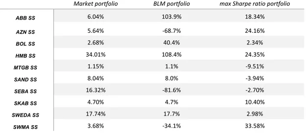
4.2 Black-Litterman Model – implementation to Swedish market

We have chosen 10-Swedish equities, and 30-days Swedish Treasury Bill as a risk-free rate. The historical data for period October 2004 to October 2014 obtained from the Nasdaq OMX Nordic. The risk aversion coefficient 𝛿 has been calculated using (3.4) and is set to be

constant at the level of 2.81. Covariance matrix of the observed assets is calculated as shown in (Table 4.1). ABB SS AZN SS BOL SS HMB SS MTGB SS SAND SS SEBA SS SKAB SS SWEDA SS SWMA SS ABB SS 0.47% 0.02% 0.47% 0.08% 0.38% 0.29% 0.28% 0.21% 0.26% 0.08% AZN SS 0.02% 0.32% -0.03% 0.01% -0.01% -0.01% 0.01% 0.00% 0.04% -0.01% BOL SS 0.47% -0.03% 2.38% 0.18% 0.67% 0.70% 0.76% 0.39% 0.62% 0.15% HMB SS 0.08% 0.01% 0.18% 0.31% 0.23% 0.13% 0.14% 0.15% 0.17% 0.05% MTGB SS 0.38% -0.01% 0.67% 0.23% 1.24% 0.47% 0.51% 0.46% 0.78% 0.11% SAND SS 0.29% -0.01% 0.70% 0.13% 0.47% 0.77% 0.45% 0.34% 0.47% 0.07% SEBA SS 0.28% 0.01% 0.76% 0.14% 0.51% 0.45% 0.92% 0.35% 0.86% 0.05% SKAB SS 0.21% 0.00% 0.39% 0.15% 0.46% 0.34% 0.35% 0.54% 0.39% 0.01% SWEDA SS 0.26% 0.04% 0.62% 0.17% 0.78% 0.47% 0.86% 0.39% 1.30% 0.08% SWMA SS 0.08% -0.01% 0.15% 0.05% 0.11% 0.07% 0.05% 0.01% 0.08% 0.26%

Table 4.1. Variance Covariance Matrix

The next step is to figure out the market weights of the assets using the historical market capitalization data, the vector of the implied volatility excess returns Π and betas of the particular assets, the data shown in (Table 4.2). It is important to mention that for simplicity we assume that the market consists of only 10-Swedish equities (risky assets) and the 30-days Swedish Treasury Bill (risk-free asset).

VARIANCE 𝛃 COVAR(RI,RM) MKT.CAP BLN.USD MKT.WEIGHTS 𝚷 HISTORICAL AV.RETURNS

ABB SS 0.48% 0.83 0.21% 74.16 6.04% 0.57% 1.40% AZN SS 0.33% 0.11 0.03% 69.26 5.64% 0.08% 0.67% BOL SS 2.40% 1.76 0.45% 32.88 2.68% 1.33% 2.34% HMB SS 0.31% 0.62 0.16% 417.62 34.01% 0.54% 1.03% MTGB SS 1.25% 1.47 0.38% 14.06 1.15% 1.18% 0.97% SAND SS 0.78% 1.32 0.34% 98.7 8.04% 0.91% 0.75% SEBA SS 0.93% 1.37 0.35% 200.43 16.32% 1.26% 0.86% SKAB SS 0.55% 0.97 0.25% 57.7 4.70% 0.73% 0.82% SWEDA SS 1.32% 1.53 0.39% 217.87 17.74% 1.50% 1.00% SWMA SS 0.26% 0.24 0.06% 45.14 3.68% 0.18% 1.07%

(27)

The vector of implied equilibrium excess returns Π obtained by reverse optimization method. We used the historical market capitalization data to obtain the market weights thereafter we find Π using (3.3).

If we do not have our own views on the assets performance we can use Π and the standard Mean-Variance optimization technique to create an optimum portfolio. Return vector Π will refer back to the market weights and we basically will obtain a market portfolio.

4.2.1 The impact of the view on expected return

If we have our own views (Table 4.3), for instance, we believe that ABB will outperform SEBA by 3%, BOL outperform SWMA by 5% and HMB outperform AZN by 3% then the impact on the return vector will be as shown in Figure 4.1.

Q _{ABB SS} _{AZN SS} _{BOL SS} _{HMB SS} _{MTGB SS} _{SAND SS} _{SEBA SS} _{SKAB SS} _{SWEDA SS} _{SWMA SS}

3.00% View 1 1 0 0 0 0 0 -1 0 0 0

5.00% View 2 0 0 1 0 0 0 0 0 0 -1

3.00% View 3 0 -1 0 1 0 0 0 0 0 0

Table 4.3. Investor’s view and P-matrix

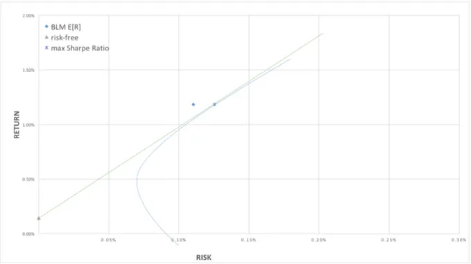
Figure 4.1. Return vectors

From Figure 4.1 we can see the reflection of the investor’s view on the expected return vector. First of all, we see how far CAPM expected returns from the historical average returns. Secondly, we can see from this figure how our views are reflected on the return

(28)

vectors. We assume that ABB outperform SEBA – the BLM increases the value of the expected return for ABB and decreases for SEBA. The same result we see in case of BOL and SWMA, HMB and AZN.

4.2.2 Diversification possibility by Black-Litterman Model

Using historical average returns of the assets and Mean-Variance Model we find the weights vector of the tangency portfolio, which is by definition is the most efficient portfolio by Mean-Variance portfolio optimization model. The portfolio lies on the CML line and by definition no other portfolios lies to the left of the CML line. In this paper we will show that for given data set using Black-Litterman Model(BLM) it is possible to create a portfolio with the same amount of return for the lower risk.

In (Table 4.4) we have shown the weight vectors for observed portfolios

Market portfolio BLM portfolio max Sharpe ratio portfolio

ABB SS 6.04% 103.9% 18.34% AZN SS 5.64% -68.7% 24.16% BOL SS 2.68% 40.4% 2.34% HMB SS 34.01% 108.4% 24.35% MTGB SS 1.15% 1.1% -9.51% SAND SS 8.04% 8.0% -3.94% SEBA SS 16.32% -81.6% -2.70% SKAB SS 4.70% 4.7% 10.40% SWEDA SS 17.74% 17.7% 2.98% SWMA SS 3.68% -34.1% 33.58%

Table 4.4. Weight vectors

Using maximum Sharpe ratio portfolio as the benchmark to compare with the BL portfolio, we can see that for the same level of return the BL portfolio has lower risk – the portfolio is more diversified (Figure 4.2).

(29)

Figure 4.2. Portfolio by Black-Litterman Model

By analysing the weight vectors that we previously obtained we can observe that the amount of each asset varies when we have different views, for instance increase in those assets with positive views and decrease in assets with negative views, see (Table 4.4). It allows the investor to reach the higher level of utility by implementing an additional information to the estimation process, see (Figure 4.2). However, this is not an investment recommendation and the rate of return may differ from our result if the investors have different views about observed stocks performance. Our result shows the importance of use of the external real-time data analysis in order to implement it to the portfolio performance estimation process and possibility to outperform the classical Mean-Variance Model.

(30)

5 Conclusion and Recommendation

We have investigated the impact of the future expectations of assets performance on the portfolio created using Mean Variance model, which basis the optimization method on the empirical data. By creating different portfolios, we have shown that using Bayesian approach, the Black-Litterman model incorporates the investors’ personal views into portfolio

optimization process.

By analysing the weight vectors that we previously obtained we can observe that the amount of assets varies when we have different views, for instance increase in those assets with positive view and decrease in assets with negative view. That implies Black-Litterman model generates more diversified portfolio by maintain same level of return as oppose to traditional Mean-Variance model. Another interesting conclusion derived from our research is that the portfolio optimization which is based on the Mean-Variance model is relatively bounded by CML as opposed by the Black-Litterman model which can outperform the MV portfolio. As we have seen the BL portfolio can give higher return by the same amount of risk.

Based on our observations we recommend assent managers to not only rely on the historical data, which is also sometimes it is difficult to obtain, but also use the up-to-date analysis to diversify the portfolio using the Black-Litterman model. In the rapidly changing world the adjustment for the expected change plays significant role in portfolio optimization.

6 Further Research

For further research it would be interesting while creating portfolio to take into account the behaviour of the investor based on the level of his or her professional skills and experience. As we have shown the up-to-date analysis has a crucial impact on the performance of the portfolio, but the level of confidence of the investors is not distinguished from each other during the estimation process.

(31)

7 Fulfilment of Thesis Objectives

In this section authors provides a brief deceleration of the fulfilment of 6 objectives achieved in this thesis, required by the Swedish National Agency for Higher Education.

Objective 1

For Bachelor degree, students should demonstrate knowledge and understanding in the major field of study, including knowledge in the fields’ scientific basis, knowledge of applicable methods in the field of specialization in some part of the field and orientation in current research questions.

Fulfilment: The authors demonstrated their knowledge and understanding in the area of

mathematics by applying and presenting detailed mathematical methods, proofs and examples in i.e. proof of the Lagrange multipliers theory, Bayesian method of estimating posterior probability measure, solve the portfolio optimization problems and dissect the intuition and practical use behind Black-Litterman and Mean-Variance asset allocation model. With a step by step explanation of mathematical derivation behind portfolio theory, real-market data has been incorporated using those derivations in Microsoft Excel software in order to compare the results of the models.

Furthermore, the authors discuss the advantages and disadvantages Black-Litterman and Mean-Variance model.

Objective 2

For Bachelor degree, the student should demonstrate the ability to search, collect, evaluate and critically interpret information in a problem formulation and to critically discuss phenomena, problem formulations and situations.

Fulfilment: The authors has been rigorously researched the related topic using different academic search engines as well as lecture notes and related books. The collected useful and interesting scientific papers and journals later has been critically reviewed, interpret and referred to. The authors have also collected relevant market data and implemented the model using the data. By gathering different pieces of information from different sources authors have been able to evaluated the information and formulate the problem in a clear and structured fashion.

Objective 3

For Bachelor degree, the student should demonstrate the ability to independently identify, formulate and solve problems and to perform tasks within specified time frames.

Fulfilment: The authors have met the dead lines throughout the process of writing the thesis

(32)

Objective 4

For Bachelor degree, the student should demonstrate the ability to present orally and in writing and discuss information, problems and solutions in dialogue with different groups.

Fulfilment: This objective will be meet on the day of presentation on June 10th 2016 at Mälardalen University in Västerås.

Objective 5

For bachelor degree, the student should demonstrate ability in the major field of study make judgments with respect to scientific, societal and ethical aspects.

Fulfilment: To the best of our knowledge we have performed and demonstrate our ability to

(33)

Bibliography

[1] A. R. Alexander ,C. Essex. Calculus: a complete course. Addison- Wesley, 1999.   [2] M. Charlotta. The Black–Litterman Model: mathematical and behavioural finance approaches towards its use in practice. PhD thesis, KTH.  

[3] J. Danielsson. Financial Risk Forecasting. Wiley, 2011.  

[4] E. J. Elton, M. J. Gruber, S. J. Brown, and W. N. Goetzmann. Modern portfolio theory and Investment Analysis. International Student Version. 8th Edition. John Wiley and Sons Inc, 2011. 

[5] F. Black, R. Litterman. Global portfolio optimization. Financial Analysts Journal 48, Vol. 5, 1992.  

[6] R. Grinold, R. Kahn. Active Portfolio Management: A Quantitative Approach for

Producing Superior Returns and Selecting Superior Returns and Controlling Risk. McGraw Hill, 1999.  

[7] G. He, R. Litterman. “The Intuition Behind Black-Litterman Model Portfolios.” Investment Management Research, Goldman, Sachs & Company, 1999.

[8] H.V. Henderson, S.R. Searle. On deriving the inverse of a sum of matrices. Siam, 1981.   [9] A. Howard, C. Rorres. Elementary linear algebra. John Wiley & Sons, 2011.  

[10] T. M. Idzorek. A step-by-step guide to the Black–Litterman model. Zephyr Associates, Inc., 2002.  

[11] L. Moshe, R. Richard. The market portfolio may be mean/variance efficient after all. Review of Financial Studies, 2010.  

[12] A.W. Lo. The statistics of Sharpe ratios. Financial Analysts Journal, 2002.   [13] H. Markowitz. Portfolio selection. The Journal of Finance, Vol.7, 1952.

[14] G. He, R. Litterman. The Intuition Behind Black Litterman Model Portfolios, Goldman, Sachs & Co., 2002.

[15] W.F. Sharpe. The Sharpe ratio. The journal of portfolio management, Vol. 7, 1994. [16] S. Satchell, A. Scowcroft. A demystification of the Black–Litterman model: Managing quantitative and traditional portfolio construction. Journal of Asset Management, Vol. 17, 2000.  

(34)

[17] J. Stewart. Calculus Early Transcendentals. Cengage Learning, 2012.  

[18] W. F. Trench. Introduction to Real Analysis. Prentice Hall/Pearson Education, 2003.   [19] D. Wackerly, W. Mendenhall and Richard L.Scheaffer. Mathematical Statistics with Applications. Cengage Learning, 2007.  

[20] J. Walters. The Black–Litterman Model in Detail, Jay Walters, CFA, 2014.

[21] S. Satchell, A. Scowcroft. A Demystification of the Black-Litterman Model: Managing Quantitative and Traditional Portfolio Construction. Journal of Asset Management, Vol 1, 2, 2000.

[22] W. F. Sharpe. Capital Asset Prices: A Theory of Market Equilibrium. Journal of Finance, September, 1964.

[23] W. F. Sharpe. Imputing Expected Security Returns from Portfolio Composition. Journal of Financial and Quantitative Analysis, June, 1974.

[24] G.M. Constantinides, A.G. Malliaris, Handbooks in Operations Research and Management Science, Vol 9, Elsevier. 1995.

[25] S. Satchell. Forecasting expected returns in the financial markets. Oxford: Elsevier/AP., 2007

(35)

List of Figures

Figure 2.1 Efficiency frontier by Mean-Variance Model ………6 Figure 4.1 Weights vector ………….……….23 Figure 4.2 Portfolio by Black-Litterman Model……….25

(36)

List of Tables

Table 3.1 Matrix 𝑃……….…. 17

Table 4.1 Variance-Covariance matrix ………...22

Table 4.2 Historical data……….….23

Table 4.3 Investor’s view and 𝑃-matrix………...23

(37)

Appendix A.

Let 𝐷 be a subset of the space ℝu_{. 𝐷 is called convex if for all 𝒙, 𝒚 ∈ 𝐷 and for all 𝜆 ∈ 0,1} we have 𝜆𝒙 + 1 − 𝜆 𝒚 ∈ 𝐷.

Let 𝑓: 𝐷 → ℝ. 𝑓 is called strictly convex if for all 𝒙, 𝒚 ∈ 𝐷 with 𝒙 ≠ 𝒚 and for all 𝜆 ∈ (0,1) we have

𝑓(𝜆𝒙 + 1 − 𝜆 𝒚) < 𝜆𝑓 𝒙 + 1 − 𝜆 𝑓 𝒚 .

Let 𝐴 be a positive-definite matrix, and let 𝑓 𝒙 = 𝒙3_{𝐴𝒙. Then 𝑓 is strictly convex.} Indeed, let 𝒙, 𝒚 ∈ 𝐷 with 𝒙 ≠ 𝒚, where 𝐷 is convex. It is enough to prove that

𝐹 ≔ 𝜆𝑓 𝒙 + 1 − 𝜆 𝑓 𝒚 − 𝑓(𝜆𝒙 + 1 − 𝜆 𝒚) > 0. We have 𝐹 = 𝜆𝒙3_{𝐴𝒙 + 1 − 𝜆 𝒚}3_{𝐴𝒚 − 𝜆𝒙}3_{+ 1 − 𝜆 𝒚}3 _{𝐴 𝜆𝒙 + 1 − 𝜆 𝒚} = 𝜆𝒙3_{𝐴𝒙 + 1 − 𝜆 𝒚}3_{𝐴𝒚 − 𝜆}-_𝒙3_{𝐴𝒙 − 𝜆(1 − 𝜆)𝒙}3_𝐴𝒚 − 1 − 𝜆 𝜆𝒚3_{𝐴𝒙 − 1 − 𝜆} -_𝒚3_𝐴𝒚 = 𝜆𝒙3_{𝐴𝒙 − 𝜆}-_𝒙3_{𝐴𝒙 + [ 1 − 𝜆 𝒚}3_{𝐴𝒚 − 1 − 𝜆} -_𝒚3_𝐴𝒚] −𝜆(1 − 𝜆)[ 𝒙3_{𝐴𝒚 + 𝒚}3_𝐴𝒙] = 𝜆 1 − 𝜆 [𝒙3_{𝐴𝒙 + 𝒚}3_{𝐴𝒚 − 𝒙}3_{𝐴𝒚 − 𝒚}3_𝐴𝒙] = 𝜆 1 − 𝜆 𝒙3_{− 𝒚}3 _{𝐴(𝒙 − 𝒚) > 0,}

Because 𝜆 > 0, 1 − 𝜆 > 0, 𝒙 − 𝒚 ≠ 𝟎 and 𝐴 is positive definite.

If a function 𝑓 is strictly convex on 𝐷, then it cannot have more than one minimum.

Indeed, assume it has two minima at points 𝒙 and 𝒚. Then, by definition of strictly convex function, for any 𝜆 ∈ 0,1 we have

𝑓 𝜆𝒙 + 1 − 𝜆 𝒚 < 𝜆𝑓 𝒙 + 1 − 𝜆 𝑓(𝒚) = 𝜆𝑓 𝒙 + 1 − 𝜆 𝑓 𝒙 = 𝑓 𝒙 ,

that is, the value of 𝑓 at the point 𝜆𝒙 + 1 − 𝜆 𝒚 is less that its minimal value. The source of contradiction is our assumption about existence of more than one minimum.