Performance Measurements in Wireless 802: 11g Multi-Hop Networks

(1)

MASTER’S THESIS

Performance Measurements in Wireless

802.11g Multi-Hop Networks

prepared for the

H¨

ogskolan i Halmstad

Degree Program

International Master’s Programme in Computer Systems Engineering

or Electrical Engineering

submitted by:

Stefan Achleitner and Wolfgang Seiss

Head of Faculty:

J¨orgen Carlsson

Supervisor:

Urban Bilstrup

(2)

(3)

Details

First Name, Surname: Stefan Achleitner and Wolfgang Seiss

University: H¨ogskolan i Halmstad

Degree Program: International Master’s Programme in

Com-puter Systems Engineering or Electrical En-gineering

Title of Thesis: Performance Measurements in Wireless

802.11g Multi-Hop Networks

Academic Supervisor: Urban Bilstrup

Keywords

1. Keyword: Wireless Multi-Hop Network

2. Keyword: Performance Measurements

3. Keyword: Changing Environment

Abstract

This paper deals with performance measurements in 802.11g Wireless Multi-Hop Net-works at different locations. After an introduction to 802.11g Wireless LANs and Wireless Multi-Hop Networks, the testing environment consisting of hardware, soft-ware, configuration, and three different locations is described. Before test series for the actual measurements are defined, carried out reference tests provide reference perfor-mance data and prove that the used hardware is suitable for testing Wireless Multi-Hop Networks. Then the results of the measurements are discussed which show the influ-ence of multiple hops on throughput and latency for single and multi channel Multi-Hop Networks in indoor, outdoor, and urban environment. Finally, an outlook to further tests and improvements of Wireless Multi-Hop Networks is given.

(4)

(5)

Acknowledgement

In theory, there is no difference between theory and practice. But, in practice, there is.

Jan L. A. van de Snepscheut (1953 – 1994)

Writing this thesis gave us a deeper understanding of the behaviour of wireless networks in ideal and real life environment and an insight into Wireless Multi-Hop Networks. Especially working with real hardware and carrying out real tests instead of only sim-ulating Multi-Hop Networks was a great opportunity for us.

We therefore want to thank our supervisor Urban Bilstrup for supporting us during all the time of the thesis work. He not only provided knowledge, but also helped us with the outdoor measurements at the beach of Tyl¨osand, where we spent quite some hours. Finally, we thank our parents for making it possible to study in another country and our friends at home for their patience in this time of staying abroad.

Stefan Achleitner Wolfgang Seiss

Halmstad, 29th _{May 2006}

(6)

(7)

4 Testing Environment 17 4.1 Hardware . . . 17 4.1.1 Routers . . . 17 4.1.2 Wireless Parameters . . . 18 4.1.3 Computers . . . 18 4.2 Locations . . . 19 4.3 Software . . . 20 4.3.1 Ping . . . 22 4.3.2 Iperf . . . 23 4.3.3 NetPIPE . . . 23 5 Measurements 25 5.1 Test Sequence . . . 25 5.2 Reference Tests . . . 26 5.2.1 Hardware Tests . . . 26 5.2.2 Multi-Hop Tests . . . 27 5.2.3 Wireless Tests . . . 32 5.2.4 Conclusion . . . 32 5.3 Test Series . . . 34

5.3.1 Wireless Multi-Hop Tests using One Channel . . . 34

5.3.2 Wireless Multi-Hop Tests using Several Channels . . . 36

5.3.3 Wireless Multi-Hop Tests in Urban Environment . . . 38

(9)

6 Discussion of the Results 39

6.1 Throughput on a Single Wireless Link . . . 39

6.2 The Influence of Multiple Hops on Throughput and Latency . . . 41

6.2.1 Comparison of Maximum UDP and TCP Throughput . . . 41

6.2.2 Maximum Throughput and Latency . . . 42

6.2.3 The Behaviour of a TCP Stream in a Wireless Multi-Hop Network 45 6.3 Indoor vs. Outdoor Environment . . . 47

6.3.1 Impact of the Environment on the Throughput . . . 47

6.3.2 Impact of the Environment on the Round Trip Time . . . 47

6.4 Advantages and Disadvantages of Utilizing Several Channels . . . 50

6.5 Urban Environment . . . 52

6.5.1 Maximum TCP Throughput . . . 52

6.5.2 Behaviour of a TCP Stream in Urban Environment . . . 54

6.5.3 Round Trip Time in Urban Environment . . . 56

7 Outlook 59 7.1 Further Measurements . . . 59

7.2 Modifications of the MAC-Layer . . . 60

8 Summary 61

Bibliography 63

List of Abbreviations 69

(10)

(11)

List of Figures

2.1 Ad hoc Mode . . . 4

2.2 Infrastructure Mode . . . 5

2.3 802.11 Medium Access . . . 6

3.1 Transmission and Interference Range of a Single Channel WMHN . . . 10

3.2 Simultaneous Transmissions on a Multi Channel WMHN . . . 11

3.3 Wireless Mesh Network . . . 12

3.4 Route Reply and Route Request in AODV . . . 14

3.5 MultiPoint Relaying in OLSR . . . 15

4.1 Testing Location at the Beach of Tyl¨osand . . . 20

4.2 Map of the Wireless Test Setup in an Urban Environment . . . 21

4.3 Sequence Diagram of PING . . . 22

5.1 Maximum TCP Throughput vs. Median RTT of the Hardware . . . 27

5.2 Network Topology of the LAN Reference Tests . . . 28

5.3 Throughput, Signature, and Saturation Graph of a Wired MHN . . . . 29

5.4 TCP Throughput and Median RTT depending on the Number of Routers 31 5.5 Maximum TCP Throughput of Two Routers on LAN and WLAN . . . 33

5.6 Two IP-Networks on a Single Shared Interface . . . 34

5.7 Network Topology for the Multi-Hop Tests using One Channel . . . 35

5.8 Network Topology for the Multi-Hop Tests using Several Channels . . . 37

6.1 Behaviour of a TCP stream at different Link-Layer Speeds . . . 40

6.2 UDP vs. TCP Throughput Depending on the Number of Links (54 MBit/s) 42 6.3 Impact of Multiple Hops on TCP Throughput and Median RTT . . . . 44 6.4 Behaviour of a TCP Stream for a Varying Number of Links at 54 MBit/s 46

6.5 Throughput Graph of the Indoor and Outdoor Environment at 54 MBit/s 48

(12)

6.6 Median RTTs in Indoor and Outdoor Environment at 54 MBit/s . . . . 49

6.7 Behaviour of a TCP Stream in Single and Multi Channel WMHNs . . . 51

6.8 Maximum TCP Throughput at Different Rates in an Urban Environment 53

6.9 Behaviour of a TCP Stream in a WMHN in an Urban Environment . . 55

6.10 Median RTTs of the Wireless Links in an Urban Environment . . . 57

(13)

List of Tables

4.1 Wireless Parameters used for the Measurements . . . 18 4.2 Hardware Specifications of the Laptops . . . 19 4.3 Description of the Wireless Test Setup in an Urban Environment . . . . 21 5.1 Network Configuration of the LAN Reference Tests . . . 28

5.2 Median Round Trip Times of a Wired Multi-Hop Network . . . 31

5.3 Median Round Trip Times of Two Routers on LAN and WLAN . . . . 33

5.4 Network Configuration for the Multi-Hop Tests using One Channel . . 35

5.5 Network Configuration for the Multi-Hop Tests using Several Channels 37

6.1 Throughput with 18M, 36M, 54M and Adaptive Rate . . . 43

6.2 TCP Throughput depending on the Number of Links at 54 MBit/s . . 44

6.3 Approximated Throughput Parameters . . . 44

6.4 Indoor vs. Outdoor Throughput on 18M, 36M, 54M and Adaptive Rate 48

6.5 Packet Loss Rates of the Wireless Links in an Urban Environment . . . 57

(14)

(15)

1 Introduction

1.1 Motivation

Originally developed for military operations, Wireless Multi-Hop Networks, nowadays mostly called Mobile Ad hoc Networks (MANETs), have made their way up to the standard Internet user. Although typical MANETs – as they are used for wireless sensor networks – are often based on specialized hardware ideally suited for the sporadic transmission of small data sets and low power consumption (e.g. Bluetooth), more and more common Wireless LAN technology of the IEEE 802.11-series is used to form Multi-Hop Networks. Due to the low costs of standard WLAN hardware and the theoretical high throughput promised by it, such kind of networks are even considered to be a final solution for the “last mile” of broadband Internet access, and studies have been made to deal with MANETs in the future of wireless communication [1, 2]. In the case of 802.11-based Multi-Hop Networks the wireless devices are typically stationary and form a mesh of interconnected nodes, hence the term “Wireless Mesh Network” (WMN).

For this paper we decided to take one step backwards and talk about “Wireless Multi-Hop Networks (WMHNs)” in the first line, because that is the basis of every WMN (and therefore also of every MANET). If one has a look at the available literature, it mainly deals with inventing, describing, and evaluating routing protocols for this kind of networks (e.g. [3, 4, 5, 6, 7]). Some papers even go as far as talking about Quality of Service aspects for meeting guaranteed deadlines on a WMN (e.g. [8, 9, 10]). And most

(16)

2 1. Introduction

if not all of the theories and algorithms presented are backed by simulations which try to estimate the real-life behaviour. But it seems that a lot of the research carried out does not consider the unpredictable physical nature of a wireless channel, as it was also objected by Kotz et al. [11].

The goal of this work is to do real-life measurements and analyse and present the results to give an understanding of what can realistically be expected from a Wireless Multi-Hop Network. We therefore compared two ideal cases of obstacle-free multi-hopping at 1 m (indoor) and 100 m (outdoor) distance to a “real-life” urban environment with different distances and changing conditions due to moving objects. To put the results in relation to the highest possible performance we initially carried out reference tests of the used hardware.

1.2 Chapter Overview

The introduction to the thesis is followed by chapter 2 dealing with the basics of 802.11 Wireless LANs. Especially the modes of operation and the medium access are explained, and a short description of the physical boundaries is given.

In chapter 3 the concept of a Wireless Multi-Hop Network is introduced. Two approaches to build such a network are shown, concluded by a section about routing protocols for Mesh and/or Mobile Ad hoc Networks.

The environment (hardware and location) as well as the test programs and pa-rameters for the carried out measurements are listed in chapter 4.

The results of the reference tests as well as a description of the actual test setup in chapter 5 is followed by chapter 6, presenting and discussing the results of the multi-hop measurements.

Finally, an outlook to further measurements and improvements concerning the me-dium access are given in chapter 7, before the main points of the thesis are summa-rized in chapter 8.

(17)

2 802.11g-based Wireless LAN

At the time of writing this thesis the most common standard of Wireless Local Area Networks is 802.11g [12] which is an enhancement to the previously defined standards 802.11 [13] and 802.11b [14].

802.11g uses OFDM1_{additional to CCK}2 _{as its modulation technique to support higher}

raw data rates of up to 54 MBit/s. It shares the medium access, link layer control, and the frequency range of 2.4–2.485 GHz with its ancestors and therefore is still compatible and interoperable with 802.11b and plain 802.11 stations.

In the following sections an introduction to the Wireless LAN technology is given.

2.1 Topologies and Modes of Operation

A Wireless LAN based on the 802.11-series consists of several service sets, which de-scribe interfaces to certain functions of the wireless hardware. The most common functionality is provided by the Basic Service Set (BSS) that also denotes the area in which nodes can communicate directly with each other.

A wireless network is recognized by its Service Set Identifier (SSID). The SSID is chosen by the administrator and has to be unique to avoid interference with other networks in the neighbourhood.

1_{Orthogonal Frequency-Division Multiplexing} 2_{Complementary Code Keying}

(18)

4 2. 802.11g-based Wireless LAN

The network can be run in one of two possible configurations, the “ad hoc” mode or the “infrastructure mode”.

2.1.1 Ad hoc Mode

If no access point exists in a BSS, the network is run in ad hoc mode, as shown in figure 2.1. Since the BSS is independent of a controlling station, it is called Independent Basic Service Set (IBSS).

This communication mode primarily was introduced to allow a fast setup of a wireless network for exchanging data or sharing an Internet connection among a small number of (equal) mobile nodes.

Figure 2.1: Ad hoc Mode

2.1.2 Infrastructure Mode

In managed or infrastructure mode one station acts as an access point to control one BSS (cf. figure 2.2). One or several BSS’s then form a large wireless network sharing SSID and an Extended Service Set (ESS). The BSS’s are interconnected via a Distri-bution System (DS), which is not further specified in the IEEE 802.11 standard. Today, the infrastructure mode is used in nearly all circumstances for both, small and large WLAN installations. All communication is relayed via the central access point, which should be placed at an ideal position to give maximum coverage.

(19)

2.2. Medium Access 5

Access Point

Figure 2.2: Infrastructure Mode

2.2 Medium Access

Medium access in all 802.11 stations is managed using one of two possible coordination functions: a Distributed Coordination Function (DCF) or a Point Coordination Func-tion (PCF). While the PCF handles medium access from a central point and therefore can only be used with a dedicated access point, the DCF is a decentralized medium access method operating in both, infrastructure and ad hoc mode.

The DCF is the only medium access method implemented in every wireless device and will be described in the next subsection.

2.2.1 Carrier Sense Multiple Access with Collision Avoidance

For the DCF an algorithm called Carrier Sense Multiple Access with Collision Avoid-ance (CSMA/CA) is implemented.

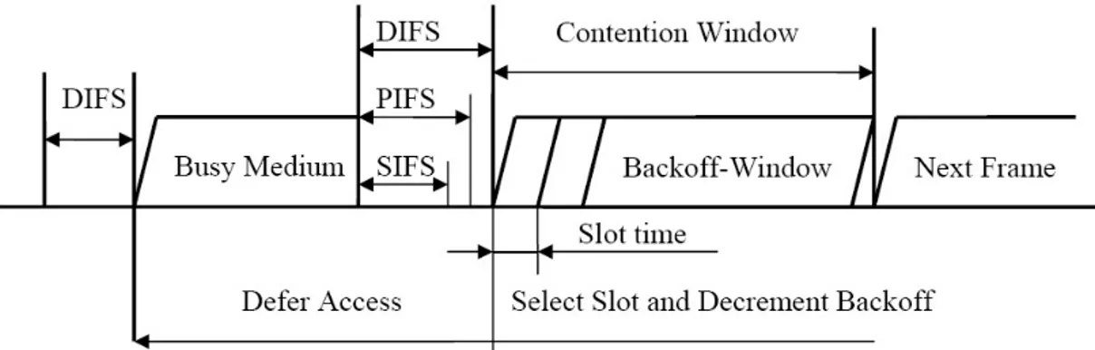
Before a station can send a data frame, it must sense the status of the medium. If the medium is busy, the station has to wait for the end of the current transmission followed by a defined interframe space (IFS) and a further randomly calculated backoff interval (cf. figure 2.3). Afterwards, it has to check again whether the medium has become busy in the meantime. If not, it starts to transmit.

The appropriate IFS must be used according to the type of data that should be sent. For administrative frames such as acknowledgements, the shortest waiting period termed Short IFS (SIFS) is applied. Most data traffic demands the DCF IFS (DIFS) which is

(20)

slightly longer than the SIFS. Additionally, a PCF IFS (PIFS) and an Extended IFS (EIFS) are defined.

2.2.2 Carrier Sense Mechanisms

To determine the status of the medium two carrier sense mechanisms are implemented: the physical carrier sense performed by listening to the air interface and the virtual carrier sense based on medium reservation information. Only if both mechanisms report the medium to be free, it is considered to be unoccupied.

Virtual carrier sense is established by a so-called Network Allocation Vector (NAV) which predicts the future usage of the medium. The duration information of how long the medium will be busy is either announced in every MAC-header, or the medium is reserved for transmission by using RTS/CTS. This technique sends out a Request To Send (RTS) frame to reserve the medium for a given time, and the receiving station replies with a Clear To Send (CTS) to acknowledge this reservation. Every other station in range using the same wireless channel will then consider the medium to be occupied, regardless if it received only the RTS, the CTS, or both. This is done to avoid the hidden station problem.

As RTS/CTS introduces overhead to a transmission, it is only activated for frames ex-ceeding a configurable size (RTS Threshold ), although in most circumstances RTS/CTS is simply switched off.

(21)

2.3. Physical Boundaries 7

2.2.3 Acknowledgement and Fragmentation

A station has to respond with an acknowledgement (ACK) for each correctly received data frame. If the sender does not get the ACK in time, it retransmits the data frame. It cannot be determined if the data frame got lost on its way to the receiver or the ACK frame got lost on its way back to the sender.

Furthermore, fragmentation can be enabled to force a station to divide frames exceeding a configurable limit (Fragmentation Threshold ) into one or several sub-frames. As each of these fragments is acknowledged and – on demand – retransmitted separately, overall throughput on a highly error-prone transmission line can be increased.

Similar to the RTS/CTS mechanism, fragmentation is mostly not used.

2.3 Physical Boundaries

When dealing with wireless networks, one shall always be aware of the unpredictable nature of radio transmissions.

The most often used parameters to describe the quality of a radio link are the signal strength (SS) and the signal-to-noise ratio (SNR), which in the first instance depend on the output power of the sending station, the linearity of the amplifiers of both, sender and receiver, the polarization of the radio waves, and the type of antennae in use. It is obvious that a higher output power yields a higher signal strength. But this does not automatically lead to a better reception, because amplifiers introduce distortion if they are operated out of their ideal working point. This harmonic distortion can happen on the sending as well as on the receiving side.

Furthermore, the antenna has a big influence on the signal strength. It is characterized by its type and its antenna gain. And the alignment of the antenna is responsible for the polarization of the radio waves.

In addition to these predictable parameters the SS and the SNR are influenced by the environment. Interferences can occur due to other senders on the same or adjacent

(22)

frequency bands (e.g. other wireless networks, Bluetooth devices, microwave ovens,. . . ) and obstacles reflecting, refracting, or absorbing the radio signal.

Another important indicator of the link quality is the bit error rate (BER), which itself is dependent on the SS, the SNR, and the type of modulation in use.

It therefore can be stated that a wireless channel is far from being reliable and pre-dictable, as it is influenced by so many factors of its environment. And although a lot of simulations of wireless networks are done, they are often based on simplifying assumptions far away from reality [11]. This is even more astonishing as already the original IEEE 802.11 standard written in 1997 states [13, p. 9]:

The physical layers used in IEEE 802.11 are fundamentally different from wired media. Thus IEEE 802.11 PHYs3

• Use a medium that has neither absolute nor readily observable bound-aries outside of which stations with conformant PHY transceivers are known to be unable to receive network frames.

• Are unprotected from outside signals.

• Communicate over a medium significantly less reliable than wired PHYs.

• Have dynamic topologies.

• Lack full connectivity, and therefore the assumption normally made that every STA4 _{can hear every other STA is invalid (i.e., STAs may}

be “hidden” from each other).

• Have time-varying and asymmetric propagation properties.

3_{Physical Layers} 4_Station

(23)

3 Wireless Multi-Hop Networks

Today, most common mobile communication systems in fact rely on wired infrastruc-ture. GSM networks for instance require an existing SS7-based telephone network. The same is true for WLAN installations which in nearly all cases provide access to an intranet or the Internet for a mobile user. So the actual mobility only exists for the last hop to connect a wireless station to the routed, wired network.

The Single-Hop Network is therefore the typical usage scenario in a Wireless LAN, and the medium access protocol is solely focused on this mode of operation. Nevertheless, it is possible to forward packets over several nodes in a WLAN, thus creating a Wireless Multi-Hop Network. To make this work the network has to be run in ad hoc mode, in which communication can take place without the need of a central controlling station. In this chapter two approaches towards establishing a Wireless Multi-Hop Network are presented. Additionally, a short introduction to routing protocols for MANETs is given.

3.1 Multi-Hop Networks using One Channel

Most WMNs and MANETs are based on a Multi-Hop Network sharing a single radio channel. The main advantage of this mode of operation is that existing standard wireless hardware (like the routers of our testbed, see chapter 4.1.1) can be used and that routing protocols do not have to deal with the radio channel configuration. A

(24)

10 3. Wireless Multi-Hop Networks

drawback on the other hand is of course the decrease of overall throughput when adding new stations within one cell.

In figure 3.1 it can be seen that the interference range of a single node (node 4) is much larger then the actual transmission range, which means that although the data transmission of node 4 can only be receipt by nodes 3 and 5, the channel is also blocked for their neighbours (nodes 2 and 6). And this is only an ideal theoretical case, where all nodes are arranged in one line and placed at such a distance that they can only receive the signal of their direct neighbours! In reality even with this configuration it is possible that a central node is better heard from a farther away placed device than from a nearby one (cf. [11]). So it can be stated that it is not predictable how many nodes are interfering with each other, thus forming one single cell.

1 2 3 4 5 6 nc Re e r e a f r n e g t e n I sion s i R m a s n n g a _e r T

Figure 3.1: Transmission and Interference Range of a Single Channel WMHN Still sticking to the example of routing the traffic along a line, the throughput is expected to decrease with each added hop due to the occupation of the medium. Within a single cell (i.e., the region where the medium has to be shared and no spatial channel reuse is possible) the overall throughput in theory is _#links1 . The latency on the other hand increases per hop, since each router introduces delay because of routing and medium access.

This behaviour is only true for the ideal case that one single data stream is utilizing the network, as could be proofed by real-life experiments described in [15] and our measurements (see chapter 6). When it comes to concurrent data flows in the Multi-Hop Network, the medium access is unfair and does not divide the free bandwidth equally among the participating stations [16].

(25)

3.2. Multi-Hop Networks using Several Channels 11

One solution to address these performance problems is to reduce co-channel interference by using more than one frequency range for the radio links.

3.2 Multi-Hop Networks using Several Channels

Since throughput and latency dramatically suffer from using a single shared medium, the utilization of several radio frequency ranges is a logical consequence. The advantage is that more than one node within the single channel interference range can transmit at the same time, as shown in figure 3.2.

1

2

3

4

TX RX TX RX TX RX

Channel A Channel B Channel C

Figure 3.2: Simultaneous Transmissions on a Multi Channel WMHN

For this model to work in an ideal way, channels have to be assigned carefully, which means that neighbouring links must preserve a certain distance in the frequency band to each other to reduce co-channel interference [17], and that spatial channel reuse is possible without disturbing other links.

One possibility to achieve this goal is manual frequency planning, as it is done for cellular networks (e.g. GSM, UMTS,. . . ) [18]. Another way is to use a routing pro-tocol and additionally modify the MAC-layer [19] or implement a software [20] that automatically assigns channels to wireless links.

The biggest drawback for using several channels is the need of more than one radio transceiver per node, thus increasing hardware complexity and costs. Also errors are harder to be spotted, since all utilized frequency bands must be surveyed. And finally, the frequency range for Wireless LANs is finite, so using up all available channels does not leave interference-free place for other wireless networks in the neighbourhood.

(26)

3.3 Routing Protocols for Wireless Mesh Networks

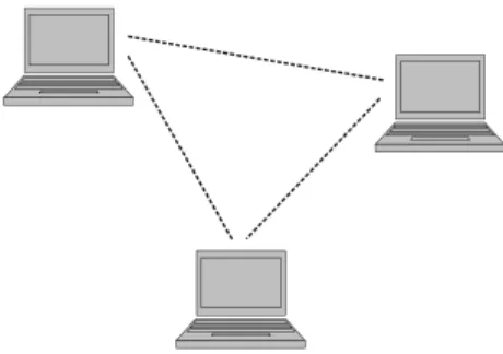
A Wireless Mesh Network is formed of interconnecting several multi-hopable nodes, as shown in figure 3.3. It relies on specialized routing protocols, which automatically adapt to topology changes and therefore also make mobility possible.

Figure 3.3: Wireless Mesh Network

Routing protocols in general are in charge of finding and establishing the ideal way for a packet to its destination. A routing protocol for a Wireless Mesh Network furthermore has to be aware of the different nature of radio links, e.g. that only devices inside a certain range are connected to each other. It needs to address the following issues:

• The routing tables have to be always up-to-date. If nodes die, move or arouse, the tables have to be immediately updated.

• The convergence of routing protocols should only use a small amount of messages and time.

• A node has to choose the most appropriate route for the packet. This can be the fastest, most reliable, highest throughput, or cheapest route.

• The routing table for each node has to stay as small as possible.

Currently, over 70 routing protocols for WMNs and MANETs are available. A contin-uously updated list of them can be found in [21].

In general, the route finding process for all protocols is similar: At first a new station that wants to take part in the mesh network does not know about its neighbours and

(27)

3.3. Routing Protocols for Wireless Mesh Networks 13

the network topology. So it has to introduce itself to the network and to listen to messages of other nodes within its receiving range. After it has learned routes from its neighbours, it also starts to broadcast routing information to all nodes within its transmission range.

Nowadays, two big groups of routing protocols for WMNs and MANETs are existing, which are going to be introduced in the following subsections.

3.3.1 Reactive Protocols

As the name states reactive routing protocols establish a route as a reaction to a desired data transfer. They find a way on demand, what leads to a high initial latency for setting up a connection, since the delivery of the data packet must be deferred until the information about the ideal route has arrived.

The most prominent reactive protocol is AODV.

3.3.1.1 Ad hoc On-demand Distance Vector (AODV)

The Ad hoc On-demand Distance Vector (AODV) Routing Protocol (RFC 3561 [22]) is a reactive routing protocol which is based on the distance vector algorithm also used in RIP1_.

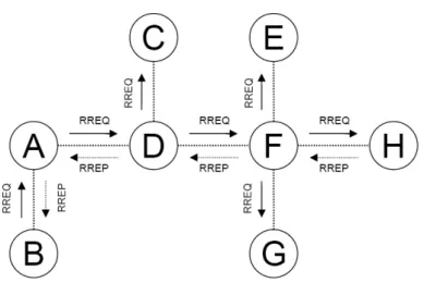
If a node wants to transmit data to a host of which it has no entry in its routing table, a route request (RREQ) is sent out. As can be seen in figure 3.4, all stations forward this message until the destination node (here: H) is reached. This node then unicasts a route reply (RREP) back to the origin of the message (here: B).

If an earlier station on the way already knows a path to the destination, it also replies with a RREP. The sender then chooses the route with the least number of hops. The nodes are checking the link status for active routes and report a link breakage with transmitting a route error message (RERR) to let other nodes know about the failure of a link. If routes become invalid or lost, AODV starts its route request again. To avoid huge routing tables, routes which are not used for some time are dropped.

(28)

Figure 3.4: Route Reply (RREP) and Route Request (RREQ) in AODV

One advantage of this routing protocol is that it does not need extra bandwidth to keep up paths which are already known. Furthermore, distance vector routing protocols need very low amounts of memory and calculation.

On the other hand AODV takes more time to establish a connection, and the com-munication to build up a new route creates a flood of control traffic overhead at one moment.

3.3.2 Proactive Protocols

In contrast to reactive protocols proactive routing protocols are active before any actual data transfer is happening. So routing information is spread prior to using the network. And proactive protocols keep information about the topology of the whole network. In order to maintain and update the topology information and the routing tables, routing information is flooded periodically to all stations. In case of an event (station dying, arousing, or moving) additional updates can be sent.

The advantage of a proactive protocol is the low delay in setting up a connection due to the fact that every node knows the whole network infrastructure a priori. But therefore a continuous amount of control traffic overhead has to be accepted.

(29)

3.3. Routing Protocols for Wireless Mesh Networks 15

3.3.2.1 Optimized Link State Routing Protocol (OLSR)

The Optimized Link State Routing (OLSR) Protocol (RFC 3626 [24]) is a proactive link state routing protocol. Similar to OSPF2 information is flooded continuously through the network so that every node has a view of the whole network topology.

Figure 3.5: MultiPoint Relaying in OLSR

As OLSR is used in wireless networks, broadcasting routing information can become a serious performance problem. To avoid this danger, the flooding behaviour is adapted to Wireless Multi-Hop Networks. This is established by optimizing the update mech-anism to preserve bandwidth. The specific technique used is called MultiPoint Relay-ing (MPR). MPR tries to avoid duplicate transmissions by selectRelay-ing nodes actRelay-ing as relays. To make this work, each node has to calculate its own set of relaying stations. The calculation is based on the fact that this node can reach the multi-point relays with a minimum hop count of two. As seen in figure 3.5, the relaying stations are represented by black dots. These nodes forward OLSR information originating in the centre to all their neighbours.

Although link-state updates are transmitted continuously, it was shown in [26] that the control traffic overhead of a proactive protocol is more predictable and that OLSR in fact generates less overhead in a large network.

The disadvantage of OLSR is its dependence on more calculations. It also has a higher memory usage than AODV, so better hardware is required.

(30)

(31)

4 Testing Environment

The testing environment consisted of six standard SOHO WLAN routers and two lap-tops running Linux which were used at three different locations to determine variations in performance and behaviour of a Wireless Multi-Hop Network.

The hardware, its configuration, and the test locations are presented in this chapter together with three network tools which were used to gather data like the round trip time and the throughput of each test setup.

4.1 Hardware

4.1.1 Routers

The measurements were done with Linksys WRT54GL wireless routers. They run Linux as their operating system and can therefore be re-configured by one’s needs. The routers are based on a Broadcom 5352 CPU running at 200 MHz, 4 MB of flash, and 16 MB of RAM. An 802.11g wireless NIC and a configurable 6-port switch are included in the CPU. One of the switch ports (port 5) is internally connected to the CPU, while the other ports (0–4) are available on RJ45-plugs on the backside of the router. The switch can be programmed to assign its ports to several VLANs, what in the standard configuration is used to distinguish between the WAN-port and the four LAN-ports. Furthermore, a bridge can be installed to join the wired and the wireless LAN.

(32)

18 4. Testing Environment

The OpenWRT-based Freifunk-firmware (Version 1.2.1 - English) [27] was installed on the routers, which is specially made for running OLSR-based Wireless Mesh Net-works. All unnecessary services (including OLSR) were shut down. Instead of a routing daemon static routes were set up to minimize disturbing effects by unwanted traffic.

4.1.2 Wireless Parameters

Wireless LAN hardware offers several parameter which can be configured to achieve the maximum possible performance.

Since the amount of tests would have increased dramatically if always the best possible configuration had been searched for, we decided to carry out the measurements with the default values shown in table 4.1.

Parameter Value

Fragmentation Threshold 2346 (disabled)

RTS Threshold1 _{2347 (disabled)}

CTS Protection Mode disabled

Frame Burst disabled

TX Power 28 mW

Table 4.1: Wireless Parameters used for the Measurements

4.1.3 Computers

The tests themselves were carried out between two laptops running Linux (Backtrack SLAX Linux Distribution Beta 05022006; Kernel 2.6.12.2) [30]. Their hardware config-uration is shown in table 4.2, and the computers were always connected via Ethernet to the routers. Therefore the integrated wireless cards of the PCs have never been used in order to minimize measurement errors due to different antenna gains or wireless hardware.

1_{Although simulations of Natkaniec and Pach [28] show the advantage of using RTS/CTS in}

WMHNs, we did not use this mode, since performance problems without RTS/CTS protection mainly occur on highly loaded networks. The overall throughput of a Multi-Hop Network is in any case lower than the one of a Single-Hop Network, regardless of the RTS Threshold value [29].

(33)

4.2. Locations 19

Laptop A Laptop B

Model Acer Travelmate 8102WLMI Asus M6800N

CPU Intel Pentium M 740 @ 1.73 GHz Intel Pentium M 705 @ 1.5 GHz

RAM 512 MB DDR2 533 1280 MB DDR 333

LAN-Card Broadcom NetLink Gigabit Broadcom NetLink Gigabit

WLAN-Card Intel PRO/Wireless 2915ABG Intel PRO/Wireless 2100

Table 4.2: Hardware Specifications of the Laptops

4.2 Locations

As already mentioned in chapter 2.3 wireless links are highly influenced by their sur-rounding environment. So the goal for performing the tests was to find a nearly “static” place with no obstacles in the line of sight of the two routers, as few as possible moving objects (e.g. cars, people,. . . ), and no interfering wireless networks in the neighbour-hood.

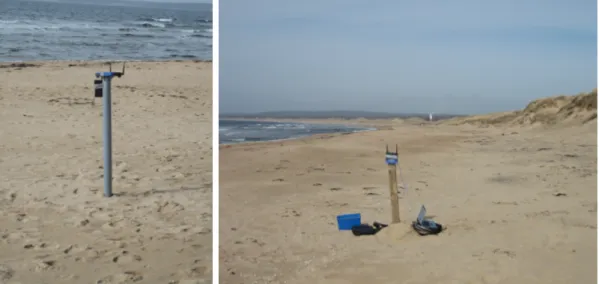
Being aware that there is no perfectly ideal location, the outdoor tests were done at the seaside. The beach of Tyl¨osand was separated from the residential area by sand hills and offered long open distances for the multi-hop tests. The hills were about 3 m high and 50 m away from the sea, with the actual sandy beach being flat and obstacle-free. At the testing location no other wireless network could be detected2_.

As shown in figure 4.1 the routers were placed on PVC or wood poles at a height of 1 m and a distance of 100 m each. Power supply was established using 14 V/7.4 Ah motorbike rechargeable batteries.

A second test series was made in an indoor environment. The routers were placed on office desks (height: 72 cm) in one line with a distance of 1 m each. Typical for a residential area the WLAN radio band was fully utilized by having interfering networks on channels 1, 6, and 11 in the neighbourhood.

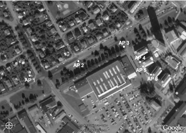
The third test scenario was built up in an urban environment, where a radio link between a house and the university was installed. As seen in figure 4.2, six routers were placed to create an 802.11g connection. The focus was set on being able to establish the link with the highest speed possible (54 MBit/s) on cost of the distance

(34)

Figure 4.1: Testing Location at the Beach of Tyl¨osand

between the routers. The map shows the position of the nodes represented by white dots. The grey dots show interfering wireless networks in the neighbourhood of the test setup3_{. Detailed information about the distance between the routers and their}

environment can be found in table 4.3.

4.3 Software

The set up Multi-Hop Networks were tested with several programs which were chosen to meet the following requirements:

• Measure the maximum possible throughput of reliable (TCP) and non-reliable (UDP) packet delivery

• Determine the introduced delay depending on varying packet sizes

• Show a relation between the size of sent data blocks to the actual throughput and latency on a reliable (TCP) connection

All three points were addressed by the software described below.

(35)

4.3. Software 21

Figure 4.2: Map of the Wireless Test Setup in an Urban Environment

Link Distance Environment

AP 1–2 125 m Direct sight, outside, AP 1 on balcony

AP 2–3 121 m Direct sight, outside, AP 2 on 1 m, AP 3 on 2 m height

AP 3–4 55 m Direct sight, outside, AP 4 on 5th floor (20 m height)

AP 4–5 15 m Indoor on same floor, separated by a wall

AP 5–6 30 m Direct sight, same height, window to window

AP 1–6 305 m Line of sight distance

AP 1–6 346 m Shortest way via each hop

(36)

4.3.1 Ping

Ping [32], coded by Mike Muuss in 1983, is a network tool testing the reachability of a certain host within an IP network. It sends out ICMP echo requests (type 8, code 0) to which the receiving host shall answer with according ICMP echo replies (type 0, code 0).

A

B

T T R T T R

..

.

l a vr et nI t u o e mi T Seq=1 Seq=10 Seq=11 Seq=2 1 = q e S 2 = q e S 1 1 = q e S

Figure 4.3: Sequence Diagram of PING

As seen in figure 4.3 every outgoing packet is stamped with a sequence number to associate it with its incoming response. Besides the IP and ICMP header, data can be attached to test the behaviour of IP packets with varying size.

The ping utility then measures the time it takes for each packet to receive the ac-cording answer. This is called the round trip time (RTT) and mostly depends on the latency of the transmission channel, the networking hardware (switches, routers, sending/receiving hosts), and the packet size.

ICMP packets are transmitted at a constant interval (default 1 s). If the response is not received within the doubled time of the average RTT, the packet is considered to be lost (cf. sequence 10 of figure 4.3).

Ping finally prints out the packet loss rate and further statistics of the measurements, namely the minimum, the average, the maximum, and the median deviation of all received packets.

(37)

4.3. Software 23

4.3.2 Iperf

For bandwidth measurements the open source tool Iperf (version 2.0.2) [33] was used. Iperf either transmits UDP datagrams at a specific sending rate to measure the actual received speed, the packet loss, and the jitter or TCP streams with a configurable windowsize to evaluate the maximum reliable throughput.

The program itself is both, sender and receiver. On one host it has to be started as the server to which another instance of Iperf (the client) connects and transmits data. Finally, the server displays the results and sends them to the client.

4.3.3 NetPIPE

Similar to the measurements described in [34] the Network Protocol Independent Per-formance Evaluator (NetPIPE) [35] version 3.6.2 was used to visualize the relation of the size of the sent blocks to the TCP throughput and the introduced latency on the links.

Like Iperf this tool is started as a server on one node to which the client instance connects. It then sends data blocks of increasing size and measures the RTT until it exceeds one second. For each blocksize three measurements are taken: one with the blocksize itself and two with the blocksize increased/decreased by a perturbation factor with a default value of 3. This is done in order to figure out block sizes which are slightly higher or smaller than an internal network buffer. Each test of each blocksize is repeated several times (default: 10) of which the smallest RTT is taken.

The blocksize, the throughput in MBit/s, and the RTT in seconds are recorded to a file.

(38)

(39)

5 Measurements

In this chapter the carried out measurements are introduced.

At first a test sequence is defined which was run for most of the further described tests. Then, before beginning the actual work, reference tests were done to verify if the chosen hardware was suitable for measuring. Therefore performance analyses were made for the computers and the routers on a wired network, which were afterwards compared to results of a wireless reference test. To provide a comparable base for the performance data of the Wireless Multi-Hop Networks, also wired multi-hopping was evaluated. Finally, the wireless test scenarios are outlined, with their results being discussed in chapter 6.

5.1 Test Sequence

For carrying out the measurements, a fixed test sequence was defined. It consisted of four individual tests:

• PING Test

• Maximum TCP Throughput Test (Iperf TCP) • UDP Test (Iperf UDP)

• NetPIPE Test

(40)

26 5. Measurements

For the PING Test 10 round trip times were taken of each of the following packet sizes: 64 Byte, 512 Byte, 1 kB, 4 kB, 16 kB, and 32 kB. Afterwards, 100 RTTs were measured for the packet size of 64 Byte.

The maximum TCP Throughput Test as well as the UDP Test were carried out with Iperf. The default values for sending (16 kB) and receiving (85.3 kB) window on TCP and sending (109 kB) and receiving (109 kB) buffer on UDP were kept, the UDP datagram size being static at 1470 Byte.

For the UDP Test various sending rates (100 kBit/s, 250 kBit/s, 500 kBit/s, 1 MBit/s, 2 MBit/s, 4 MBit/s, 8 MBit/s, 16 MBit/s, and 32 MBit/s) were tested and the received bandwidth, the packet loss, and the jitter recorded.

Finally, NetPIPE was used to measure throughput and latency of data blocks with increasing size. Here, the defaults of a perturbation factor of 3 and ten testing sequences per blocksize were kept, and the connection was reset after each individual test.

5.2 Reference Tests

Prior to the actual wireless multi-hop tests reference values were measured to get an understanding of the maximum performance of the hardware and the wireless channel.

5.2.1 Hardware Tests

Initially, the laptops as well as the routers were tested to prove that the used hardware was able to handle the generated traffic. Therefore a pure wired network was set up, in which the PCs were at first directly connected to each other and later plugged to a WRT in switching and finally in routing mode.

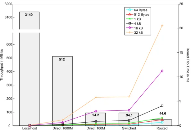
The results in figure 5.1 show that the PCs are able to handle TCP streams of up to several GBit/s on the localhost and 512 MBit/s via their network interfaces in Gigabit Ethernet mode. Even the integrated switch of the WRT54GL manages to establish a data rate similar to a direct Fast Ethernet connection.

(41)

5.2. Reference Tests 27

Localhost Direct 1000M Direct 100M Switched Routed 0 100 200 300 400 500 600 3100 3200 Throughput in MBit/s 0 5 10 15 20 25

Round Trip Time in ms

64 Bytes 512 Bytes 1 kB 4 kB 16 kB 32 kB 3140 512 94.2 94.1 44.6

Figure 5.1: Maximum TCP Throughput vs. Median RTT of the Hardware Only when it comes to routing, the limits of the used hardware are recognizable, as packet forwarding is purely done in software (i.e., via the CPU) on the WRTs. The impact of this is also observable for the highly increased latency, given by the median of 10 ICMP sequences with varying packet size.

5.2.2 Multi-Hop Tests

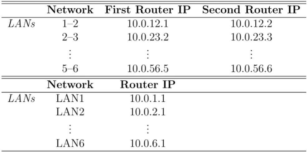
A second test series was carried out to evaluate the influence of additional hops on throughput and latency. For this up to six WRTs in routing mode were connected to each other via cable (cf. figure 5.2). The corresponding network configuration is listed in table 5.1.

Figure 5.3 visualizes the result of the NetPIPE test of this Wired Multi-Hop Network. The figure consists of three different diagrams.

The first diagram is called the network throughput graph and shows the relation of the sent blocksize to the throughput. It can be seen that the throughput increases with a

(42)

28 5. Measurements

1 PC A

PC B

2

3

4

5

6

2-3 1 -2 5-6 3 -4 4-5

LAN1 LAN4 LAN5

LAN2 LAN3 LAN6

Figure 5.2: Network Topology of the LAN Reference Tests

Network First Router IP Second Router IP

LANs 1–2 10.0.12.1 10.0.12.2 2–3 10.0.23.2 10.0.23.3 .. . ... ... 5–6 10.0.56.5 10.0.56.6 Network Router IP LANs LAN1 10.0.1.1 LAN2 10.0.2.1 .. . ... LAN6 10.0.6.1

(43)

5.2. Reference Tests 29 10 100 1,000 10,000 100,000 1,000,000 0 10 20 30 40 50 Blocksize in Byte Throughput in MBit/s 1 10 100 1,000 0 10 20 30 40 50

Throughput in MBit/s 1 10 100 1,000 1 100 10,000 1,000,000

Blocksize in Byte

1 Router 2 Routers 3 Routers 4 Routers 5 Routers

1 2 3 4 5 1 2 3 4 5 1 2 3 4 5

(44)

30 5. Measurements

higher blocksize. This is due to a better utilization of the link layer frames and a lower ratio of overhead compared to user data. Of course, the network is fully utilized at a certain point and cannot achieve even higher throughput then.

It is clear that sending larger blocks leads to higher latency. This is observable in the second diagram, the network signature graph. Here the throughput is compared to the round trip time.

The network saturation graph in the bottom of the figure finally shows the blocksize versus the round trip time. At a specific size of the messages the throughput is at its maximum. Any further enlargement of the sent blocks only increases the latency, denoted by a linear increase of the graph (compared to the non-linear gain before). From this point on the network is said to be saturated, hence the name saturation point.

If the three graphs are compared to each other with respect to the number of routers, one can see that the network behaves similar in all six cases. However, the overall performance in the multi-hop case is affected by a steady decrease of throughput ac-companied by an increase of latency when adding further routers.

This is also obvious for the comparison of the saturation points of the one router network with the six router network. While the network is saturated with 38 MBit/s at a blocksize of 20,000 Byte in the single router setup, a six router network only reaches saturation with a throughput of 30 MBit/s and a blocksize of 100,000 Byte. Because of the five times larger blocks also the round trip time speeds up from about 5 ms for the one hop to about 25 ms for the six hop setup.

This performance behaviour can more clearly be seen in figure 5.4 showing that on the Wired Multi-Hop Network the maximum TCP throughput decreases linearly by ap-proximated 1.11 MBit/s per router. At the same time the introduced delay increases by 0.47 ms for the median values of 100 ICMP packets with 64 kB in size. A strong correlation between the number of hops and the performance loss is proven by correla-tion factors of 99.82 % and 99.95 % to their regression lines for throughput and RTT respectively.

(45)

5.2. Reference Tests 31 1 2 3 4 5 6 38 39 40 41 42 43 44 45 Number of Routers Throughput in MBit/s 0.5 1 1.5 2 2.5 3

Median RTT Maximum TCP Throughput

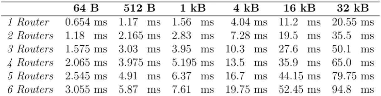
Figure 5.4: TCP Throughput and Median RTT depending on the Number of Routers The linearity of the RTTs is not surprising, because the total delay consists of the latency of the two PCs, the propagation delay of the links, and the routing delay. The propagation speed on a Twisted Pair cable is 177,000 km/s leading to a delay of approximately 5.65 ns on a 1 m Ethernet cable. It is therefore negligible. Furthermore, the number of PCs remains constant during all tests so that the introduced delay is mainly related to the routing processes of the WRTs. Therefore the latency grows linearly with the number of added routers, as already proven and shown in figure 5.4. Additionally, the median round trip times for varying packet sizes are listed in table 5.2.

64 B 512 B 1 kB 4 kB 16 kB 32 kB 1 Router 0.654 ms 1.17 ms 1.56 ms 4.04 ms 11.2 ms 20.55 ms 2 Routers 1.18 ms 2.165 ms 2.83 ms 7.28 ms 19.5 ms 35.5 ms 3 Routers 1.575 ms 3.03 ms 3.95 ms 10.3 ms 27.6 ms 50.1 ms 4 Routers 2.065 ms 3.975 ms 5.195 ms 13.5 ms 35.9 ms 65.0 ms 5 Routers 2.545 ms 4.91 ms 6.37 ms 16.7 ms 44.15 ms 79.75 ms 6 Routers 3.055 ms 5.87 ms 7.61 ms 19.75 ms 52.45 ms 94.8 ms

(46)

32 5. Measurements

5.2.3 Wireless Tests

The performance of a wireless network was measured in the already introduced indoor environment. For this purpose the routers were at first set up as Wireless Ethernet Bridges to acquire the maximum throughput possible in the wireless domain. Then the final test configuration, as it is going to be introduced in section 5.3.1, was established for one wireless link, and the performance was compared.

Bridging is a special mode of operation that has to be activated on one of the two routers, while the other one is acting as an access point. This managed mode must be taken if LAN and WLAN are bridged, because the performance suffers fatally as soon as the routers are run in ad hoc mode. We assume, this is due to broadcast packets bouncing between the two routers1_.

As can be seen in figure 5.5 the maximum wireless speed between two routers is far from the throughput the same routers are able to transport via cable, regardless of the wireless link layer speed and the mode of operation (bridged/routed). Furthermore it is obvious that the impact on the throughput of configuring the routers to ad hoc mode and enabling routing between wired and wireless network is significant. This performance loss is emphasized by the median latency values given in table 5.3.

5.2.4 Conclusion

It can be shown that the laptops and the routers are fast enough to handle throughput higher than the maximum possible speed of an 802.11g network. Although letting the devices route the traffic obviously has an impact on the performance, this does not limit the throughput at an upper bound, since the loss of maximum throughput affects both, high and low link-layer data rates. Similarly the latency increases due to the routing process at all link-layer speeds.

1_{A broadcast packet (e.g. ARP request) is sent on LAN A to router A bridging this packet to}

the WLAN. Router B receives the packet, forwards it to LAN B and rebroadcasts it on the WLAN. Router A again gets the message and broadcasts similar to router B. The packet is now bouncing between the two stations.

(47)

5.2. Reference Tests 33

LAN Routed WLAN Bridged WLAN Routed

0 5 10 15 20 25 30 35 40 45 50 Throughput in MBit/s 100M 54M 36M 18M Adaptive 43.2 23.1 18.3 11.3 18.8 17.6 15.2 10.3 17.6

Figure 5.5: Maximum TCP Throughput of Two Routers on LAN and WLAN

64 B 512 B 1 kB 4 kB 16 kB 32 kB LAN Routed 2 Routers 1.18 ms 2.165 ms 2.83 ms 7.28 ms 19.5 ms 35.5 ms WLAN Bridged 18 M 1.03 ms 1.825 ms 2.685 ms 6.41 ms 21.75 ms 40.45 ms 36 M 0.972 ms 1.56 ms 2.16 ms 4.43 ms 12.59 ms 25.15 ms 54 M 0.926 ms 1.48 ms 2.0 ms 3.85 ms 11.7 ms 20.15 ms Adaptive 0.994 ms 1.495 ms 2.07 ms 4.285 ms 13.05 ms 23.95 ms WLAN Routed 18 M 1.64 ms 2.63 ms 3.505 ms 11.05 ms 38.7 ms 72.4 ms 36 M 1.62 ms 2.4 ms 3.015 ms 9.29 ms 30.2 ms 57.0 ms 54 M 1.565 ms 2.285 ms 2.84 ms 8.33 ms 27.45 ms 52.15 ms Adaptive 1.605 ms 2.31 ms 2.87 ms 8.57 ms 27.65 ms 51.75 ms

(48)

34 5. Measurements

5.3 Test Series

For the wireless multi-hop measurements the sequence described in section 5.1 was performed at fixed link-layer data rates of 18 MBit/s, 36 MBit/s, and 54 MBit/s in 802.11g-only mode and with automatic data rate adaption in 802.11b/g-compatible mode. Only in the urban environment the UDP tests were omitted.

5.3.1 Wireless Multi-Hop Tests using One Channel

At first, multi-hop tests on one channel were performed in the described 1 m-distance indoor as well as in the 100 m-distance outdoor environment.

All links were configured to be on separate networks so that the routers always had to process and forward the IP-packets. As the routers only had one wireless NIC, the physical interface was split up by software into two virtual interfaces serving two IP-networks. The interface configuration and the packet routing of router 2 can be seen in figure 5.6. LAN-Interface WLAN IP 1-2 WLAN IP 2-3 WLAN-Interface Routing IP LAN2

Figure 5.6: Two IP-Networks on a Single Shared Interface

All radio communication took place on channel 13 with a single SSID, and measure-ments were done using 1 to 5 wireless links indoors and 1 to 4 links outdoors. The network topology and IP configuration are shown in figure 5.7 and table 5.4.

(49)

5.3. Test Series 35

1 PC A

PC B

2

3

4

5

6

2-3 1 -2 5-6 3 -4 4-5

LAN1 LAN4 LAN5

LAN2 LAN3 LAN6

Figure 5.7: Network Topology for the Multi-Hop Tests using One Channel

WLANs 1–2 10.1.12.1 10.1.12.2 2–3 10.1.23.2 10.1.23.3 .. . ... ... 5–6 10.1.56.5 10.1.56.6 Network Router IP LANs LAN1 10.0.1.1 LAN2 10.0.2.1 .. . ... LAN6 10.0.6.1

(50)

36 5. Measurements

Similar to the wired multi-hop tests the total round trip time on the wireless link consists of the latency of the two PCs, the propagation delay of the links, and the routing delay. But here the propagation delay can be further split up into the delay of the wired links and the delay of the wireless links.

Like the number of PCs the number of Ethernet links remains constant and is therefore a static parameter. As furthermore the propagation speed of a radio link is the speed of light (299,792.5 km/s), the introduced delay on 1 m distance is negligible with 3.34 ns in the indoor environment. For the 100 m distance outdoor test on the other hand, the propagation delay grows to 0.3 ms and therefore affects the overall round trip time. However, the latency should grow linearly with the number of added routers, because with each router also a further wireless link is established.

5.3.2 Wireless Multi-Hop Tests using Several Channels

For the next measurements a Wireless Multi-Hop Network using several channels was built up in the indoor environment.

One station had to be represented by a pair of routers, because two wireless NICs were needed to configure two separate radio links. The router pair was connected via Ethernet, and similar to the first test series each link got its own IP-network (see figure 5.8 and table 5.5).

In order to establish a maximum distance in the frequency band, radio communication took place on channels 1 and 13 for the two links test and 1, 13, and 7 for the three links test. Each wireless link also operated with its own SSID.

At first, the two routers of one router pair were stacked and the pairs placed at 1 m distance of each other. Unfortunately, the performance results were even worse than in the single channel 4-links test, until the routers of each router pair were also separated by 1 m. Furthermore, the directions of the antennae had to be changed in a way that each link had its unique polarization (vertical, horizontal, and facing each other). We assume that this extreme performance drop was due to bad selectivity of the receivers.

(51)

5.3. Test Series 37

1 PC A

PC B

2

3

4

5

6

2-3 1 -2 5-6 3 -4 4-5 LAN1 LAN4 LAN6

Figure 5.8: Network Topology for the Multi-Hop Tests using Several Channels

WLAN - ch. 1 1–2 10.1.12.1 10.1.12.2 LAN 2–3 10.0.23.2 10.0.23.3 WLAN - ch. 13 3–4 10.1.34.3 10.1.34.4 LAN 4–5 10.0.45.4 10.0.45.5 WLAN - ch. 7 5–6 10.1.56.5 10.1.56.6 Network Router IP LANs LAN1 10.0.1.1 LAN4 10.0.4.1 LAN6 10.0.6.1

(52)

38 5. Measurements

Since for this test constellation two routers have to mimic one station with two wireless interfaces, the introduced delay does not grow linearly. For the two links setup the latency consists of the delay of the two PCs, three Ethernet links, and two wireless links, whereas for the three links setup the delay of two PCs, four Ethernet links, and three wireless links has to be calculated. It is hard to tell, which fraction of the overall delay is due to which link, so a discussion of the round trip times of this setup is omitted.

5.3.3 Wireless Multi-Hop Tests in Urban Environment

The last test series was set up similar to the multi-hop tests on one channel. Like in the first measurements channel 13 and a single SSID were used, and the IP-networks and interfaces were configured the same.

The difference to the first test series was on one hand the environment, introduced in section 4.2, and on the other hand the carried out tests. Instead of evaluating a varying number of wireless links, the maximum TCP throughput and the round trip times of each individual link were measured. Finally, the complete way from the house to the university was tested, and TCP throughput, PING, and NetPIPE results recorded.

(53)

6 Discussion of the Results

In this chapter the results and findings of the tests, which were introduced in the previous section, are presented and discussed.

Before the different environments are compared to each other, the influence of the link-layer speed of a wireless network is shown.

6.1 Throughput on a Single Wireless Link

The diagrams in figure 6.1 present the TCP throughput and latency performance for various link-layer speeds of a single link in the indoor environment. As expected, the highest possible throughput of all data rates is nearly the half if not less of the promised link-layer speeds.

In the figure it can clearly be seen that all of the different speeds behave similarly. This is most obvious for the network saturation graphs in the bottommost diagram, which superpose for all four measurements. The only difference is the maximum throughput limited by the given link-layer speed. The diagrams further imply that the adaptive rate mode uses 54 MBit/s, what is denoted by the superposition of the graphs of these two speeds.

Between the blocksize of 1,000 Byte and 1,500 Byte a slower gain in throughput is visible. Especially on the three highest link-layer speeds this looks like a “knee” which is also recognizable in the signature graph. This phenomenon is due to the Maximum Transfer Unit (MTU) of the Wireless LAN.

(54)

40 6. Discussion of the Results 10 100 1,000 10,000 100,000 1,000,000 0 5 10 15 20 Blocksize in Byte Throughput in MBit/s 1 10 100 1,000 0 5 10 15 20

Blocksize in Byte 18M 36M 54M Adaptive Adaptive 54M 36M _18M 18M 18M 36M 36M 54M 54M Adaptive Adaptive

(55)

6.2. The Influence of Multiple Hops on Throughput and Latency 41

If packets exceeding the MTU of the link layer are transported, they have to be split up into two or more link layer frames. This introduces higher overhead and therefore lowers the actual throughput.

Because the result shows that the behaviour of an 802.11g network in an indoor environ-ment is independent from the link-layer speed, further diagrams in an ideal environenviron-ment are focused on the 54 MBit/s mode.

6.2 The Influence of Multiple Hops on Throughput

and Latency

The presentation of the multi-hop measurements starts with a comparison of UDP and TCP in a Wireless Multi-Hop Network, which is followed by showing the impact of the number of wireless links on TCP throughput and ICMP round trip time. Finally, the behaviour of TCP streams with varying blocksizes is analysed.

6.2.1 Comparison of Maximum UDP and TCP Throughput

As it is widely known, the User Datagram Protocol (UDP) does not provide reliability and ordering guarantees. Therefore it is less complex and allows higher raw throughput than TCP. The maximum received bandwidth is obtained by transmitting a higher bandwidth than the network is able to carry. The quantity and rate of the nevertheless passing datagrams then leads to the presented raw UDP throughput.

Figure 6.2 compares the maximum throughput of the two protocols depending on the number of wireless links. The measurements prove that UDP tops TCP with about 33 % in raw throughput on one wireless link. The difference can be explained with the reliability aim of TCP which requests acknowledgements for each successfully transmit-ted sequence and retransmissions for corruptransmit-ted sequences. This overhead consequently eats up a part of the bandwidth. It furthermore blocks the medium, thus worsening the actual throughput on a half-duplex connection compared to a full-duplex link.

(56)

42 6. Discussion of the Results 1 2 3 4 0 5 10 15 20 25 Wireless Links Throughput in MBit/s UDP TCP 23.0 17.3 12.4 9.8 8.1 6.3 _6.0 4.6

Figure 6.2: UDP vs. TCP Throughput Depending on the Number of Links (54 MBit/s) Although the impact of several links on the throughput should affect the acknowledging TCP-stream more than the “one-way-only” UDP datagrams, this could not be verified. In fact, TCP seems to behave quite similar compared to UDP, even if more hops are added. So the UDP throughput for four links is still about 30 % higher than the TCP throughput. Possibly this effect is related to the MAC-layer acknowledgements, mentioned in section 2.2.3.

This finding led to the decision to furthermore concentrate on the results of the TCP tests, since also the UDP results of the jitter only showed unpredictable behaviour.

6.2.2 Maximum Throughput and Latency

As already shown in the last subsection, the number of links has a high impact on the maximum throughput of a Wireless Multi-Hop Network. To further underline this, table 6.1 lists the maximum TCP throughput for several link-layer speeds measured with Iperf.

(57)

6.2. The Influence of Multiple Hops on Throughput and Latency 43 Wireless Links 1 2 3 4 5 54M 17.6 9.55 6.46 4.65 3.64 MBit/s 36M 15.2 7.77 5.32 3.97 3.00 MBit/s 18M 10.3 5.23 3.43 2.46 1.92 MBit/s Adaptive 17.6 9.38 6.28 4.58 3.49 MBit/s

Table 6.1: Throughput with 18M, 36M, 54M and Adaptive Rate

That the throughput decreases with the number of wireless hops as _#links1 was already stated in chapter 3.1 and is clearly observable in figure 6.3. This figure visualizes the influence of multiple hops on the maximum TCP throughput and the round trip time. In the diagram the straight lines show the measured values which are approximated by the dotted regression curves.

For fitting the throughput regression graph to the measured data the model y = a · xb

is used. In this formula x represents the number of links, y the resulting throughput, and a and b are the parameters to be found. The maximum throughput of the model is then given by a, whereas the decrease parameter b should reach −1, if the theoretical model was true.

The data values used for finding the parameters are listed in table 6.2 which also shows the performance in relation to one single wireless link for 54 MBit/s in indoor environment. Table 6.3 then presents the calculated parameters for indoor and outdoor environment. They validate the theoretical model, since the found decrease parameters are approximately the expected −1.

Besides the influence on the throughput, the impact on the latency is also shown in figure 6.3. Similar to a pure wired network the median RTTs increase linearly with an additional number of hops. The corresponding correlation coefficients to the regression line are 99.99 % for both, indoor and outdoor environment.

(58)

44 6. Discussion of the Results 1 2 3 4 5 0 2 4 6 8 10 12 14 16 18

Number of Wireless Links

Throughput in MBit/s 1 1.5 2 2.5 3 3.5 4 4.5 5 5.5 6

Median RTT Maximum TCP Throughput

Figure 6.3: Impact of Multiple Hops on TCP Throughput and Median RTT

Wireless Links Throughput Performance

1 17.6 MBit/s 100.0 % = 1

2 9.55 MBit/s 54.26 % ≈ 1/2

3 6.46 MBit/s 36.70 % ≈ 1/3

4 4.65 MBit/s 26.42 % ≈ 1/4

5 3.64 MBit/s 20.68 % ≈ 1/5

Table 6.2: TCP Throughput depending on the Number of Links at 54 MBit/s

Maximum Throughput (a) Decrease Parameter (b)

Indoor 17.7 MBit/s -0.9372

Outdoor 16.9 MBit/s -0.9035

(59)

6.2. The Influence of Multiple Hops on Throughput and Latency 45

6.2.3 The Behaviour of a TCP Stream in a Wireless

Multi-Hop Network

The behaviour of a TCP stream in a Wireless Multi-Hop Network is visualized by the results of the NetPIPE test. The diagrams in figure 6.4 compare throughput and latency depending on the number of wireless links.

In general, it can be observed that TCP behaves similar with 1 to 5 wireless links and that only the maximum throughput is reduced. As it is seen in the throughput graph, the throughput grows fast until a blocksize of approximately 4,000 Byte, from which on the increase is very small. Only on the single link network the throughput continues to quickly rise to a blocksize of about 25,000 Byte.

Like in figure 6.1 the “MTU-knee” is present here. Especially the throughput graphs of 2 to 5 wireless links show that the throughput is stable if not slightly decreasing in the surroundings of the MTU. Also in the signature graph in the centre of figure 6.4 this phenomenon is visible. It furthermore reveals that the throughput is affected by this “knee” at a higher round trip time the higher the number of links is.

Obviously, the delay introduced by forwarding packets has a big impact on the round trip times. Similar to the wired network the graphs start at different RTT-values, what shows the influence of routing and the access to the shared medium. If a deeper look on the delay is taken, it can be seen that for one wireless link the delay was only 0.5 ms at the smallest blocksize, whereas the RTT at five wireless links was already 1.8 ms at the same blocksize.

Because of the increased latency, the saturation point is reached at a higher RTT the more wireless links are used. The saturation point for one wireless link resides at a RTT of approx. 2 ms, for two links at approx. 3 ms, for three links at approx. 4 ms, for four links at approx. 6 ms, and for five wireless links at approx. 8 ms. When these stated RTTs are exceeded, the throughput almost remains constant, and only the delay grows linearly with a higher blocksize. This is observable in the saturation graph on the bottom.

(60)

46 6. Discussion of the Results 10 100 1,000 10,000 100,000 1,000,000 0 5 10 15 20 Blocksize in Byte Throughput in MBit/s 1 10 100 1,000 0 5 10 15 20

Blocksize in Byte

1 Link 2 Links 3 Links 4 Links 5 Links

1 1 1 2 2 2 3 4 5 3 4 5 3 4 5

(61)

6.3. Indoor vs. Outdoor Environment 47

6.3 Indoor vs. Outdoor Environment

As described in the test setup in section 4.2, indoor and outdoor measurements were done to determine if the environment has an impact on the performance and the delay of a wireless link.

6.3.1 Impact of the Environment on the Throughput

In figure 6.5 the TCP throughput graphs of the indoor and outdoor tests are presented. The solid lines represent the wireless indoor links, the broken lines the results of the outdoor tests. If a deeper look on the wireless links is taken, it can be see that the outdoor throughput is about 1 MBit/s less for one wireless link and about 0.5 MBit/s less for two wireless links. This may be caused by a higher bit error rate in the outdoor environment, thus increasing the number of necessary retransmissions.

An astonishing fact reveals the comparison of indoor and outdoor environment for three and four links, where the results are hardly distinguishable. Table 6.4 even shows that the throughput is better outdoors than indoors. One reason for this behaviour could be that spatial frequency reuse was possible due to a higher signal attenuation in the outdoor environment.

6.3.2 Impact of the Environment on the Round Trip Time

In the two diagrams of figure 6.6 the results of the ping tests for various packet sizes are plotted. The x-axes represent the tests at different link-layer speeds and with increasing packet size, whereas the y-axes show the median round trip times.

As can be seen in the diagrams, the latency increases linearly by the number of wireless links in the indoor environment. This behaviour is observable for each of the tested packet sizes.

The results of the outdoor measurements are in general similar to the indoor tests. Only two wireless links seem to perform explicitly better outdoors. A reason for this behaviour could not be found.

Performance Measurements in Wireless 802: 11g Multi-Hop Networks

MASTER’S THESIS