Distributed thermal response tests: New insights on U-pipe and Coaxial heat exchangers in groundwater-filled boreholes

(1)

Distributed thermal response

tests – New insights on U-pipe

and Coaxial heat exchangers in

groundwater-ﬁ lled boreholes

J O S É A C U Ñ A

Doctoral Thesis in Energy Technology

Stockholm, Sweden 2013

(2)

Distributed thermal response tests –

New insights on U-pipe and Coaxial

heat exchangers in groundwater-filled

boreholes

José Acuña

Doctoral Thesis 2013

KTH School of Industrial Engineering and Management Division of Applied Thermodynamics and Refrigeration

(3)

Trita REFR Report 13/01 ISSN 1102-0245

ISRN KTH/REFR/13/01-SE ISBN 978-91-7501-626-9 © José Acuña

(4)

Preface

A substantial amount of new insights about the operation and thermal response testing of U-pipe and Coaxial heat exchangers installed in groundwater filled boreholes are revealed in this experimental thesis work. I feel that I just planted one more seed to lots of further research to be done with the measurements presented here, but I can proudly say that ground source cooling and heating systems can be improved if the methods demonstrated in this thesis are implemented on existing and/or new installations.

This achievement is not only mine and it is hard to see how much work there is behind the measurements presented here. I would like to ac-knowledge those who helped me on this journey:

The first credit goes to the Swedish Energy Agency for financing this project through the EFFSYS+ and EFFSYS2 programs. This would have been impossible without our sponsors: Alfa-Laval, Ahlsell, Aska rör, AVANTI, Brage Broberg, Brunata, COMSOL, COOLY, Cupori, Ekofektiv, Energi-Montage, ETM Kylteknik, Extena, Geosigma, GRUNDFOS, Hydroresearch, Högalids elektriska, IVT, LAFOR Ener-gientrepenader, LOWTE, Lämpöässä, Mateve Oy, Merinova, GEOTEC, MuoviTech, Neoenergy, NIBE, Nowab, PEMTEC, PMAB, Prof. Rich-ard Beier, SEEC, Stures Brunnsborrningar, SUST, SVEP, SWECO, THERMIA, Tibnor, Thoren VP, Tommy Nilsson, UPONOR, Viess-mann, Willy’s cleantech, WILO. Thanks also to Prof. Eric Granryd, Erik Björk, Martin Forsén, and Anders Nilsson, and other members of the EFFSYS board, for coordinating these research programs.

Manil Bygg, Nordahl Fastigheter, Klas Andersson, Kenneth Weber, and JM, are specially acknowledged for kindly allowing us to carry out this research at their installations and for their support during this work. I would like to extend a very sincere gratitude to Tommy Nilsson who significantly helped to materialize many of these installations, and to Sam Johansson who introduced me to the fascinating world of distributed temperature measurements.

For their help during installations, I would also like to recognize the im-portant contributions of Peter Hill, Benny Sjöberg, Hans Alexandersson,

(5)

Karl-Åke Lundín, John Ljungqvist, Peter Platell, and Brage Broberg. I will always remember the magic phrase: AKTA fibern!

Thanks also to my dad José G. Acuña, to Michael Klasson, Åke Melinder, Erik Lindstein, Björn Kyrk, Mauri Lieskoski, Johan Wasberg, Jussi, Claudi, Samer, Bo Jansson, Jan Cederström, Willy Ociasson, Jan-Erik Nowacki, Rashid, Stina, Hatef, Carl, Julia, Jesus, Patricia, Tomas, Leoni, Maria, Andreas, Lukas, Tommy, Charles, Klaes, Eduard, Marcos, and Francois. You all gave me a hand at some point.

I would like to remember and acknowledge some people who no longer are physically with us but who helped and motivated me at different moments along this journey: Benny Andersson, Nabil Kasem, Olle Hellman, Stanisław (Sławek), Abuelo Sequera, and Abuela Carmen. A special recognition to my supervisor Prof. Björn Palm, whose hum-bleness and dedication inspired me day after day. Björn, thanks for trust-ing me, for your support and wise advices. Thanks also to you and Prof. Per Lundqvist for selecting me as a PhD student. I take the chance to greet our ETT family, it is a pleasure to be part of it! A special salutation to all my colleague PhD students for many moments together, especially to Monika and Hatef whom I had the pleasure to be roommate with. A very particular gratitude to Palne Mogensen, the pioneer of thermal re-sponse testing and the most precise person I have ever met. Thanks for teaching me among other things the secrets of TRTs, and for all your valuable critics. You are a professional role model to me. Thank you also for showing me a bit more of Sweden, a beautiful country that is now part of me.

Mamá, Papá, Abuela Mercedes, Maria, Miguel, Fatima, Eduardo, little princess Natalia, primos y tios, thanks for your support. I feel you often walk with me despite the distance that separates us!

And the most special credit goes to my beautiful wife, Dominika, for her infinite understanding, support and patience. This achievement is also yours! And to our daughters, Emilia and Amanda, for giving me even more reasons to finish this thesis. I love you!

It has been a fantastic journey thanks to all of you! May god give you health for many years to come!

Thank you!

(6)

Abstract

U-pipe Borehole Heat Exchangers (BHE) are widely used today in ground source heating and cooling systems in spite of their less than op-timal performance. This thesis provides a better understanding on the function of U-pipe BHEs and investigates alternative methods to reduce the temperature difference between the circulating fluid and the borehole wall, including one thermosyphon and three different types of coaxial BHEs.

Field tests are performed using distributed temperature measurements along U-pipe and coaxial heat exchangers installed in groundwater filled boreholes. The measurements are carried out during heat injection ther-mal response tests and during short heat extraction periods using heat pumps. Temperatures are measured inside the secondary fluid path, in the groundwater, and at the borehole wall. These type of temperature measurements were until now missing.

A new method for testing borehole heat exchangers, Distributed Ther-mal Response Test (DTRT), has been proposed and demonstrated in U-pipe, pipe-in-U-pipe, and multi-pipe BHE designs. The method allows the quantification of the BHE performance at a local level.

The operation of a U-pipe thermosyphon BHE consisting of an insulat-ed down-comer and a larger riser pipe using CO2 as a secondary fluid has been demonstrated in a groundwater filled borehole, 70 m deep. It was found that the CO2 may be sub-cooled at the bottom and that it flows upwards through the riser in liquid state until about 30 m depth, where it starts to evaporate.

Various power levels and different volumetric flow rates have been im-posed to the tested BHEs and used to calculate local ground thermal conductivities and thermal resistances. The local ground thermal conduc-tivities, preferably evaluated at thermal recovery conditions during DTRTs, were found to vary with depth. Local and effective borehole thermal resistances in most heat exchangers have been calculated, and their differences have been discussed in an effort to suggest better meth-ods for interpretation of data from field tests.

(7)

Large thermal shunt flow between down- and up-going flow channels was identified in all heat exchanger types, particularly at low volumetric flow rates, except in a multi-pipe BHE having an insulated central pipe where the thermal contact between down- and up-coming fluid was al-most eliminated.

At relatively high volumetric flow rates, U-pipe BHEs show a nearly even distribution of the heat transfer between the ground and the secon-dary fluid along the depth. The same applies to all coaxial BHEs as long as the flow travels downwards through the central pipe. In the opposite flow direction, an uneven power distribution was measured in multi-chamber and multi-pipe BHEs.

Pipe-in-pipe and multi-pipe coaxial heat exchangers show significantly lower local borehole resistances than U-pipes, ranging in average be-tween 0.015 and 0.040 Km/W. These heat exchangers can significantly decrease the temperature difference between the secondary fluid and the ground and may allow the use of plain water as secondary fluid, an alter-native to typical antifreeze aqueous solutions. The latter was demon-strated in a pipe-in-pipe BHE having an effective resistance of about 0.030 Km/W.

Forced convection in the groundwater achieved by injecting nitrogen bubbles was found to reduce the local thermal resistance in U-pipe BHEs by about 30% during heat injection conditions. The temperatures inside the groundwater are homogenized while injecting the N2, and no radial temperature gradients are then identified. The fluid to groundwater thermal resistance during forced convection was measured to be 0.036 Km/W. This resistance varied between this value and 0.072 Km/W ing natural convection conditions in the groundwater, being highest dur-ing heat pump operation at temperatures close to the water density maximum.

Keywords: Borehole Heat Exchangers, Distributed Thermal Response Test, Ground Source Heat Pumps, Coaxial, U-pipe, Multi-pipe, Pipe-in-pipe, Multi-chamber, Groundwater, Thermosyphon.

(8)

Nomenclature

α Thermal diffusivity of the surrounding ground [m2_/s]

∆T Temperature difference [K]

h Enthalpy [kJ/kg]

λ Thermal conductivity of secondary fluid [W/(m K)]

λrock Thermal conductivity of the surrounding ground [W/(m K)] λPE Thermal conductivity of polyethylene pipes [W/(m K)] mdot Mass flow rate of CO2 in thermosyphon BHE [kg/s]

Nu Nusselt number [-]

q’ Power per meter [W/m]

q1-12 Heat flow through the peripheral pipes in Multi-pipe BHE [W] q0 Heat flow through the central pipe in Multi-pipe BHE [W] qtotal Sum of heat flows through central and peripheral pipes [W]

Pr Prandtl number [-]

R Thermal resistance [Km/W]

Ran-bw Annulus-to-borehole wall thermal resistance [Km/W]

Rb Local borehole resistance [Km/W]

Rb* Effective borehole resistance [Km/W]

(9)

Rf-gw Secondary fluid-to-groundwater thermal resistance [Km/W] Rgw-bw Groundwater-to-borehole wall thermal resistance [Km/W]

Re Reynolds number [-]

Tamb Ambient temperature [°C]

Tan Secondary fluid temperature inside the annular flow channel [°C] Tbottom Fluid temperature at the bottom of a heat exchanger [°C]

Tbw Temperature of the borehole wall [°C]

Tbw mean Average borehole wall temperature vs. depth [°C] Tcp Secondary fluid temperature inside the central pipe [°C] Tin Temperature at the inlet of the borehole heat exchanger [°C]

Tf Secondary fluid temperature [°C]

Tgw Temperature of the groundwater [°C]

Tmean Average between inlet and outlet fluid temperature [°C] Tout Temperature at the outlet of a borehole heat exchanger [°C] Trock Temperature of the surrounding ground [°C]

ν Kinematic viscosity [m2_/s]

Note: The appended articles contain other symbols which are ex-plained in each specific paper

(10)

Str ucture of the thesis

Chapter 1 presents the general objective and gives a broad context to the subject of this research together with a brief explanation about the dis-tributed temperature measurement technique. Chapter 2 gives back-ground knowledge based on relevant previous work on borehole heat exchangers.

Chapters 3 to 7 aim at studying the specific objectives of this thesis, each on a particular borehole heat exchanger type. The specific objectives are presented at the beginning of each chapter, followed by a short summary of one published scientific paper (appended at the end of this thesis), as well as some new experiments and unpublished results. Each of the chapters presents individual conclusions based on the specific objectives set for the corresponding borehole heat exchanger type.

P u b l i c a t i o n s

The papers appended to this thesis are the following:

Paper I: J. Acuña, P. Mogensen, B. Palm. Distributed Thermal Response Test on a U-pipe Borehole Heat Exchanger. The 11th_{International} Con-ference on Energy Storage EFFSTOCK, Stockholm 2009.

Paper II: J. Acuña, B. Palm, R. Khodabandeh, K. Weber. Distributed Tem-perature Measurements on a U-pipe Thermosyphon Borehole Heat Ex-changer with CO2. 9th Gustav Lorentzen Conference. Sydney 2010. Paper III: J. Acuña, B. Palm. Distributed Thermal Response Tests on Pipe-in-Pipe Borehole Heat Exchangers. Accepted for publication. In press. Applied Energy, 2013.

Paper IV: J. Acuña, P. Mogensen, B. Palm. Evaluation of a Coaxial Bore-hole Heat Exchanger Prototype. 14th_{ASME IHTC International Heat} Transfer Conference, Washington D.C 2010.

Paper V: J. Acuña, P. Mogensen, B. Palm. Distributed thermal response tests on a multi-pipe coaxial borehole heat exchanger, HVAC&R Re-search, 17:6, 1012-1029. 2011.

(11)

Other publications by the author during the PhD studies but not in-cluded in this thesis are:

1. R. Beier, J. Acuña, P. Mogensen, B. Palm. 2013. Borehole resistance and vertical temperature profiles in coaxial borehole heat exchang-ers. Applied Energy 102 (2013), 665-675.

2. J. Acuña. Vatten som köldbärare i svenska bergvärmepumpar! Är det möjligt? KYLA Värmepumpar No 6 2012.

3. J. Acuña, M. Fossa, P. Monzó, B. Palm. Numerically Generated g-functions for Ground Coupled Heat Pump Applications. COMSOL Multiphysics Conference, Milano 2012.

4. E. Johansson, J. Acuña, B. Palm. Use of Comsol as a Tool in the Design of an Inclined Multiple Borehole Heat Exchanger. COM-SOL Multiphysics Conference, Milano 2012.

5. R. Beier J. Acuña, P. Mogensen, B. Palm. Vertical temperature pro-files and borehole resistance in a U-tube borehole heat exchanger, 2012. Geothermics 44 (2012), 23-32.

6. P. Monzó, J. Acuña, B. Palm. Analysis of the influence of the heat power rate variations in different phases of a DTRT. Innostock - The 12th_{International Conference on Energy Storage, Lleida, 2012.} 7. J. Acuña, B. Palm. Distributed Temperature Measurements on a

Multi-pipe Coaxial Borehole Heat Exchanger. The 10th_{IEA Heat} Pump Conference, Tokyo, 2011.

8. J. Acuña, B. Palm. First Experiences with Coaxial Borehole Heat Exchangers. IIR Conference on Sources/Sinks alternative to the outside Air for HPs and AC techniques, Padua, 2011.

9. J. Acuña. Framtidens värmesystem med borrhålsvärmeväxlare. Energi&Miljö nr 2 februari 2011.

10. J. Acuña, B. Palm. Comprehensive Summary of Borehole Heat Ex-changer Research at KTH. Conference on Sustainable Refrigeration and Heat Pump Technology, Stockholm, 2010.

11. J. Acuña. Effektivare Utnyttjande av Energibrunnar för Värmepum-par Undersöks på KTH. KYLA VärmepumVärmepum-par No 6 2010.

12. H. Madani, J. Acuña, J. Claesson, P. Lundqvist, B. Palm. The Ground Source Heat Pump: A System Analysis with a Particular Fo-cus on the U-pipe Borehole Heat Exchanger. 14th_{ASME IHTC} In-ternational Heat Transfer Conference, Washington D.C 2010. 13. J. Acuña, B. Palm. A Novel Coaxial Borehole Heat Exchanger:

De-scription and First Distributed Thermal Response Test Measure-ments. IGA World Geothermal Congress, Bali 2010.

14. J. Acuña. Optimera med rätt kollektorval. Borrsvängen nr. 2/2010. 15. J. Acuña, B. Palm. Local Heat Transfer in U-pipe Borehole Heat

(12)

16. J. Acuña. Efficient Use of Energy Wells for Heat Pumps. GeoCon-neXion Magazine. Canada, Fall 2009.

17. J. Acuña. Slang intill bergväggen ger effektivare värmeväxling. Hus-byggaren, nr 6 2009.

18. J. Acuña. Bergvärmepumpar Kan Göras Ännu Mer Effektiva, Ene-gi&Miljö no 3, 2008.

19. Hur bra kan ett borrhål bli? Interview. SVEP NYTT nr 3, 2008. 20. J. Acuña, B. Palm. Experimental Comparison of Four Borehole Heat

Exchangers. 8th_{IIR Gustav Lorentzen Conference, Copenhagen}

2008.

21. J. Acuña, B. Palm, P. Hill. Characterization of Boreholes: Results from a U-pipe Borehole Heat Exchanger Installation. 9th_{IEA Heat} Pump Conference, Zurich 2008. s4-p19.

Besides this, the author has during his PhD studies supervised 18 Master theses from the Energy Department at KTH and collaborated with the-sis supervision at Uppsala University, Karlstad University, Chalmers University of Technology, and University of Genoa.

Oral and poster presentations about this project have also been given by the author at seminars organized by Energi&Miljö Tekniska föreningen (EMTF), University of Genoa, Swedish Heat Pump association (SVEP), Kyltekniska Föreningen, Nordbygg 2008 and 2012, GeoEnergiTag 2011, the EU projects GEOPOWER and GroundMed, AVANTI, Swedish Energitinget 2009, GEOTEC, Geothermal PhD student day, University of Zagreb, EFFSYS2 and EFFSYS+ days, Sveriges energiting 2009, Nordic Climate Solutions conference 2008, Vasas energilösningar 2008 and 2009, Astech workshop Bilbao 2008, Exportrådet, and Näringslivets internationella råd.

Most publications and more information about this project can be found at http://www.energy.kth.se/energibrunnar, http://www.effsys2.se and

(13)

Figure 1. Illustration of the different types of coaxial BHE geometries 21 Figure 2. Mean fluid temperature variation with borehole resistance and specific heat extraction rates (calculated for one day of constant operation with λrock=2.5 W/mK, α=1.25x10-6 m2/s, and Trock=8°C) 27 Figure 3. Residence time of BHE types tested in this thesis (100 m deep borehole) 31 Figure 4. Viscosity of ethanol concentrations at different operating temperatures 35

Figure 5. BHE4: U-pipe borehole heat exchanger 38

Figure 6. Sketch of the fiber loop in BHE4 38

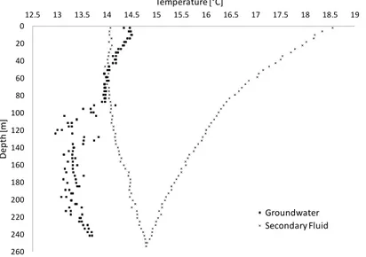
Figure 7. Ground temperature profile around BHE7 39

Figure 8. BHE7: U-pipe with spacers 39

Figure 9. Connection of BHE7 to the heat pump evaporator 39

Figure 10. Fluid mean temperatures in each section during the whole

first DTRT in BHE4 40

Figure 11. Instantaneous fluid temperatures during heat injection 41 Figure 12. Instantaneous fluid and groundwater temperatures during

thermal recovery 42

Figure 13. Local ground thermal conductivities in U-pipe, BHE4 43

Figure 14. Local borehole resistances in U-pipe, BHE4 43

Figure 15. Standard deviation of measurements during undisturbed ground conditions (30 seconds integration and repetition time during

two hours) 45

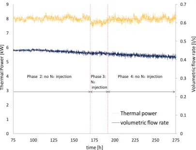
Figure 16. Thermal power and volumetric flow rate during the N2

injection DTRT 46

Figure 17. Average fluid temperature in each section during the N2

(16)

Figure 18. Fluid temperatures before and during N2 injection 47 Figure 19. Fluid and groundwater temperatures previous to N2 injection 48 Figure 20. Fluid and groundwater temperatures one hour after starting

N2 injection 48

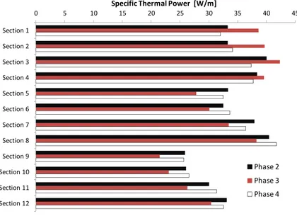
Figure 21. Average power distribution in the BHE during the different

DTRT phases 49

Figure 22. Average fluid to groundwater resistance along BHE4 with and

without N2 injection 50

Figure 23. Comparison of local thermal resistances obtained in BHE4 50 Figure 24. Temperature difference and heat injection in section 2 51 Figure 25. Temperature difference and heat injection in section 4 51 Figure 26. Temperature difference and heat injection in section 5 52 Figure 27. Instantaneous secondary fluid temperatures during the first

two hours of heat injection in BHE4 53

Figure 28. Flow rate and thermal power during heat injection

experiments in BHE7 53

Figure 29. Fluid and groundwater temperatures during heat injection in

BHE7 at four volumetric flow rates 54

Figure 30. Themal power distribution along the BHE7 up-going and

down-going shanks at different flow rates 55

Figure 31. Local average specific injected power 56

Figure 32. Fluid to groundwater ΔT 56

Figure 33. Fluid to groundwater resistance 56

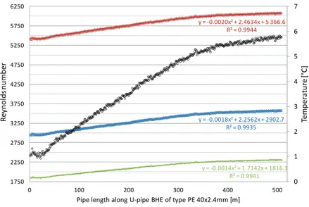
Figure 34. Fluid to groundwater thermal resistance vs. flow rate 57 Figure 35. Reynolds number at four different flows in U-pipe BHE 58 Figure 36. Heat transfer coefficient at four different flows in a U-pipe BHE 58

(17)

Figure 37. Fluid to inner pipe wall thermal resistances along the depth at

different flows 59

Figure 38. Reynolds number along the pipe length of BHE4 allowing the viscosity to change for given secondary fluid temperatures (flow 0.3 l/s) 60 Figure 39. Comparison of pressure drop in U-pipe with and without fiber optic cable having the same secondary fluid (see section 3.2.1) 60 Figure 40. Temperatures in BHE7 at short intervals after heat pump start

(at 0.4 l/s). 61

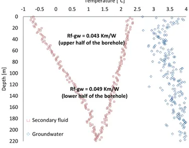
Figure 41. Secondary fluid and groundwater temperature profile at 0.36 l/s after elapsed residence time, including local fluid to groundwater

thermal resistance 63

Figure 42. Secondary fluid and groundwater temperatures at 0.81 l/s after elapsed residence time, including local fluid to groundwater thermal resistance 63 Figure 43. Secondary fluid and groundwater temperature at 0.60 l/s, after elapsed residence time, including local fluid to groundwater thermal resistance 64 Figure 44. Secondary fluid and groundwater temperatures at 1.00 l/s, after elapsed residence time, including local fluid to groundwater thermal resistance 64 Figure 45. Comparison of secondary fluid temperature profiles after elapsed residence time during the first heat extraction experiment in

U-pipe (ΔT≈3.5 K) 65

Figure 46. Comparison of secondary fluid temperature profiles after elapsed residence time during the second heat extraction experiment in

U-pipe (ΔT≈2.5 K) 66

Figure 47. Installation and illustration of the U-pipe thermosyphon 70 Figure 48. Temperatures along the riser during heat pump operation.

The heat pump starts at 15:40 and stops at 16:45 71

Figure 49.Temperatures along the riser during borehole recovery 71 Figure 50. Temperatures of the riser outer pipe wall at different depths in

(18)

Figure 51. Riser pipe wall and groundwater temperature at 16.02 73 Figure 52. Energy flows at the different components of the heat pump system during the heat pump cycle between 15:40 and 16:45 on April 6th 2009 74

Figure 53. Heat transfer coefficient along the depth in BHE12 75

Figure 54. Pipe to groundwater thermal resistance along BHE12 75

Figure 55. P-h diagram showing how the CO2 travels in BHE12 at four

simulated cases 76

Figure 56. Comparison between calculated CO2 temperatures along the

riser and measured temperatures in BHE12 76

Figure 57. Average calibrated temperatures and standard deviation along the fiber cable during a 25 hours measurement period (6 measurements

per hour). 77

Figure 58. BHE9: Pipe-in-pipe with PE40x2.4 central pipe 80

Figure 59. Cross section of BHE9 80

Figure 60. Sketch of the fiber optic loop in BHE9 80

Figure 61. Undisturbed temperature measurement along all fibers in BHE9 81

Figure 63. BHE10: Pipe-in-pipe with insulated central pipe 82

Figure 64. Sketch of the heat pump system connected to BHE10 82

Figure 65. Double-ended fiber calibration in BHE10. Undisturbed

ground conditions 83

Figure 66. Section division of BHE9 and BHE10 84

Figure 67. Evolution of temperatures during the DTRTs in BHE9 85

Figure 68. Evolution of temperatures during the DTRTs in BHE10 86 Figure 69. Comparison of fluid temperature profiles in BHE9 and BHE10 88

(19)

Figure 70. Thermal power distribution in BHE9 during DTRT1 89

Figure 71. Thermal power distribution in BHE9 during DTRT2 90

Figure 72. Thermal power distribution in BHE10 90

Figure 73. Reynolds number along the depth at two different flows in

Pipe-in-pipe BHE 91

Figure 74. Convection heat transfer coefficient at two different flows in

Pipe-in-pipe BHE 92

Figure 75. Thermal resistances in different central pipe polyethylene (λPE=0.42 W/mK) alternatives. Convection resistances calculated at 0.5

l/s using ν= 1.14x10-6_m2_{/s, λ=0.58 W/mK, and Pr=10.4.} ₉₃

Figure 76. Pressure drop in Pipe-in-pipe BHE 94

Figure 77. Comparison of convection thermal resistances in a pipe-in-pipe BHE at different Reynolds numbers in the annulus. Calculated using ν=1.14x10-6_m2_{/s, λ=0.58 W/mK and Pr=10.4. Central pipe of}

type PE40x2.4mm. 95

Figure 78. Residence time through BHE10 at different volumetric flow rates 96 Figure 79. Inlet, outlet, and average borehole wall temperatures at 0.6 l/s 97 Figure 80. Development of the fluid profile in BHE10 at 0.6 l/s 98 Figure 81. Instantaneous fluid and borehole wall temperature profiles during heat pump operation at different volumetric flow rates in BHE10 98 Figure 82. Annulus to borehole wall thermal resistance during heat pump

operation at three flow rates 99

Figure 83. Inlet and outlet temperatures during days with ambient

temperatures between 0 and 12 °C (December 2011) 100

temperatures between -2 and 12°C (January 2012) 100

(20)

temperatures between -18 and 0°C (February 2012) 101

Figure 87. BHE3: Installation of the Multi-chamber BHE installation 104 Figure 88. Measured volumetric flow rate with two different meters

during TRT1 and TRT2 in BHE3 106

Figure 89. Temperatures during TRT1 in BHE3 (secondary fluid going

down through the central pipe) 107

Figure 90. Temperatures during TRT2 in BHE3 (secondary fluid coming

up through the central pipe) 107

Figure 91. Comparison of pressure drop in U-pipe and Multi-chamber BHE 108 Figure 92. Net thermal power distribution in Multi-chamber BHE

(BHE3) during TRT1 110

Figure 93. Net thermal power distribution in Multi-chamber BHE

(BHE3) during TRT2 110

Figure 94. Comparison of two fluid mean temperature approaches

during TRT1 in BHE3 111

Figure 95. Comparison of two fluid mean temperature approaches

during TRT2 in BHE3 112

Figure 96. Measurements in BHE3 at 0.80 l/s during heat pump

operation. Downward flow in central pipe. 113

Figure 97. Measurements in BHE3 at 0.80 l/s during heat pump

operation. Upward flow in central pipe. 113

Figure 98. Comparison of the net thermal power absorbed as the fluid travels downwards in two different flow directions at a rate of 0.80 l/s 114 Figure 99. Comparison of the net power absorbed as the fluid travels upwards in two different flow directions at a rate of 0.80 l/s 114

(21)

Figure 102. Installation of BHE11 117

Figure 103. Connection points to BHE11 118

Figure 104. Undisturbed temperature profile in BHE11 118

Figure 105. Section division of BHE11 during DTRT analysis 119

Figure 106. Temperature and thermal power evolution during all DTRTs

in BHE11 119

Figure 107. Heat flow from section 1 120

Figure 108. Heat flow from section 4 121

Figure 109. Fluid temperature profiles at two different volumetric flow rates. Secondary fluid travels downwards through the external pipes 121 Figure 110. Local borehole resistance results obtained after analyzing all DTRTs 123-124 Figure 111. Heat transfer coefficient along the measured peripheral pipe

in each section 125

Figure 112. Heat transfer coefficient at two different flows along BHE11 126 Figure 113. Reynolds number distribution at two different flows along BHE11 126 Figure 114. Secondary fluid temperatures at the inlet, bottom and outlet points of the multi-pipe BHE during a day of measurements at 0.13 l/s 128 Figure 115. Temperature profiles during heat pump start up at 0.20 l/s 128 Figure 116. Comparison of measured temperature profiles in BHE11 at different flow rates during heat pump operation (residence time has not

(22)

I n d e x o f t a b l e s

Table 3-1. Chronology of the bubble injection DTRT 44

Table 3-2. Standard deviation of the measured flow rates during heat

injection in BHE7 54

Table 3-3. Characteristics of the heat extraction experiment with ΔT≈3.5 K 63 Table 3-4. Characteristics of the heat extraction experiment with ΔT=2.5 K 64 Table 3-5. Heat extraction percentage along each half of the BHE7 tubes

during the first heat extraction experiment (ΔT≈3.5 K) 66

Table 3-6. Heat extraction percentage along each half of the BHE7 tubes

during the second heat extraction experiment (ΔT≈2.5 K) 66

Table 5-1. Global thermal resistance results from BHE9 and BHE10 87 Table 6-1. Effective ground and borehole resistance during TRT1 and TRT2 108 Table 6-2. Standard deviation of temperature measurements during

TRTs in BHE3 109

Table 7-1. Chronology of the different parts of the heat injection test in BHE11 119

(23)

1 Introduction

1 . 1 G e n e r a l o b j e c t i v e

The aim of this thesis is to suggest methods for reducing the temperature difference between the ground and the secondary fluid in borehole heat exchangers.

1 . 2 C o n t e x t o f t h e r e s e a r c h

A Borehole Heat Exchanger (BHE) consists of one or several bore-hole(s) drilled into the ground allowing heat to be exchanged between the ground and a fluid circulating in the borehole(s).

Depending on whether there are one or several boreholes, the word “Single” or “Multiple” can be added, resulting in a simple classification subject to the amount of boreholes, “Single BHEs” or “Multiple BHEs”. The fluid circulation normally takes place in an embedded collector pipe inside the borehole, but there are also open systems where the fluid is in direct contact with the surrounding soil or rock. BHEs are often con-nected to another heat exchanger at the ground surface level, commonly (but not always) the evaporator of a Ground Source Heat Pump (GSHP).

The most common single BHE is the U-pipe, where the secondary fluid travels down- and upwards through two equal tubes joined together at the bottom. There is also the coaxial type, classified depending on the geometry as pipe-in-pipe, multi-pipe, or multi-chamber (Figure 1). Pipe-in-pipe BHEs consist of a central pipe inserted into a larger tube (external pipe), forming an annular flow channel between them, as shown in Figure 1(a). A Multi-pipe design, Figure 1(b), consists of a cen-tral pipe connected at the borehole bottom with several smaller external and independent flow channels. The multi-chamber BHE is similar to the multi-pipe case, except that the central pipe and the external channels (so called chambers) are all part of a common pipe structure, as shown in Figure 1(c).

(24)

(a) (b) _(c)

Figure 1. Illustration of the different types of coaxial BHE geometries

GSHPs are a well established technology for heating and cooling build-ings. In 2010, over 100 000 GSHP units were sold in Europe, reaching a total of over one million installations (RHC, 2012). Worldwide, ap-proximately 2.94 million ground source heat pump systems covered 49.0% of the world’s used geothermal energy in 2010, accounting for 69.7% of the worldwide installed geothermal capacity (Lund et al, 2010). In Sweden, up to 12 TWh of cooling and heating are delivered yearly by this type of system (GEOTEC, 2012). About 30 000 units were sold dur-ing 2011 around the country, a number that has been relatively stable during the last years (SVEP, 2012). The low running costs have encour-aged users to install GSHPs in spite of their relatively high installation cost. Statistics also show that the efficiency of these systems has substan-tially improved along the years.

Although the technology is well known, there still remain several techni-cal aspects to be improved on which research should be addressed. Im-proving borehole heat exchangers was recently pointed out by (Spitler and Bernier, 2011) and by the European Platform for Renewable Heat-ing and CoolHeat-ing (RHC, 2012) as one of the focal research areas for the near future. It is known that a reduction of 1 K in the temperature dif-ference between the ground and the evaporator of a GSHP can increase the heat pump Coefficient of Performance (COP) by 2 to 3%.

In order to find methods for increasing the COP by 6-9% and to in-crease the level of understanding of BHEs, this thesis mainly addresses the local thermal processes in several types of single BHEs.

Instead of conventional thermal response tests based on inlet and outlet fluid temperature measurements (limited to giving merely average and global information about the BHE performance), a new technique called Distributed Thermal Response Test (DTRT) is the main method used here, giving detailed information about the tested BHEs thanks to the application of Distributed Temperature Sensing (DTS).

Borehole wall Central pipe External pipe Borehole wall Central pipe External pipes

(25)

1 . 3 D i s t r i b u t e d t e m p e r a t u r e

s e n s i n g i n B H E s

DTS is based on Raman optical time domain reflectometry, consisting of the injection of laser light pulses through a length of optical fiber and the subsequent detection of a non-linear part of the reflected light that is re-emitted with a different frequency than the input signal, a backscat-tered signal that travels through the whole fiber. This frequency shifted light scattering is called Raman scattering, and the temperature is deter-mined by analyzing it over a period of time (integration time) for a given cable section.

The re-emitted Raman scattered light has one part at lower frequencies (stokes) and another at higher frequencies (anti-stokes) than the original injected light. The low and high frequencies are related to the energy gap between them. The ratio between their intensities depends only on tem-perature, meaning that the temperature can be determined at a certain section as a function of the ratio between stokes and anti-stokes backscattered light.

The differential loss between anti-stokes and stokes that affects the tem-perature reading in proportion to the distance from the measurement in-strument is adjusted. The loss is normally within the order of 0.3 decibels per kilometer with lasers operating at around 1064 nm (wavelength in fi-ber systems vary from 850 to 1300 nm). This loss, often called attenua-tion, limits the signal traveling distance and can also be induced by hu-man installation errors.

The precision of a DTS measurement depends on the fiber index of re-fraction (ratio comparing the speed of light in a vacuum to the speed of light in a medium, normally of around 1.35 in fibers), the amount of in-formation read by the data acquisition instrument per unit time, and on the size of the observed section along the fiber. Better accuracy is ob-tained when more photons are observed per unit time. However, the photon density decreases with increasing length of the measurement sec-tion, meaning that the amount of information read by the instrument in a certain period of time may also be smaller if the distance to the ob-served section is large.

With known travel time and velocity, it is possible to identify the source of the Raman scatter, i.e. the position where a signal comes from. This is carefully done accounting for the delay between the instant of light injec-tion to observainjec-tion of the backscatter arrival, subsequently trimming the signal in order to account for light dispersion within the fiber.

(26)

DTS instruments integrate the signals and determine an average temper-ature for different continuous sections. The length of these sections de-pends on the instrument specifications and the most powerful instru-ment in the market today has a sampling resolution of 12.5 cm. A section of the fiber located far away from the instrument needs a longer integra-tion time because the amount of informaintegra-tion coming back to the in-strument decreases with the distance (the light signal becomes exponen-tially weaker as it travels through the fiber).

Different integration instruments have different so called spatial resolu-tions, the least width of a temperature change that it can detect. The best spatial resolution today goes down to 0.25 cm. A step temperature change having a width lower than the instruments spatial resolution re-sults on a measured temperature affected by a factor approximately pro-portional to the ratio between the spot width and the spatial resolution. The expected precisions for temperature, time, and space, must be com-promised in order to achieve the desired measurement quality. Longer measurement time give better temperature resolution, larger spatial aver-aging gives better temperature resolution, and temperature resolution de-creases with distance due to attenuation.

The intensity of the laser varies between different DTS instruments and the fiber characteristics change from manufacturer to manufacturer. In order to guarantee quality on distributed temperature measurements, a careful calibration process must be carried out. This normally requires the adjustment of an offset (Raman conversion coefficient correction) and a slope (differential loss correction).

Typically, the whole measuring process is carried out in single ended mode, the laser pulses are sent in one direction along the fiber. If a fiber is looped having two connectors to the instrument (one at each fiber end), a combined measurement commonly known as double-ended measurement can be made. In the latter case, sending the pulses from each end allows for signal compensation based on two measurements, giving simultaneous correction of differential losses and attenuations. The offset correction may still be necessary.

The measurements in this thesis have been done in single and double ended mode, depending on the installation. All installations use multi-mode fiber cables having an external diameter of 3.8 mm. Although the readings are given in terms of BHE/fiber lengths, the borehole devia-tions have been disregarded and the word “depth” has, for didactic rea-sons, been used along this thesis when referring to the length.

(27)

The calibration process in all experimental installations has consisted of placing two or more relatively long fiber sections into one or even two environments with a known temperature such as an ice bath. These ref-erence sections are separated from each other by twice the borehole depth and are, at least, located before and after the fiber inside the bore-hole. The integration instrument has also been kept at constant room temperatures during calibration and measurements.

Besides the trade off made at each installation site regarding the spatial, time and temperature accuracy of the instrument, a systematic uncertain-ty when measuring inside BHEs might arise due to the unknown posi-tion of the fiber optic cable in the borehole/pipes, specially at laminar flow conditions. For turbulent flow, for instance, it is well known that the temperature profile is flat across the pipe outside the thermal bound-ary layer at the pipe wall.

This possible systematic uncertainty has been handled by estimating the laminar sub-layer at the pipe wall within which heat is transferred only by thermal conduction. The temperature difference between the pipe wall and the inner border of the boundary layer is calculated for each case. With known pipe dimensions, fluid thermo-physical properties, fluid ve-locity, and heat flux from or to the ground, it is possible to estimate the convection heat transfer coefficient and thereby the temperature differ-ence between the pipe wall and the bulk fluid temperature, resulting in an indication of where across the pipe the temperature change takes place during laminar or turbulent flow.

On the groundwater side, the risk to fall into this type of systematic error depends on the radial temperature gradient between the collector pipes and the borehole wall, which depends on the heat extraction/injection rate, volumetric flow rate, type of heat exchanger, and the temperature levels. This is discussed in connection to specific tests where measure-ments on the groundwater side are evaluated.

For more details about generalities of the DTS technique and their use in BHEs, the reader is referred to (Selker et al, 2006), (Tyler et al, 2009), and (Acuña, 2010), among others.

(28)

2 Previous work

As this thesis is a experimental study on the thermal response of U-pipe and coaxial heat exchangers in groundwater filled boreholes, this chapter is dedicated to giving a theoretical background about the four different active parts that can be distinguished inside a heat exchanger installed in a ground-water filled borehole. These are the ground, the collector pipes, the groundwater filling the space between the borehole wall and the pipes, and a fluid circulating inside the collector pipes (the secondary flu-id). Previous work concerning the study of the thermal processes in the-se borehole heat exchanger parts is surveyed in the-sections 2.1 through 2.4.

2 . 1 T h e g r o u n d t h e r m a l r e s p o n s e

The thermal process in the ground has mainly been studied as a time de-pendent three dimensional heat conduction problem, rarely accounting for the effects of groundwater movement. The heat transfer from the borehole wall to the ground depends on the ground thermal conductivi-ty, the thermal diffusiviconductivi-ty, and the undisturbed ground temperature. The different heat transfer forms with origin in the heat conduction equation are mainly linear partial differential equations, and their solu-tions can be superposed, as mathematically proven in (Claesson et al, 1985). The transient thermal response to thermal loads from the BHE is superposed on the natural stationary temperature distribution that previ-ously existed in the ground. Analytical one-dimensional heat conduction models treating the heat transfer outside the borehole such as the Infi-nite Line (Ingersoll and Plass, 1948) and Cylinder Source (Carslaw and Jaeger, 1959) have been used for many years to study these problems, as well as the finite difference two dimensional g-function introduced by (Eskilson, 1987).

The Infinite Line Source (ILS) model assumes the thermal load to be a line source of constant heat rate and infinite length surrounded by an in-finite homogeneous ground. The cylinder heat source model assumes the borehole as a cylinder surrounded by homogeneous ground and having constant heat flux across its periphery; and the g-function (mostly used for multiple BHE problems) gives a relation between the heat exchange with the ground and the temperature at the borehole wall. Another

(29)

ap-proach is the Finite Line Source Solution (FLS) which considers the fi-nite length of the boreholes, also presented in (Eskilson, 1987) but fur-ther developed by (Zeng et al, 2002) and (Lamarche and Beauchamp, 2007).

None of the above mentioned models really consider the thermal capaci-ty effects inside the borehole and, for a single borehole, their solutions (ILS, cylinder source, FLS, and g-function) meet after a few hours and are the same as long as the heat transfer is essentially one dimensional in the radial direction. The cylinder line source and the g-function are equal from the beginning. The same happens with ILS and FLS solutions. This is because the former two account for heat being exchanged at the bore-hole wall while the line source solutions assume that heat is exchanged from/to the center of the borehole.

The ILS model, which has been used at a local level throughout this the-sis, evaluates the temperature response at radius r after time t of a step change in supplied heat, allowing that the temperature response of many heat steps at different times may need to be superposed. A thermal re-sistance R can be also added to the ILS model in order to represent the temperature difference between the secondary fluid and the borehole wall as suggested by (Mogensen, 1983).

The infinite line source approach is, for instance, commonly used for measuring the ground thermal conductivity and the thermal resistance R through Thermal Response Tests (TRT), where the ground thermal re-sponse to a few days of constant heat injection or heat extraction is ana-lyzed in order to obtain this information. The cylindrical source model as well as numerical evaluation methods have also been used, even to calcu-late the thermal conductivity along the depth (Fujii et al, 2006). Many times the evaluation accounts for the above described superposition of the response to heat steps and/or use parameter estimation techniques such as suggested in (Shonder and Beck, 1999). The FLS method has al-so been used for TRT analyses by (Bandos et al, 2011).

The TRT method was first used by (Mogensen, 1983) and then by (Eskilson et al, 1987) and (Claesson and Hellström, 1988), and it is now extensively used worldwide in the academy and commercially after the work presented by (Gehlin, 2002), at Luleå University of Technology at the same time as it was developed at Oklahoma State University. IEA Annex 21 (http://www.thermalresponsetest.org/), at the moment on fi-nal reporting stage, has studied and collected a large amount of infor-mation about TRTs. The reliability of this method as compared to labor-atory core tests was recently demonstrated by (Liebel, 2012).

(30)

The borehole thermal resistance R has traditionally been denoted Rb after (Claesson and Hellström, 1988) and (Hellström, 1991), representing today a well established parameter for characterizing BHEs. It is a ther-mal resistance per unit length of the borehole [K/(W/m)], and it is typi-cally used assuming that the fluid temperatures of the downward and upward flow are the same. Experimentally, Rb is normally found during steady-flux conditions achieved with TRT tests, in order to avoid ac-counting for thermal capacitance effects in the borehole.

As the fluid temperatures obtained from a single BHE are influence by the surrounding ground but also by Rb, an example shown in Figure 2 presents the effect of the borehole resistance Rb on the secondary fluid mean temperature exiting from the BHE calculated using ILS. It is seen that the same fluid temperature can be obtained with different heat ex-traction rates by changing the BHE. The temperature difference between the highest and lowest fluid temperature becomes larger with increasing values of borehole resistance and heat rate in Watts per meter. A low Rb gives a low temperature difference between the fluid and the ground.

Figure 2. Mean fluid temperature variation with borehole resistance and specific heat extraction rates (calculated for one day of constant operation with λrock=2.5 W/mK,

α=1.25x10-6_m2_{/s, and T} rock=8°C)

In commercial software such as those by (Hellström and Sanner, 1997), (Spitler, 2000), and (Kavanaugh and Rafferty, 1997), the calculation of the borehole resistance is done for steady-state conditions. Commercial software concentrate mostly on what happens in the surrounding ground and are mainly devoted to calculating the long term borehole wall

tem-‐4 ‐2 0 2 4 6 0 0.01 0.02 0.03 0.04 0.05 0.06 0.07 0.08 0.09 0.1 Tf [° C ] Rb[Km/W] 10 W/m 20 W/m 30 W/m 40 W/m 50 W/m

(31)

peratures for multiple BHEs using spatial and temporal superposition. The theory behind the solutions is the above mentioned Eskilson’s g-functions, which are based on the so called Superposition Borehole Model (SBM), explained in detail in (Eskilson, 1986).

For multiple BHEs, g-functions can also be generated with the FLS model, and the simulated solutions for variable heat load can also be su-perposed in time to describe the ground response of any BHE geometry. FLS generated g-functions are based on a constant heat flux at the bore-hole periphery as boundary condition and they seem to fit to some ex-tent with the g-functions generated with SBM, besides a certain degree of overestimation (Fossa, 2011). Numerical solutions are more time con-suming while analytical FLS calculations allow the rapid and flexible study of the thermal response of any field geometry. (Fossa et al, 2009) is an example on the use of the FLS approach.

The g-function concept has, sometimes with limitations (including U-pipe geometry normally modeled with a single cylinder having equivalent diameter, negative borehole wall temperatures for very short times, lack of thermal interaction between pipes, neglecting thermal capacity of the secondary working fluid, among others), been extended to shorter time steps by modeling the heat transfer from the fluid to the borehole wall through the inclusion of the thermal resistances and even capacitances inside the borehole. This has partially been studied in (Yavuzturk and Spitler, 1999), (Yavuzturk and Spitler, 2001), (Yavuzturk et al, 2009), (Beier and Smith, 2003), (Bandyopadhyay et al, 2008), (Lamarche and Beauchamp, 2007), (Javed and Claesson, 2011) and (Claesson and Javed, 2011). Including shorter time steps is important in order to better ac-count for peak loads where the secondary fluid, the pipe, and the filling material inside the borehole, can perhaps dampen the temperature re-sponse of the ground. A large heat capacity is normally desirable in BHEs in order to avoid rapid temperature changes during short heat pump operation periods. More about what happens inside the borehole is documented in section 2.3.

Although water movement in the ground has not been studied as much as the heat conduction problem, it is important to be aware that it may influence the thermal processes in a BHE. Some studies about the influ-ence of groundwater flow in the design of multiple BHEs are those by (Claesson and Hellström, 2000), (Chiasson et al, 2000), and (Bauer et al, 2012).

(32)

2 . 2 G r o u n d w a t e r - f i l l e d b o r e h o l e s

Groundwater filled boreholes are common in North European coun-tries. It has been shown that natural convection is induced by the tem-perature gradients around the BHE. Conductive heat transfer has been found to still be dominant, i.e. calculated borehole thermal resistances were only 1.2 to 1.3 times higher than experimental (Claesson and Hellström, 1988). The magnitude of the natural convection depends on the heat transfer rate and the temperature level (Kjellsson and Hellström, 1997).

(Witte and Van Gelder, 2006) studied the effect of natural convection by imposing so-called multi-level heating and cooling pulses. Similar ap-proaches were later used by (Gustafsson and Gehlin, 2006), (Gustafsson and Gehlin, 2008), (Gustafsson et al, 2010), and (Gustafsson and Westerlund, 2010), who evidenced the presence of natural convection through multi-level-injection TRTs. The works from Gustafsson et al. found that heat transfer in the groundwater inside the borehole was about three times better with temperature induced natural groundwater movement as compared to stagnant water at temperature levels between 10 and 35˚C. A suggestion to using different equivalent diameter approx-imations depending on the TRT circumstances was pointed out.

(Kharseh, 2011) and (Liebel, 2012) imposed forced convection condi-tions in the groundwater by N2 injection at the borehole bottom and us-ing a submersible pump, respectively. They found larger effects on the effective borehole resistance than those found in natural convection, as expected.

The alternative to groundwater-filled boreholes is a backfill material, or grout, commonly used in USA, central and southern Europe. These are used to prevent contaminants from migrating along the axis of the bore-hole. In some countries, grouting materials are used by law even when no risks for contaminant migration exist. Cement and bentonite based materials with additives are mainly used. It is normally preferred to use highly conductive grouting materials for enhancing the heat transfer from the borehole wall to the collector pipes.

A disadvantage of highly conductive grout is that it also increases the thermal shunt flow between the down-going and up-coming secondary fluid flows. Grouted BHEs may also be thermally unstable for a long time after installation, as shown by (Montero et al, 2012). Proposals are at the moment being studied for guaranteeing the proper use of these materials (Anbergen et al, 2012). Even groundwater movement in grout-ed BHEs can occur (Fujimoto et al, 2012). No expressions for calculat-ing heat transfer specifically in the groundwater of groundwater-filled

(33)

boreholes have been presented, in contrast to the grouted case, which has been studied by several researchers (Paul, 1996), (Hellström, 1991), (Sharqawy et al, 2009).

If the thermal conductivity of the grout is lower than in the surrounding ground, a smaller diameter borehole may reduce the borehole resistance. With a large borehole diameter the collector pipes could be placed close to the borehole wall and apart from each other, making a better BHE, thereby reducing the thermal resistance Rb. Also, if the thermal capaci-tance of the grout is high, the short term performance of the heat ex-changer may be improved. Results from five thermal response tests in U-pipe BHEs, where different grouting material were used, illustrate these effects (Bose et al, 2002). (Hellström, 1998) presented calculated thermal resistances using different borehole filling materials with three different U-pipe positions in the borehole.

A literature survey covering practical aspects of grouted boreholes from a Swedish perspective was recent presented by (Hjulström, 2012).

2 . 3 T h e c o l l e c t o r p i p e s

The collector pipes are typically made of medium density polyethylene, a flexible material having a thermal conductivity of 0.42 W/mK, which is high for a plastic, and offering good mechanical properties for this appli-cation. There are also some few exceptions with pipes made of stainless steel, copper, PVC and other types of plastic.

Two general BHE types are known depending on the geometry: U-pipe (single, double, or triple; including the use of spacers for separating the shanks) and coaxial BHEs. The amount of pipes and their geometrical arrangement allows classifying them in several other categories accord-ingly as presented in section 1.2.

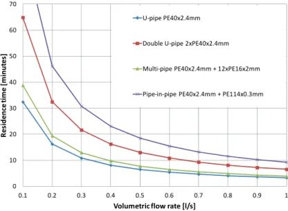
Each BHE type may demand specific flow rates for operation at opti-mum conditions, i.e. low borehole resistance, low thermal shunt flow be-tween pipes, long enough fluid residence time, among others. Different fluid residence times are, as an example, shown in Figure 3, illustrating how long time a fluid plug takes to travel through the whole heat ex-changer at different flow rates. Regarding the thermal resistances in BHEs, a literature survey covering all types of BHEs is presented in sec-tions 2.3.1 and 2.3.2.

(34)

Figure 3. Residence time of BHE types tested in this thesis (100 m deep borehole)

2 . 3 . 1 U - p i p e B H E s

U-pipe BHEs represent the most common method to exchange heat with the ground today, having standard dimensions of 40 mm outer di-ameter and 2.4 mm wall thickness. Their thermal performance is poor due to thermal shunt flow between pipes and undesirable pipe placement relative to the borehole wall.

Theoretical studies on U-pipe BHEs have dominated the single BHE re-search work published until now. (Claesson and Bennet, 1987) and (Claesson and Hellström, 2011), for example, computed the heat flows between the pipes (located at any position) and the outer rock. (Hellström, 1991), (Zeng et al, 2003) and (Diao et al, 2004) are other ex-amples of extensive studies of U-pipe BHEs where mathematical expres-sions for calculating a borehole resistance for the case of uniform bore-hole wall temperature and uniform heat flux along the depth were devel-oped. Also, (Claesson and Eskilson, 1988) show calculated borehole thermal resistances for laminar and turbulent flow in three different U-pipe configurations, including cases surrounded by frozen water. It is clear that laminar flow in the pipes should be avoided as it increases the thermal resistance between the fluid and inner pipe wall. The calculations for the unfrozen cases were done considering only conduction heat transfer. 0 10 20 30 40 50 60 70 0.1 0.2 0.3 0.4 0.5 0.6 0.7 0.8 0.9 1 R e si de nc e ti m e [ m inut e s] Volumetric flow rate [l/s] U‐pipe PE40x2.4mm Double U‐pipe 2xPE40x2.4mm Multi‐pipe PE40x2.4mm + 12xPE16x2mm Pipe‐in‐pipe PE40x2.4mm + PE114x0.3mm

(35)

Calculating borehole thermal resistances has, in many studies, been done based on the use of the arithmetic fluid mean temperature. (Marcotte and Pasquier, 2008) argued that this may lead to an overestimation of the borehole resistance and introduced an approximation where the circulat-ing fluid temperature varies linearly along the flow path. (Lamarche et al, 2010) used 2D and 3D numerical simulations to evaluate different meth-ods. Other articles including study of thermal resistance in U-pipe BHEs are (Du and Chen, 2011) and (Beier, 2011), (Bauer et al, 2011). (Zarella et al, 2011) improved and validated the work by (De Carli et al, 2010), a ca-pacity resistance model that studies the behavior of BHEs in some bore-hole field configurations.

Almost all the above mentioned papers, except for (Eskilson et al, 1987), (Gehlin, 2002), (Bose et al, 2002), and (Witte and Van Gelder, 2006) use numerical and not measured results as a reference. Many times, just in and outlet temperatures are used for model validation. An experimental article providing data sets for U-pipe BHEs and for ground thermal conductivity estimates is (Beier et al, 2011), where a sand box with a large amount of temperature measurement points is used for laboratory controlled experiments.

2 . 3 . 2 C o a x i a l B H E s

The first multi-pipe BHE ideas were introduced by Ove Platell in Swe-den, who wrote several publications (in Swedish) about this heat ex-changer. (Platell, 2006) discussed the thermal advantages of this design that operates with laminar flow in the peripheral pipes. Tests of a first prototype achieved thermal resistances between 0.009 - 0.028 Km/W (Hellström and Kjellsson, 2000). It consisted of 62 thin peripheral pipes (diameter of 3.8 mm and thickness of 0.65 mm) arranged close to the borehole wall in a special laboratory installation. The diameter of the la-boratory “borehole” was 104 mm.

(Oliver and Braud, 1981) presented an analytical solution of annular heat exchangers under steady state operation (using a constant temperature boundary condition 1 m away from the borehole wall), having limited practical application due to the purely transient process around the bore-hole in reality. Later, (Mei and Fischer, 1983) presented a study of a 50 m deep borehole with a polyvinylchloride (PVC) pipe-in-pipe BHE. The borehole had a diameter of 200 mm, and was backfilled with sand. Spac-ers were used in order to center the central pipe and temperature sensors were installed along the depth approximately every 7.5 meters inside and outside the annular channel as well as at the inlet and outlet. Although this borehole instrumentation was good, the measurements taken had certain limitation for validating the BHE model due to the high thermal resistance in the external PVC pipe, resulting in differences of up to 0.9

(36)

K from the measurements during continuous operation. During cyclic operation, predicted fluid temperatures at 16.8 m depth in the annulus matched very well with the measurements. Outside the outer PVC pipe, an asymptotic behavior of the temperatures showed that it almost does not feel the cyclic temperature behavior inside. On the other hand, it just decreases or increases slowly (during heat extraction or injection, respec-tively). Besides this experimental work, an analytical model presented in (Mei and Fischer, 1983) is compared to the measurements and allows discussing the effects of geometry variations, flow rate, among others, including the ground thermal response.

(Hellström, 1994) and (Hellström, 2002) described experiments where the secondary fluid travels in direct contact with the rock, with only a single central pipe. Turbulent operating conditions resulted in Rb of circa 0.01 Km/W, while drastically higher resistance values were found for laminar flow, Rb 0.12 Km/W, (the latter also due to the central pipe ec-centricity). The same year, (Yavuzturk and Chiasson, 2002) showed that pipe-in-pipe BHEs have potential for a very low Rb.

Older work regarding coaxial BHEs from the early 1980s is presented in the EU project GROUNDHIT where a pipe-in-pipe prototype was sug-gested (Sanner et al, 2007). (EWS, 2006) also describes the GROUNDHIT design, which consisted of one PE 63x5.3 mm outer pipe with an inner channel with dimensions PE 40x3.7mm. Installation and assembling methods were tested and presented. However, the ther-mal resistances of this BHE were high due to material therther-mal proper-ties, thermal shunt flow, and distance to borehole wall.

The effects of flow rate and of thermal short-circuiting (and methods to avoid it) are studied based on a numerical model in (Zanchini et al, 2010) but no experiments are done. These effects are studied further in (Zanchini, et al, 2010b), where an outer pipe made of stainless steel is driven into the ground without having any grouting. (Witte H. , 2012) presented the development of another coaxial BHE called GEOTHEX, consisting of a pipe-in-pipe design having an insulated central pipe with helical vanes on its outer part. This BHE still had a high borehole ther-mal resistance, but a rather good installation method. A similar pipe-in-pipe geometry consisting of a steel helix placed in the annular zone was studied in (Zarella et al, 2011). The helix is welded around a central steel pipe which contains an insulated polyethylene tube inside. The fluid cir-culated in direct contact with the ground. The BHE was studied extend-ing the approach of (De Carli et al, 2010) and carryextend-ing out simple tem-perature measurements. This coaxial BHE had a good performance.

(37)

2 . 3 . 3 T h e r m o s y p h o n B H E p i p e s

The secondary fluid circulating inside these U-pipe and coaxial BHEs is commonly pumped with an electrically driven pump. However, the cir-culation in thermosyphons is driven by fluid density differences.

(Sanner, 1991) pointed at the importance of using appropriate pipe mate-rials that tolerate the pressure levels at which thermosyphons operate and that are suitable from the corrosion point of view (e.g. for long-term contact with groundwater).

(Kruse and Russmann, 2005) studied a design consisting of a counter-current liquid-vapor BHE consisting of a corrugated stainless steel heat pipe, a dozen of which have been installed on a commercial basis in Germany and Austria (Kruse and Peters, 2008). The number of known commercial heat pump installations using natural circulation was about 100 between 2001 and 2005, according to (Rieberer et al, 2005), a study that shows results from two 65 m deep self circulating BHEs, having a heat extraction rate of 58 W/m. Here, the probe head was identified as the bottleneck of these systems (they must guarantee a small pressure drop and good heat transfer at operating conditions).

Most work carried out until today correspond to solutions implying counter-current flow between the liquid and gas phases of the fluid, with the exception of (Ochsner, 2008), who presented a design consisting of a 40 mm flexible high-grade steel corrugated heat pipe system with the same working principle, but used as single or two tubes. The proposed two tube arrangement is in fact a coaxial design, where the liquid phase falls down through a central pipe and the liquid/vapor phase flows up-wards through an annular channel, i.e. between the central pipe and the inner wall of the external pipe. Heat extraction rates of about 50 W/m are mentioned. The installation of this BHE is done with an unwinding device, similar to those used in common polyethylene pipe installations.

2 . 4 T h e s e c o n d a r y f l u i d

When connected to a ground source heat pump, the circulating fluid in BHEs is commonly called secondary fluid, given that the primary fluid (or refrigerant) is circulating inside the heat pump itself. Other names such as brines are also often used. However, brines originally refer to salt based solutions, which rarely is the case.

A secondary fluid normally varies from water to an antifreeze aqueous solution of ethanol, glycol, etc. or a salt. There are also natural circulation probes or thermosyphons using fluids as carbon dioxide, able to change phase at typical ground temperature levels.

(38)

2 . 4 . 1 A q u e o u s a n t i f r e e z e s o l u t i o n s

Aqueous solutions of different additives, used instead of water, reduce the freezing point of the secondary fluid. Depending on the additive and its concentration, the thermophysical properties such as density, specific heat, viscosity, Prandtl number, etc., change; meaning that the choice of fluid has an important influence on the hydrodynamic and thermal per-formance of the system. A comprehensive study of the thermophysical properties of different secondary fluids is found in (Melinder, 2007). Ethanol plus water is the most common secondary fluid used in Sweden. As an example, Figure 4 shows how the ethanol concentration affects the kinematic viscosity of the fluid at different operating temperatures.

Figure 4. Viscosity of ethanol concentrations at different operating temperatures

Many other secondary fluids including salt solutions, their thermophysi-cal properties, and their usage potential were largely studied in (Melinder, 2007) and the reader is referred to this document for details. An interest-ing report where potassium carbonate is compared to other secondary fluids is (Melinder et al, 1989).

2 . 4 . 2 F l u i d s f o r t h e r m o s y p h o n s

Since phase change takes place inside the collector pipes, the condition for the secondary fluid in thermosyphon BHEs is its capacity to evapo-rate and condense at the temperature levels of a specific location. Carbon dioxide and propane are two examples of fluids that have been studied and used in this context.

1.0E‐6 2.0E‐6 3.0E‐6 4.0E‐6 5.0E‐6 6.0E‐6 7.0E‐6 8.0E‐6 ‐4 ‐2 0 2 4 6 8 Kin em at ic vi sco si ty [m 2/s ] Operating temperature [°C] 24.4% by weight, Tfreezing = ‐15°C 15.9% by weight, Tfreezing = ‐8°C 8.0% by weight, Tfreezing = ‐3.4°C 0%, Tfreezing = 0°C

(39)

Since most of processes in thermosyphon BHEs occur in saturation state, the pressure levels in the fluid loops are determined by the bore-hole (or rock) temperature levels. Normal rock temperatures in countries with heating demand imply, for example, CO2 operating pressures of about 30-45 bar. The vapor density is high (approximately 7 times higher than the density of R-134a), resulting in a high volumetric refrigeration capacity (which leads to small volumetric flow rates and small pressure loss).

From the environmental point of view, CO2 has zero ozone depletion potential, a GWP equal to 1, it is non-explosive, non-flammable, moder-ately toxic, and non-reactive. In case of leakage, no environmental effects are caused in the groundwater and, on the building side, since CO2 is al-so odorless and colorless, the installation of CO2 gas detectors is rec-ommended in order to detect harmful gas concentrations.

The first investigations of CO2 BHEs were done by (Rieberer et al, 2002), whose first tests showed undesired CO2 superheat at the head of the borehole, a problem that was later solved. The temperature levels measured at different depths confirmed good operation of the system during the heat pump cycle. (Rieberer et al, 2004) presented details about mass flow rates, the refrigerant superheat temperature differences in the heat pump, different BHE probe heads (heat pump evaporator), and dis-cussed the number of probes to be inserted in a single borehole. Later, (Rieberer, 2005) added results from a computer model showing simulat-ed saturation temperatures in the probe heads at different filling concen-trations.

(Kruse and Russmann, 2005) studied the minimum charge to guarantee a liquid film along the whole length of the BHE that they tested. The fill-ing ratio was found to be directly related to the specific heat flux under which the thermosyphon worked. The requirement of higher filling rates to achieve higher heat fluxes became evident. Regarding visualization about what happens along the depth in pipes with natural circulation, (Kruse and Peters, 2008) presented measurements where temperatures varied between -1.5 °C and -3.0 °C along the pipe, while the inlet CO2 temperature to the heat pump was -3.9 °C.

(Grab et al, 2011) and (Storch et al, 2011) demonstrated and showed a heat pipe operating with propane and presented visual observations on the wetted areas and the transition from start to boiling conditions, re-spectively. (Storch et al, 2012) showed other results on selected solid sur-faces with similar systems.