Generalized multiobjective particle swarm optimization solver for spreadsheet models: application to water quality, A

A generalized multiobjective particle swarm optimization

solver for spreadsheet models: application to water quality

Water Resources Planning and Management Division, Dept. of Civil and Environmental Engineering, Colorado State University, Fort Collins

Darrell G. Fontane2

Water Resources Planning and Management Division, Dept. of Civil and Environmental Engineering, Colorado State University, Fort Collins

Abstract. This paper presents an application of an evolutionary optimization

algorithm for multiobjective analysis of selective withdrawal from a thermally

stratified reservoir. A multiobjective particle swarm optimization (MOPSO) algorithm is used to find nondominated (Pareto) solutions when minimizing deviations from outflow water quality targets of: (i) temperature; (ii) dissolved oxygen (DO); (iii) total dissolved solids (TDS); and (iv) potential of hydrogen (pH). The decision variables are the flows through each port in the selective withdrawal structure.

The MOPSO algorithm, implemented as an add-in for Excel, is able to find nondominated solutions for any combination of the four abovementioned objectives. An interactive graphical method was also developed to display nondominated solutions in such way that the best compromise solutions can be identified for

different relative importance given to each objective. The method allows the decision maker to explore the Pareto set and visualize not only the best compromise solution but also sets of solutions that provide similar compromises.

1. Introduction

Decision making in water resources planning and management frequently involves multiple objectives. As greater attention is being given to the

environmental and social aspects of water resources allocation and

management the need for effective multiobjective optimization approaches is increasing. Many of the developments in the area of multiobjective analysis in the United States have come from the field of water resources (Goicoechea et al. 1982).

In multiobjective optimization, a set of nondominated solutions is usually produced instead of a single recommended solution. According to the concept of nondominance, also referred to Pareto optimality, a solution to a

multiobjective problem is nondominated, or Pareto optimal, if no objective can be improved without worsening at least one other objective.

Traditional multiobjective optimization methods attempt to find the set of nondominated solutions using mathematical programming. In the case of nonlinear problems, the weighting method and the ε-constraint method are the

1

Dept. of Civil and Environmental Engineering, Colorado State University, 1600 W. Plum St. 26H, Fort Collins, CO 80521, Tel: 970/492-9899, abaltar@engr.colostate.edu

2

Dept. of Civil and Environmental Engineering, Colorado State University, B213 Engr. Building, Fort Collins, CO 80521, Tel: 970/491-5248, fontane@engr.colostate.edu

most commonly used techniques. Both methods transform the multiobjective problem into a single objective problem which can be solved using nonlinear optimization.

With the weighting method, nondominated solutions are obtained if all weights are positive, however not all Pareto optimal solutions can be found unless all objective functions as well as the feasible region are convex. Another disadvantage of this method is that many different sets of weights may produce the same solution, compromising the efficiency of the method. When the weights reflect the preferences of the Decision Maker (DM), the method gives the best-compromise solution, i.e. the solution which produces the highest utility to the DM. The ε-constraint method, on the other hand, does not require convexity but only leads to nondominated solutions if certain specific

conditions are satisfied (Miettinen 2001).

According to Coello Coello (2001), the first hints on the potential of evolutionary algorithms (EA) for multiobjective optimization occurred in the 1960s but this research area remained largely unexplored until mid 1980s. This author also highlighted two advantages of evolutionary algorithms that make them particularly suitable for multiobjective optimization, when compared to traditional mathematical programming techniques:

• EA work simultanously with a set of possible solutions, the so-called population, and several nondominated solutions may be found in a single run of the algorithm;

• EA are less sensitive to the shape or continuity of the Pareto surface. Since the mid 1980s, a growing number of evolutionary multiobjective optimization algorithms have been proposed in the literature (Fonseca and Fleming 1995). Some studies have attempted to compare different algorithms. Coello Coello et al. (2004) compared four different algorithms when applied to five different test problems. All test problems, however, involved only two objectives. Zitzler and Thiele (1999) compared another five methods with three test problems. Some of the methods compared were later improved.

Particle swarm optimization – PSO (Kennedy and Eberhart 1995) is one of the newest techniques within the family of evolutionary optimization

algorithms. The algorithm is based on an analogy with the choreography of flight of a flock of birds. Due to its fast convergence, PSO has been advocated to be especially suitable for multiobjective optimization (Coello Coello et al. 2004).

There are many variants of the single objective PSO but in most of them the movement of the particles towards the optimum is governed by equations similar to the following:

( )

( )

(

( )

( )

)

(

( )

( )

)

( )

( )

(

)

Where w is an inertia coefficient that has an important role balancing global (a large value of w) and local search (a small value of w), c1 and c2 are

constants (usually c1 = c2 = 2), r1 and r2 are uniform random numbers in [0,1], Pi is the best position vector of particle i so far, Pg is the best position vector of all particles so far, xi(t) is the current position vector of particle i, and vi(t) is

the current “velocity” of particle i. Mendes et al. (2004) suggests an inertia coefficient w of less than 1, while other authors recommend to start with larger values and decrease with time, for example from a value of 1.4 to 0.5 (e.g. Elbeltagi et al. 2005, Jung and Karney 2006). Coello Coello et al. (2004) highlighted the sensitivity of the standard PSO algorithm to the value of w and proposed the introduction of a mutation operator that assures an adequate global search while keeping a small value of w (suggested 0.4) which favors a refined local search.

Several applications with evolutionary multiobjective optimization have been recently reported in the water resources literature (e.g. Liong et al. 2001, Muleta and Nicklow 2005, Suen et al. 2005, Tang and Reed 2005, Kapelan et al. 2005). None of these applications, however, used multiobjective PSO. Jung and Karney (2006) compared the performance of single-objective Genetic Algorithm and PSO approaches to optimize the selection, sizing, and

placement of hydraulic devices for transient protection. The authors studied six different cases and concluded that both algorithms produced very similar results in most cases but the PSO found better solutions when the same population size and number of iterations were applied.

In this paper, a modified version of the multiobjective PSO (MOPSO) proposed by Coello Coello et al. (2004) is used with an application to analyze the problem of selective withdrawal from thermally stratified reservoirs. A graphical procedure to incorporate the DM’s preferences is also proposed, further exploring the set of nondominated solutions and displaying the best-compromise solution as well as families of solutions with similar

compromises.

2. Multiobjective Particle Swarm Optimization

In the MOPSO algorithm (Coello Coello et al. 2004), the performances of different particles are always compared in terms of their dominance relations. The main characteristic of this algorithm is the use of an external repository which stores nondominated solutions. The algorithm starts by generating an initial population. All the particles of this population are compared to each other and the nondominated particles are stored in the repository. The particles’ positions will be subsequently updated using the following:

( )

( )

(

( )

( )

)

(

( )

( )

)

i v P x R x

v +1 = ⋅ + 1⋅ 1⋅ − + 2⋅ 2⋅ − (3)

Where Rh is a solution selected from the external repository in each

iteration t, and the other terms have already been defined, with w = 0.4. The best position vector of particle i, Pi, is initially set equal to the initial

position of particle i. In the subsequent iterations, the best position vector is updated in the following way: (i) if the current Pi(t) dominates the new

Pi(t) then Pi(t+1) = xi(t+1), or (iii) if no one dominates the other then one of

them is randomly selected to be the Pi(t+1).

In MOPSO there is no such thing as the best position vector (Pg) as in the

standard PSO. There are several equally good nondominated solutions stored in the external repository. To update the velocity of each particle using Equation (3), the algorithm has to select one of the position vectors stored in the repository. This selection is made in such a way that nondominated

solutions located in regions more densely populated in the objective space have lower probabilities of being selected, therefore leading to better distributions of points in the Pareto front. Instead of using the adaptive grid proposed in Coello Coello et al. (2004), the approach followed in this study simply calculates, in the objective space, the density of points around each solution stored in the repository and performs a roulette wheel selection such that the probability of choosing one point is inversely related to its associated density.

In every iteration t, the new positions of all particles are compared among themselves and the nondominated ones are then compared with all solutions stored in the repository. The repository is then updated, adding new

nondominated solutions and eliminating old solutions that are now dominated. The size of the repository is an important parameter to be set. Once the

repository is full and a new nondominated solution is found, then this new solution takes the place of another nondominated solution in the repository which is selected randomly using a similar procedure based on density as described above but now assigning higher probabilities of being selected to solutions located in denser regions of the objective space. The algorithm runs until the maximum number of iterations (cycles) is reached.

The algorithm handles constraints in a very simple and efficient way. When comparing two different solutions, with at least one infeasible, the algorithm does the following: (i) one feasible solution dominates other which is infeasible; (ii) with two infeasible solutions the one with smaller violation of the constraints dominates the other. To implement this procedure when several constraints are imposed, an index is calculated to reflect the aggregated degree of constraint violation.

3. An Application to Water Quality

MOPSO is applied to find nondominated solutions for the operation of a selective withdrawal structure. The algorithm is used to determine flows from the various ports that minimize the square deviations from outflow water quality targets of: (i) temperature, (ii) DO, (iii) TDS, and (iv) pH. The model was implemented in a spreadsheet format using Microsoft Excel© and Visual Basic for Applications.

3.1. The select withdrawal model

The selective withdrawal (SELECT) model is described in detail in Bohan and Grace (1973), and Fontane and Schneider (1994). Figure 1 presents a schematic view of the type of selective withdrawal structure modeled in this application.

LEVEL 1

LEVEL 2

LEVEL 3

LEVEL 4

LEVEL 5 LEVEL 5

SELECTIVE WITHDRAWAL STRUCTURE

Figure 1. Selective Withdrawal Structure

The SELECT model evaluates the release temperature, DO content, TDS and pH for any combination of flows from different ports. The user has to provide, as main inputs, the levels where the ports are located, and the water quality profiles in the reservoir for the four mentioned variables. Using the temperature profile, the model computes the density profile which is used to determine the zone of withdrawal of each port using Equation (4).

Z g A Z V o o o ⎟⎟⋅ ⋅ ⎠ ⎞ ⎜⎜ ⎝ ⎛∆ ′ = ρ ρ 2 (4)

Where Vo is the average velocity through the port, Z is the vertical distance

from the elevation of the port center line to the lower or upper limit of the zone of withdrawal, Ao is the area of the port opening, ∆ρ’ density difference

between the port center line and the lower or upper limit of the zone of withdrawal, ρo is the density at the elevation of the port center line, and g is

acceleration due to gravity.

Once the zone of withdrawal is defined, the velocity profile within this zone is determined as a function of the density profile and the average velocity. Details of these calculations can be found in Bohan and Grace (1973).

The water quality characteristics of the total outflow are then computed as a flow-weighted average throughout the depth of the reservoir using the velocity profile and the quality profiles.

Fontane and Schneider (1994) used a linear goal programming approach to find the flows that meet release quality targets as closely as possible. This application, however, produced only one solution for each set of weights introduced by the DM to penalize deviations from the quality targets. The SELECT model is first used to find quality characteristics for each port

individually. It assumes that the release qualities will be linear combinations of the quality characteristics of each individual port. It solves the linear goal programming problem to find the optimal flows from the various ports and then uses the SELECT model again to recalculate the characteristics for the new set of flows. The iterative process usually converges in two or three runs of both models. This approach is not suitable to investigate trade-offs among the water quality objectives, however.

4. Multiobjective Optimization Problem

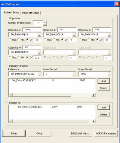
The MOPSO was coded in VBA as a generalized multiobjective solver that can be imported as an add-in to Excel. The MOPSO Solver allows the user to specify up to six objectives to be considered. The user specifies the cell references for the objectives, for the decision variables, and for the constraints. The solver also includes a scripting tool which allows the user to code specific procedures that will be called immediately before the objective functions are evaluated in the MOPSO algorithm. This tool can be used to call external programs or perform computations that cannot be easily made in the spreadsheet. This considerably increases the flexibility of the MOPSO Solver. The MOPSO Solver Interface is presented in Figure 2.

The MOPSO Solver also includes a procedure to incorporate more intelligence in the way the particles move from one iteration to the next. With Equation (3), a particle’s position in any iteration is updated using a randomly defined combination of the particle’s individual best previous position and the position of a nondominated particle selected from the repository. In the case of constrained problems, this combination may yield an infeasible solution. The MOPSO Solver has an option that allows the evaluation of feasible directions for all dimensions, adjusting the velocity given by Equation (3) so that the particle is not allowed to make large steps in directions of increasing infeasibility.

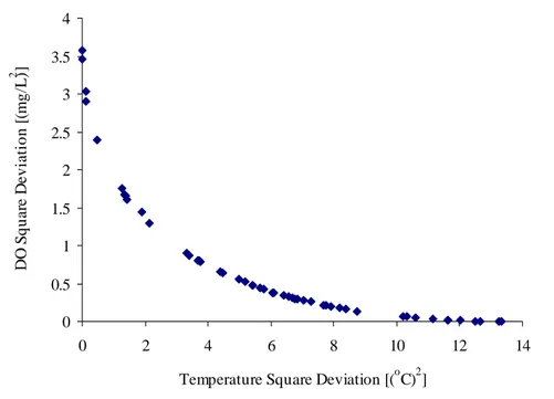
Figure 3 presents the temperature-DO trade-off curve generated by using the MOPSO Solver with 100 particles, a repository size of 50 solutions, and 50 iterations. The processing time was 130 seconds in a PC AMD Athlon™ 64, 2.2 GHz. This problem has two objectives and five decision variables.

0 0.5 1 1.5 2 2.5 3 3.5 4 0 2 4 6 8 10 12 14

Temperature Square Deviation [(oC)2]

D O S q ua re D e vi a ti o n [ (m g/ L ) 2 ]

Figure 3. Temperature-Dissolved Oxygen Trade-off Curve

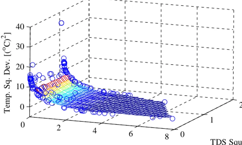
Figure 4 presents a plot of the Pareto surface when minimizing the square deviations from the targets of temperature, DO, and TDS. The MOPSO processing time was 660 seconds with 150 particles, repository size of 150 solutions, and 150 iterations.

The MOPSO Solver also allows the user to define binary decision variables that can be applied to find nondominated solutions when a restriction on the maximum number of ports to be used is desired. For this problem, the user must specify five decision variables representing flows through each port and five binary variables that will determine in each solution whether that port will be used. The flow in each port is the product of the flow decision variable and

its associated binary variable. The user can then include a constraint establishing a limit to the number of ports used, by making the sum of the binary variables to be equal to this limit. This is a very difficult problem to solve, and nonlinear mathematical programming optimization methods will have difficulty finding Pareto optimal solutions.

0 ₂ 4 ₆ 8 0 1 2 0 10 20 30 40 TDS Square Deviation [(mg/L)2] DO Square Deviation [(mg/L)2] Te m p . S q . D ev . [( o C) 2 ]

Figure 4. Temperature-DO-TDS Trade-off Surface 4.1. Procedure to visualize and explore the Pareto set

A procedure was developed to incorporate the preferences of the DM as well as to visualize and explore the Pareto set. First, all Pareto solutions are normalized using a compromise programming approach with a Euclidian norm (L-2 norm). All objectives are placed as vertices equally spaced in a circumference of diameter 1. Let N be the number of objectives. The first objective is arbitrarily assigned to coordinates [0.5,1.0]. The x and y coordinates of the following objectives are given by the following equations:

2 2 ⎟ ⎠ ⎞ ⎜ ⎝ ⎛ − = N π π θ (8)

( )

(

)

(

)

( )

(

)

(

)

Where N is the number of objectives and k = 2,3,..N.

The normalized metrics are calculated for each objective as follows:

( )

[

_{( )}

( ) ( )

_{( )}

]

[

]

Where CP(i,k) is the [0,1] normalized metric of particle i for objective k, and R(i,k) is the value of objective k of particle i in the repository.

The normalized metric for each objective is then used to calculate a new coordinate measured in the diameter corresponding to that objective. The new coordinates are given by:

( )

( )

( )

(

)

( )

( )

( )

(

)

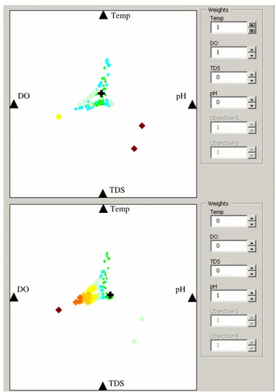
Each particle in the repository now has a (x,y) coordinate for each of the N objectives. The particle is then plotted in the centroid defined by these N points. A weighted average of the normalized metrics is calculated based on weights given by the DM. The DM can change the weights and automatically see the best-compromise Pareto solution, as well as other Pareto solutions with a similar compromise. Figure 5 presents the MOPSO Solver interface with the temperature-DO-TDS-pH trade-off graph for the case of equal weights. Figure 6 presents the same trade-off graph for two other sets of weights, one set with equal weights for temperature and DO and no importance to TDS and pH, and another considering only pH.

Temp

DO _pH

TDS

Temp DO pH TDS Temp DO pH TDS

Figure 6. Temperature-DO-TDS-pH Trade-off Graphs

5. Conclusions

The multiobjective particle swarm optimization algorithm, applied in a model for operation of selective withdrawal structures, proved to be able to find well-distributed nondominated solutions in the objective space. Compared to the goal programming approach of Fontane and Schneider (1994) that only produced single compromise solutions based upon an a priori set of weights, a single run of the MOPSO defined the trade-off regions among the four water quality objectives. Once defined, these trade-off regions can be explored to find a number of compromise solutions based upon a posteriori set of weights.

The graphical procedure proposed in this paper can help decision makers to explore Pareto sets when three or more objectives are considered. The best-compromise solution may be identified as well as subsets of the Pareto set that provide similar compromises.

The MOPSO Solver was found to be very flexible allowing the user to easily conduct many types of analyses. The implementation of the MOPSO Solver as an add-in EXCEL greatly enhances the potential applicability of the approach.

Acknowledgments. The first author of this paper is a sponsored by CNPq,

Brazil.

References

Bohan, J.P. and Grace, J.L. (1973). “Selective Withdrawal from Man-Made Lakes”.

Technical Report H-73-4. U.S. Army Engineer Waterways Experiment Station,

Vicksburg, MS.

Coello Coello, C.A. (2001). “A Short Tutorial on Evolutionary Multiobjective Optimization.” Springer-Verlag, Lect. Notes Comp. Sci. 1993, Berlin, Germany, 21-40.

Coello Coello, C.A., Pulido, G.T., and Lechuga, M.S. (2004). “Handling Multiple Objectives with Particle Swarm Optimization.” IEEE Transactions on

Evolutionary Computation, IEEE, Piscataway, NJ, 8 (3) 256-279.

Elbeltagi, E., Hegazy, T., and Grierson, D. (2005). “Comparison Among Five Evolutionary-based Optimization Algorithms.” Adv. Engineering Informatics, Elsevier, 19 (1) 43-53.

Fonseca, C.M. and Fleming, P.J. (1995). “An Overview of Evolutionary Algorithms in Multiobjective Optimization.” Evolut. Comptn., MIT Press, Cambridge, MA, 3 (1) 1-16.

Fontane, D.G. and Schneider, M.L. (1994). “Description of the Application of Goal Programming for Selective Withdrawal Structure Application.” Proc. 21st Annual ASCE Water Resources Plng. and Mgmt. Division Conf. (Fontane, D.G. and

Tuvel, H.N.,eds.), Denver, CO.

Goicoechea, A., Hansen, D.R., and Duckstein, L. (1982). Multiobjective Decision

Analysis with Engineering and Business Applications. J. Wiley & Sons, New

York, NY, 519 pp.

Jung, B.S. and Karney, B.W. (2006). “Hydraulic Optimization of Transient Protection Devices Using GA and PSO Approaches.” J. Water Resour. Plng. and Mgmt., ASCE, Reston, VA, 132 (1) 44-52.

Kapelan, Z.S., Savic, D.A., and Walters, G.A. (2005). “Optimal Sampling Design Methodologies for Water Distribution Model Calibration.” J. Hydraulic Engrg., ASCE, Reston, VA, 131 (3) 190-200.

Kennedy, J. and Eberhart, R. (1995). “Particle Swarm Optimization.” Proc. 4th IEEE Int. Conf. on Neural Networks, IEEE, Piscataway, NJ, 1942-1948.

Liong, S., Khu, S., and Chan, W. (2001). “Derivation of Pareto Front with Genetic Algorithm and Neural Network.” J. Hydrologic Engrg., ASCE, Reston, VA, 6 (1) 52-61.

McMahon, T.A. and Mein, R.G. (1988). River and Reservoir Yield. Water Resources Publications, Littleton, CO, 368 pp.

Mendes, R., Kennedy, J., and Neves, J. (2004). “The Fully Informed Particle Swarm: Simpler, Maybe Better.” IEEE Transactions on Evolutionary Computation, IEEE, Piscataway, NJ, 8 (3) 204-210.

Miettinen, K. (2001). “Some Methods for Nonlinear Multi-objective Optimization.” Springer-Verlag, Lecture Notes in Computer Science 1993, Berlin, Germany, 1-20.

Muleta, M.K. and Nicklow, J.W. (2005). “Decision Support for Watershed Management Using Evolutionary Algorithms.” J. Water Resour. Plng. and Mgmt., ASCE, Reston, VA, 131 (1) 35-44.

Suen, J., Eheart, J.W., and Herricks, E.E. (2005). “Integrating Ecological Flow Regimes in Water Resources Management Using Multiobjective Analysis.” Proc.

ASCE/EWRI World Water and Envmtl. Resour. Cong., ASCE, Reston, VA.

Tang, Y. and Reed, P.M. (2005). “Multiobjective Tools and Strategies for Calibrating Integrated Models.” Proc. ASCE/EWRI World Water and Envmtl. Resour. Cong., ASCE, Reston, VA.

Zitzler, E. and Thiele, L. (1999). “Multiobjective Evolutionary Algorithms: A Comparative Case Study and the Strength Pareto Approach.” IEEE Transactions