Effect of trends on the estimation of extreme precipitation quantiles
Antonino Cancelliere, Brunella Bonaccorso, Giuseppe RossiDepartment of Civil and Environmental Engineering, University of Catania, Catania (Italy)
Abstract. Estimation of quantiles of hydrological variables, i.e. values corresponding to fixed
non-exceedence probabilities or return periods, is traditionally carried out by fitting a probability distri-bution function to an observed sample under the assumption of stationarity. Recent concerns about potential changes in present and future climate, however have led to challenge the hypothesis of stationary series. Despite several methods have been developed and applied to model non station-ary series, very few studies have addressed the problem of how non stationarity affects the error of estimation of quantiles. In the paper, preliminary analyses regarding how the presence of trend in precipitation series affects the sampling properties of estimated quantiles are illustrated. To this end, sampling properties of precipitation quantiles, namely bias and Mean Squared Error (MSE) are investigated with respect to the size of the estimation sample, assuming a trend in the parame-ters of the underlying distribution. In particular, analytical results are derived for the cases of expo-nential distribution, while more complex cases (e.g. Gumbel distribution) are investigated numeri-cally by simulation. Also the effect of preliminary trend removal is investigated and compared to the case when trend is neglected.
1. Introduction
Probabilistic modeling of hydrological and meteorological variables is generally car-ried out by assuming time series to be stationary. For instance, when the interest lies in es-timating quantiles of hydrological variables, i.e. the values corresponding to fixed non-exceedence probabilities or return periods, the assumption of identically distributed vari-ables is made and consistent estimators are applied, leading to the paradigm that the longer the available sample the better the estimation of quantiles.
Recently, such hypothesis of stationary series is being questioned, also in light of the growing concerns about potential changes in present and future climate. In particular, more and more evidence is produced in literature about the presence of non stationarities in many climatic and hydrological records around the world in the form of trends and/or jumps in the statistics of the series (IPCC, 2007). Regardless of the causes, the presence of non stationarities in the available sample requires to dramatically modify the procedures for estimating probabilistic properties of hydrological time series. Several methods have been developed and applied to model non stationary series including stochastic modelling (e.g. North, 1980; Kottegoda et al., 2007), Bayesan approaches (e.g. Perreault et al., 2000a, b; Renard et al., 2006), likelihood based approaches (e.g. Strupczewski et al., 2001) as well as pooled frequency analysis (e.g. Cunderlick and Burn, 2003). Nonetheless, very few studies have addressed the problem of how non stationarity affects the error of estimation of quantiles.
Indeed, in a non stationary setting, the statement “the longer the sample, the better the estimation” obviously does not hold anymore. On the other hand, one may expect that too short a sample also should lead to larger errors of estimation. Therefore, the existence of an optimal sample size, where optimal refers to the sampling properties of the estimators, can be postulated.
ing it from the series for estimating the distribution parameters, leads to an improved esti-mation of quantiles. Alternatively, the estiesti-mation of trend parameters can be included within the estimation of the parameters of the distribution, for instance by adopting Maxi-mum Likelihood (Strupczewski et al, 2001). Nonetheless, due to the uncertainties related to the choice of the correct parametric form of the trend, as well as to the sampling vari-ability related to the estimation of its parameters, the estimated quantiles may not necessar-ily be affected by a smaller error with respect to the case when the trend is neglected. Thus the analyst is left with the dilemma whether to detrend a potential unknown trend, or to ne-glect it. Traditionally, tests to assess the statistical significance of an observed trend are applied (e.g. Student’s t-test for linear trends, Mann-Kendall τ-test, etc.) and the decision as to whether detrend or not is made based on the outcome of such tests.
In the paper the sampling properties of precipitation quantiles, namely bias and Mean Squared Error (MSE) are investigated in the case of precipitation series affected by a trend component in the mean. In particular, analytical expressions of bias and MSE of estimation of precipitation quantiles are derived for the case of exponential distributed series affected by a linear trend. Sampling properties of a fixed quantile are also analyzed for the case of Gumbel distributed series characterized either by a linear or a parabolic trend in the mean based on Monte Carlo simulations. In what follows we will not consider the uncertainty re-lated to the unknown functional form of the distribution, but we will limit our analysis only to the sampling variability due to the estimation of parameters, when the available sample is affected by trend.
Finally, the effect of preliminary trend estimation and removal is investigated numeri-cally by simulation and compared to the case when trend is neglected.
2. Effects of trends on sampling properties of quantiles
In order to assess the effects of trends on sampling properties of quantiles, first the case of exponentially distributed variables affected by linear trend in the mean has been investi-gated, since it enables a relatively simple analytical solution that is useful to frame the problem. In particular, bias and Mean Square Error of Estimation (MSE) have been com-puted as a function of the length of the available sample used for estimation and of the trend characteristics. Then more complex cases have been tackled by simulation, including different distributions and non linear trends.
Let us consider a random variable affected by a trend in the mean which, without loss of generality we will model as:
(1)
where g(t) is a trend function and is a residual independently and identically distributed according to some distribution
Taking expectations from Eq. (1), it follows:
(2)
Previous equation reflects the fact that the mean changes with time, and so will the dis-tribution of Xt. As a consequence, the q-quantile, i.e. the value corresponding to a non-exceedence probability equal to q, will depend on time as well. In the present investigation we will concentrate our attention to the case t=n+1, having assumed observations up to time n (present) and considering that we may be interested in the quantile one time step
ahead in the future. However, it may be worthwhile to note that extension to the generic case t=n+m, with m= 1, 2,… is straightforward.
More specifically, we will consider the following (non stationary) time series,
t=…0,1,2,…:
(3)
where b is the parameter of the linear trend in the mean and is a residual independently and identically exponential distributed, with probability density function (pdf) and cumula-tive distribution function (cdf) respeccumula-tively:
(4) (5)
Note that, in this case, and . Then the (unknown) true
q-quantile at time n +1 is:
(6)
On the other hand, without prior removal of the unknown trend, the corresponding maximum Likelihood (ML) estimated quantile based on an available sample x1, x2, …, xn. from the process represented by Eq. (3) will be:
(7)
where is the sample mean of the available sample.
The sampling variability of can be characterized by investigating the properties of the difference (error) between the true and the estimated quantiles, namely of the following random variable:
(8)
Although in principle one may be interested to the distribution of D, generally, the first two moments of the error provide enough information to characterize the sampling vari-ability of the estimator , since they allow to compute the bias and the Mean Squared Er-ror (MSE) of estimation, as:
(9) (10) Combining Eqs. (6), (7) and (8), Eq. (8) can be rewritten as:
(11)
Therefore the bias of estimation of is:
(12) In a similar fashion the variance of D can be expressed as:
(13)
Therefore replacing Eq. (12) and Eq. (13) into Eq. (10), one gets the MSE of estimation of as:
(14) Taking into account Eq. (3), the sample mean is by definition:
(15)
whose expected value and variance are respectively and
.
Therefore, after some algebra, Eqs. (12) and (14) become:
(16) (17)
Eqs. (16) and (17) enable to characterize the sampling variability of the q-quantile for an exponential process with a linear trend in the mean. In particular, Eq. (16) indi-cates that bias exhibits a linear dependence on n and b. On the other hand, MSE (Eq. (17)) has a non linear dependence on n and b.
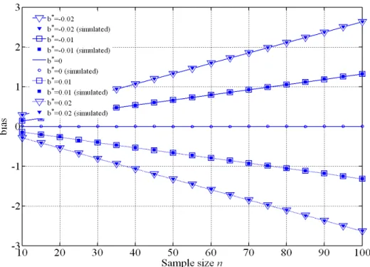
In Figure 1 and Figure 2, respectively the bias (Eq. 16) and Root Mean Square Error, RMSE (square root of Eq. 17) of 99% quantile are shown as a function of the length of the available sample n and of the slope of the trend, the latter expressed as ratio to the standard deviation of the process λ, namely b*=b/λ. In the same plots, the corresponding values of bias and RMSE obtained by Monte Carlo simulation are plotted as well. More specifically, first, 5000 series of n values are sampled by generation from an exponential distribution with λ=1 and a trend component is added to each series according to Eq. (3). The simu-lated 99% quantiles are computed by first adapting an exponential distribution to each of the 5000 generated samples by means of ML method. Then the mean of the difference and of the squared difference between the estimated and the “true” 99% quantiles are com-puted, yielding an estimate of the bias and MSE.
The plots indicate very good agreement between the analytical values from Eqs. (16) and (17) and those computed by simulation, thus confirming the validity of the derived analytical expressions. As it can be observed from Figure 1, the larger the sample size n, the more bias values diverge from zero, with positive bias for b*<0 and negative otherwise. Furthermore, for a fixed sample size, the difference from zero enlarges as the absolute value of b* increases. This is expected due to the fact that as more past values are included in the estimation sample, the estimate of the mean and standard deviation will be affected by increasing error due to the trend.
However, as it can be observed from Figure 2, the RMSE exhibits a rather different be-haviour, since, as sample size n increases, the RMSE first decreases and then increases again. Therefore, a minimum value of RMSE can be determined for each considered slope
b*≠0 corresponding to a given sample size. In particular, such a sample size reduces as the absolute values of b* increases.
Figure 1. Analytical and simulated bias of estimation of 99% quantile in the case of exponential distributed
series affected by a linear trend with different slope parameter b*
Figure 2. Analytical and simulated RMSE of estimation of 99% quantile in the case of exponential
distrib-uted series affected by a linear trend with different slope parameter b*
Although in principle, analytical expressions of the sampling properties can be derived for different probability distributions and trend components in the underlying series, in what follows only results related to numerical simulations are reported. In particular bias
and RMSE of 99% quantile have been computed from randomly generated samples of dif-ferent size n distributed according to a Gumbel distribution and affected either by a linear or non linear trend, following a Monte Carlo simulation similar to that applied for the ex-ponential case.
In particular, Equation (3) has been applied for the linear trend case, while in the case of non linear trend the following expression has been considered:
(18)
where , namely:
(19) (20)
For the sake of comparing the results related to linear and non linear trends, the pa-rameter a has been chosen in such a way that the change in the mean between time t=1 and t=n+1 is the same in the two cases, namely a=b/(n+1).
The “true” 99% quantile at time t=n+1 is computed as:
, where , since we have assumed ,
and .
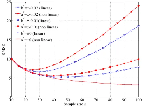
In Figure 3, the values of RMSE obtained by simulation both for the linear trend case (no filled markers) and non linear trend case (filled markers) are plotted versus the sample size for different slopes expressed as ratio to the standard deviation s. Again, it can be in-ferred that RMSE as a function of the sample size n exhibit a minimum which depends on the slope of the trend. Furthermore, it is worth observing that non linear trends yield greater RMSE values with respect to the equivalent linear trends.
Figure 3. RMSE of estimation of 99% precipitation quantiles computed from simulation in the case of
Gumbel distributed series affected by a linear (no filled markers) and non linear trend (filled markers) with different slope parameter
3. Effect of trend removal on sampling properties of quantiles
In this section the effect of preliminary trend removal is numerically investigated in or-der to assess to which extent and unor-der what conditions detrending leads to an improved estimation of precipitation quantiles, compared to the case when trend is neglected. In principle, if the true trend would be known, detrending would obviously always lead to an improved estimation of the quantiles at time t=n+1, or in general of the whole distribution. However, this is hardly the case, since in general the true trend is unknown, both in terms of its functional form as well as of its parameters. Thus, trend estimation is generally af-fected by some degree of uncertainty and therefore, its removal prior to fitting a probability distribution to an observed sample does not necessarily leads to improved (at least in bias and MSE sense) estimation of quantiles.
In order to assess the effect of either detrending or not a non linear time series, the simulation analysis described in Par. 2 has been repeated considering Gumbel variates af-fected by linear trend. For each generated samples the parameters of the linear trend have been estimated by means of Least Squares method and for each series the trend has been removed, prior to the estimation of the parameters of the Gumbel distribution by ML. More specifically, with reference to a generic generated sample of length n x1, x2, …, xn, the intercept a and the slope b of the linear trend have been estimated by:
(21) (22)
where . Then, the detrended sample is given by:
(23) and the corresponding q-quantile at time t=n+1 can be expressed as:
(24)
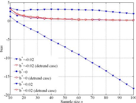
where u’ and α’ are the parameters of the Gumbel distribution fitted to the detrend sample. In Figure 4 and Figure 5 respectively the bias and RMSE of estimation of q=99% quan-tile from a Gumbel distribution with variance s2=100 mm are reported versus the sample size n, having assumed a linear trend with dimensionless slope b*=b/s =-0.02 in the first
moment of the distribution. For the sake of reference, also the case b*=0 is plotted (station-ary series).
From Figure 4 it can be inferred that, in terms of bias, removing the trend always leads to an improved estimation of the q-quantile. In particular, for the detrending case, the esti-mator is unbiased since bias values are close to zero regardless the sample size n.
Conversely, in the case of RMSE (Figure 5), the comparison with the detrending case, reveals that detrending leads to a reduced MSE only for sample sizes above a given value. In particular, detrending leads to a higher RMSE when the sample size n is smaller than 30 for a dimensionless slope b*=b/s =-0.02. Finally, the comparison with the case b*=0,
therefore, detrending erroneously a stationary series introduces errors in the estimation of quantile.
Although the above results cannot find immediate practical application, since the true trend is unknown and therefore a decision on whether to detrend or not cannot be based on Figure 4 and 5, nonetheless, they indicate that detrending may adversely affect the estima-tion of quantiles in some cases, and therefore care must be taken.
Figure 4. Comparison between bias of estimation of 99% quantile in the case of Gumbel distributed series,
obtained either by removing (detrend case) or neglecting the linear trend with different slope parameter b*
Figure 5. Comparison between RMSE of estimation of 99% quantile in the case of Gumbel distributed
4. Conclusions
In the present paper the sampling properties of precipitation quantiles have been inves-tigated for the case of non stationary (namely affected by a trend in the mean) series.
In particular, analytical expressions of bias and RMSE of estimation of a fixed quantile have been derived for the case of exponential distributed precipitation series affected by a linear trend and validated by Monte Carlo simulations. Results indicate that bias values di-verge from zero as either sample size or trend slope increase, while RMSE first decreases until a minimum value is reached corresponding to a specific sample size and then in-creases again.
Similar results are also obtained numerically for the case of Gumbel distributed pre-cipitation series affected either by a linear and non linear trend. This seems to confirm that when non stationarities (at least in the form of trends in the mean values) are present, longer samples do not necessarily reduce the error of estimation of quantiles. Furthermore, the presence of a non linear trend yields larger RMSE values with respect to the linear trend case.
Finally, preliminary results as to whether detrending a suspected non stationary series can lead to more reliable estimates compared to the do-nothing alternative, have been shown with respect to the possibility to reduce the error of estimation of estimated quan-tile. In particular, simulation experiments have shown that detrending an unknown trend can lead to higher error of estimation when the sample size n is smaller than a given value, which depends on the sample size as well as on the slope of the true unknown trend. This finds an explanation because of the added uncertainty related to estimating the unknown trend, which, especially for smaller samples and smaller slopes may introduce substantial errors.
The overall conclusion of the paper is that knowledge of the sampling properties of ex-treme precipitation quantiles is particularly important when the underlying precipitation se-ries is suspected to be affected by non stationarities in the form of trends. Indeed, in this case, the estimation is not consistent and an optimal (in RMSE sense) sample size exists. Furthermore, for particular combinations of trend slope and sample length, removing a suspected trend does not necessarily lead to an improved estimation of quantiles.
Ongoing research is oriented to extend the present analysis by computing the sampling properties of quantiles as a function of the estimated trend parameter.
Acknowledgements. The financial support of the national project MIUR-PRIN 2007,
“Drought indicators and models for the definition of triggering levels for measures to pre-vent water emergencies in water supply systems” (20075WFE7P) is gratefully acknowl-edged.
References
Cunderlik, J.M. and Burn, D.H. (2003). Non-stationary pooled flood frequency analysis. Journal of Hydrol-ogy, 276:210-223.
IPCC, (2007). Climate Change 2007: Synthesis Report. Contribution of Working Groups I, II and III to the Fourth Assessment Report of the Intergovernmental Panel on Climate Change, Core Writing Team, Pachauri, R.K and Reisinger, A. (eds.). IPCC, Geneva, Switzerland, 104 pp.
Kottegoda, N.T., Natale, L. and Raiteri, E. (2007). Gibbs sampling of climatic trend and periodicities. Journal of hydrology, 339: 54-64.
North, M., (1980). Time-dependent stochastic model of floods. Journal of the Hydraulics Division, ASCE 106 (HY5), 649-665.
Perreault, L., Bernier, J.; Bobee, B., Parent, E. (2000a). Bayesian change-point analysis in hydrometeorologi-cal time series. Part 1. The normal model revised. Journal of Hydrology, 235: 221-241.
Perreault, L., Bernier, J.; Bobee, B., Parent, E. (2000b). Bayesian change-point analysis in hydrometeoro-logical time series. Part 2. Comparison of change-point models and forecasting. Journal of Hydrology, 235: 242-263.
Renard, B., Lang, M. and Bois, P. (2006). Statistical analysis of extreme events in a non-stationary context via a Bayesian framework: case study with peak-over-threshold data. Stochastic Environamental Research and Risk Assessment, 21: 97-112.
Strupczewski, W.G., Singh, V.P. and Feluch, W. (2001). Non-stationary approach to at-site flood frequenvy modelling I. Maximum likelihood estimation. Journal of Hydrology, 248: 123-142.