How to get 3-D accuracy with a 2-D stream-aquifer interaction model (or "The turning resistance factor in river seepage")

How to get 3-D accuracy with a 2-D stream-aquifer interaction model

(or “The Turning Resistance Factor in River Seepage”)

Hubert J. Morel-Seytoux

Hydroprose Consulting International, 57 Selby Lane, Atherton, CA 94027-3926

Abstract. Close to a river the traditional groundwater Dupuit assumption of horizontal flow does not hold. In order to treat the problem accurately one would need to use a 3-dimensional numerical model with small cells in the vicinity of the river. Presented here is an analytic approximate way to avoid this extra complication and still describe accurately the exchange flow between the stream and the aquifer.

1. Raison d’être for this investigation

In the vicinity of a river (or canal) reach the Dupuit-Forchheimer (D-F) assumption does not hold. In order to treat the problem accurately one would need to use a

3-dimensional model with small cells in the vicinity of the reach. Given the usually small horizontal spatial extent of the reach footprint, one may legitimately wonder if there might not be an approximate yet adequate way to avoid this extra complication?

2. Previous Work

To alleviate that difficulty it has been proposed to link a vertical analytical 2-dimensional solution to the numerical horizontal 2-2-dimensional model. A “reach

transmissivity” is defined so that the exchange discharge Q (volume per unit time) would be given by the expression:

€

Q = ΓΔH (1)

where ΔH is the head difference between the reach and the aquifer at a finite distance from

the reach. Eq. (1) is an integrated form of Darcy’s law over a finite distance which accounts for the geometrical character of the flow path. How is Γ determined?

It can be done analytically or numerically. 3. Analytical Approach

Figure 1 shows schematically such a flow path. Clearly in the vicinity of the reach bottom the flow is primarily vertical. Only as a distance xfar is reached does the flow

become essentially horizontal. In the 1940’s and 50’s, it was assumed for simplicity, that the stream had no width and fully penetrated the aquifer. With the assumption of full penetration no resistance is accounted for the difficulty the flow encounters to change direction from a vertical to a horizontal one. The purpose of this investigation is to compare the results of an analytical approach for this added resistance “turning” factor with those obtained with: (a) the assumption of full penetration and (b) a Finite Difference grid.

4. A Finite Difference Dimensionless Conductance

The simplest grid one can conceive would be one that has one cell below the reach horizontal bed and of width the actual wetted perimeter. Figure 2 displays the

74

cross-section and half the cell is shown. Next to that cell to the right is another cell of width 2 Δxfar with center at point C where the head is HC. Beyond that cell further to the

right the D-F assumption applies. Using Darcy’s law and the principle of continuity the conductance is expressed as:

€ ΓFD= 1 e_B W_p + W_p 2e_B + Δx_far e_B           (2)

o

x

y

D

y

y

x

e

e

-x

Figure 1. River or canal cross-section

The seepage flow from half the reach is then given as:

€

Q = KLΓFD(HR− HC) = KLΓFDΔHfar (3) where ΔHfar is the head drop between the reach and the cell center located at a distance

from the reach equal to Δxfar.

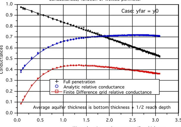
Figure 3 shows a comparison of the Analytical and the Finite Difference

conductances, both expressed relative to that of Full Penetration. It is clear that the Finite Difference approach greatly underestimates the seepage. To get better accuracy with this approach one would have to have a grid that follows the contour of the cross-section and thus use a 3-dimensional model. However this is precisely what one wants to avoid.

Water depth cell centers HR HA _HC Wp/2 _DXfar aquifer thickness axis of symmetry

Figure 2. Finite Difference grid used to estimate stream-aquifer conductance 5. Practical Use of the Results of the Analytical Approach

Now how are the results shown in Figure 3 to be used? Take the ratio ΓAN/ΓFP, displayed in Figure 3, and call it Γr the “turning factor”. It is the factor that needs to multiply the full penetration conductance to account for the added turning resistance to flow and for the difference in areas through which the flow moves. This is a function of the ratio WP/e and similarly is Δxfar, shown on Figure 4.

The exchange discharge from one side is then defined as:

€

Q = KLΓrΓFPΔHfar (4)

where ΔHfar is the horizontal head difference between the canal perimeter and the far

section at

€

Δx_far = (x_far− B) .

Consider a simple numerical example. Take a bottom aquifer thickness eB of 10.0 m, a depth of 3.0, thus

€

e = 11.50, and a wetted perimeter of canal of 12.25 m.

Then WP/

€

e

€

Γ_FP = 0.82 and

€

Γ_r = 0.67. Assume a hydraulic conductivity of 10.0 m/day, and a reach length of 1 km. Then the discharge from one side will be:

Q = 10x1000x0.67x0.82x

€

ΔH_far= 5,494x

€

ΔH_far cubic meters/day where

€

ΔH_far is the drop of head, also measured in units of meters, over the distance

€

Δx_far = (x_far− B) = 1.23x 11.50= 14.1 meters (using Figure 4). Had one assumed full penetration the discharge would have been overestimated as 8,200xΔH_far cubic meters/day.

76 0.0 0.5 1.0 1.5 2.0 2.5 3.0 3.5 0.0 0.1 0.2 0.3 0.4 0.5 0.6 0.7 0.8 0.9 1.0

Wetted perimeter/average aquifer thickness Conductances, function of wetted perimeter

Full penetration

Analytic relative conductance

Finite Difference grid relative conductance

Case: yfar = y0

Average aquifer thickness is bottom thickness + 1/2 reach depth

Figure 3 Comparison of different estimations of stream aquifer conductance. Case: yfar = y0

0.0 0.5 1.0 1.5 2.0 2.5 3.0 3.5 0.0 0.1 0.2 0.3 0.4 0.5 0.6 0.7 0.8 0.9 1.0 1.0 1.1 1.2 1.3 1.4 1.5 1.6 1.7 1.8 1.9 2.0

Wetted perimeter/average aquifer thickness Normalized water depth and distance to far section

Normalized reach water depth Normalized distance to far section Case: yfar = y0

Average aquifer thickness is bottom thickness + 1/2 reach depth

One may rewrite Eq.(4) in the form:

€

Q = KLΓ_r{WP / e } e

[Δx_far{WP / e }]ΔHfar (5) where the dependence of the variables on the ratio WP/

€

e

Had we used the Finite Difference estimation the discharge would have been: Q = (0.44 /0.67)x5,494x

€

ΔH_far= 3,608x

€

ΔH_far Application in Numerical Groundwater Modeling

With the proposed approach one can still formally assume full penetration provided that the discharge going into the cell with center at point C (see Figure 2) be given by Eq.(5).

Eq.(5) has the inconvenience that its direct application would require that distance from reach center to cell center be precisely xfar. Now typically in large scale groundwater

models the cells are considerably wider than the reaches. Let then

€

Δx_RC be the distance between the edge of the reach and the cell center and let

€

ΔH_RC = H_R− H_C be the head drop between them. Again using Darcy’s law and the principle of continuity one obtains for the conductance and the discharge in this case:

€ Q = KL 1 [1+ (1 Γ_r − 1) Δx_far Δx_RC]               ( e Δx_RC)ΔHRC (6)

In most groundwater models to calculate the river seepage the multiplier of the head difference would be treated as a constant. However it is clear from Eq.(6) that it would be very easy to account for the change in the reach transmissivity as a result of rise or fall of the stage in the reach since the relative conductance is a function of the wetted perimeter.

The great advantage of Eq.(6) is that it is no longer necessary to have a fine grid size in the vicinity of the reach to calculate accurately the seepage from the reach.

Case of clogging at the reach bottom

For simplicity let us define the relative dimensionless conductance in Eq. (6) as:

Γ_rRC = 1 [1+ ( 1 Γ_r − 1) Δxfar Δx_RC ]               (7)

78

If there is clogging at the reach bottom with a hydraulic conductivity Kc over a thickness ec

then again simple algebra combined with mass conservation will yield a correction for the expression of the discharge:

€ Q = LK 1 1+ ( K K_c)( e_c W_p)( e Δx_RC)ΓrRC               Γ_rRC( e Δx_RC)ΔHRC (8)

Limitations of the Study

One limitation, among others, is the fact that the results of Figures 3 and 4 depend on the shape of the river cross-section. Figure 5 shows the shape of the reach cross-section for a particular value of the ratio of wetted perimeter over average aquifer thickness. It is a reasonable shape. -4.0 -3.5 -3.0 -2.5 -2.0 -1.5 -1.0 -0.5 0.0 0.5 1.0 1.5 2.0 2.5 3.0 3.5 4.0 -3.0 -2.5 -2.0 -1.5 -1.0 -0.5 0.0

Horizontal distance from center of reach cross-section Depth/average aquifer thickness = 0.242

Wetted perimeter/average aquifer thickness = 0.984 Depth = 2.963 Half top width = 3.625

Depth as a function of distance from center

Figure 5. Cross section when depth of water is 2.42 units of length and aquifer thickness is 10 Conclusions

A potentially very practical tool has been suggested for a numerically efficient and adequately accurate 2-dimensional alternative to a full detailed 3-dimensional modeling. There is little need for a detailed grid description of the reach cross-section. In fact the full penetration assumption can be used provided that the flow across the reach vertical boundary be corrected by the turning factor. What has been quantitatively

demonstrated is that neither the traditional assumption of full penetration nor the use of a typical Finite Difference grid model will provide adequately accurate results. However it must be emphasized that it is not necessary to proceed to a 3-dimensional model to improve accuracy but rather correct the manner in which the seepage discharge is calculated while conserving a typical Finite Difference grid.