Estimating the Spatial Distribution of a First-Order Solute Decay
Constant in Groundwater Systems
Ryan T. Bailey1 and Domenico A. Baù
Department of Civil and Environmental Engineering, Colorado State University
Abstract. Numerical models capable of simulating solute reactive transport in groundwater
systems are often used as tools to assess the state of contaminated aquifer systems. Accurately simulating the fate and transport of solutes, however, is often hindered by a lack of information regarding the chemical reactions parameters that govern the fate of the solute. Furthermore, field and laboratory methods used to determine these parameters are often labor- and resource-intensive, and often cannot be translated to numerical models due to differences in scale, especially for large-scale aquifer systems. In this study, we employ a steady-state Ensemble Kalman Filter (EnKF), a data assimilation algorithm, to provide improved estimates of a spatially-variable first-order rate constant λ through assimilation of solute concentration C measurement data into reactive transport simulation results. The numerical model establishes correlation between λ and the calculated C values throughout the model domain. This correlation, along with model results and measured C values from a reference field, are used by the EnKF to correct model-calculated C values as well as
λ in adjacent locations in the model domain. The methodology is applied in a steady-state, synthetic
aquifer system in which a contaminant is leached to the saturated zone and undergoes advection, dispersion, and first-order decay in the aquifer system. Uncertainty regarding the hydraulic
conductivity of the aquifer is also included. Results from all simulations show that the filter scheme is successful in conditioning the λ ensemble to a reference λ field.
1. Introduction
Physically-based, distributed numerical contaminant transport models are being used with increasing frequency in an attempt to accurately assess the fate and transport of solutes in contaminated aquifer systems. The performance of these models, however, is dependent on the values assigned to the input parameters required for simulation, the magnitude and spatial distribution of which are often not known with certainty.
Consequently, contaminant transport model simulations often fail to capture the patterns of solute concentration within the true aquifer system. Inadequate knowledge regarding contaminant transport parameters is especially acute in the case of reaction rate constants, which are known to vary log-normally [Parkin and Robinson, 1989; McNab and Dooher, 1998], much like hydraulic conductivity, and yet are often assigned a uniform value across the entire model domain [e.g., Frind et al., 1990].
In an effort to provide more reliable information concerning both the parameters and variables of a given dynamic system, data assimilation (DA) methods have been used with success in hydrologic applications [e.g., Liu and Gupta, 2007]. Among the available DA schemes, the Kalman Filter (KF) [Kalman, 1960], designed for systems of linear dynamics, has been used extensively in modeling studies to merge real-world measurement data with
1 Department of Civil and Environmental Engineering Colorado State University
Fort Collins, CO 80523-1372 Tel: (970) 491-5387
model results to provide optimal estimates of system variables and parameters. In recent years, DA schemes have also been used in contaminant transport studies to estimate the distribution of solute concentration in aquifer systems [e.g., Zou and Parr, 1995; Chang
and Latif, 2010], dispersivity values [Liu et al., 2008], and sorption rates [Vugrin et al.,
2007]. None, however, have addressed the spatial heterogeneity of chemical reaction rates. In this paper, we present results of using a DA scheme, the Ensemble Kalman Filter (EnKF) to estimate the spatial distribution of a first-order kinetic rate constant λ that governs the decay of a solute with an aquifer system. Using an ensemble of spatially heterogeneous λ fields and the associated ensemble of model-simulated solute
concentration C fields, measurements of C from a reference state are used to provide (i) an updated estimate of the C ensemble that approaches the reference C field, and (ii) an updated estimate of the λ ensemble that approaches the reference λ field. The method is demonstrated using a synthetic two-dimensional flow and transport simulation, in which a solute is leached to the aquifer system with recharge and undergoes advection, dispersion, and first-order decay. An ensemble of hydraulic conductivity K fields was used to account for uncertainty in the flow field. Sensitivity of the update algorithm to (i) number of C measurement data assimilated and (ii) error of the C measurement data are presented.
2. Theory of Data Assimilation
Data assimilation is a process whereby measurement data are incorporated into model simulation results to provide a corrected estimate of the system state. Following the basic framework of Bayesian statistics, the degree of correction depends on the uncertainty associated with both the simulation results and the measurement data. The data
assimilation algorithm used in this study is based on the Kalman Filter method, which has been used extensively in hydrologic applications, particularly groundwater modeling studies [e.g., Camporese et al., 2009]. The Ensemble Kalman Filter (EnKF) [Evensen, 1994] is an extension of the Kalman Filter method for application to large-variable systems, and uses an ensemble of model realizations to define the error statistics of the predicted system state.
The basic form of the algorithm follows a prediction-correction cycle, with corrections made to the system state whenever measurement data are available for assimilation. The prediction step involves forecasting an ensemble of model states Xk at time k forward in
time based on the solution to the groundwater model Φ, system parameters, P, initial conditions I, forcing terms q, and boundary conditions b, generating the predicted state
Xpk+1, where the p superscript represents prediction:
(1) In groundwater modeling applications, each realization of the ensemble is run forward in time using a different set of system parameters, P, thus creating an ensemble of model states in which model results at a given location in the model domain are spread over a range of values, signifying the uncertainty in the system prediction. At time k + 1 a set of measurements zk+1 (e.g., hydraulic head, solute concentration) is collected, perturbed to
account for measurement error, and assimilated into the system state Xpk+1 according to the
following correction equation, to produce a corrected system state Xc k+1:
(2) The matrix dk+1 hold the perturbed measurements, and the matrix H contains binary
constants (0 or 1) that map model results at measurement locations to actual
measurements, creating a residual at measurement locations between the predicted and actual value. The matrix K is termed the Kalman Gain matrix, and has the following structure:
(3)
where Cf is the forecast error covariance matrix associated with the model forecast
Xfk+1 and R is the measurement error covariance matrix associated with the perturbed
measurements d. The formulation of K performs the dual role of (1) spreading information from measurement locations to regions between these locations, allowing the measurement information to correct predicted values throughout the model domain, and (2) acts as a weighting term that scales the correction terms according to model and measurement error. As R approaches zero, signifying low error in the measurement data, the influence of K increases and the residual is weighted more heavily. The model forecast values thus approach the measurement values. In contrast, as Cf approaches 0, signifying relative agreement among the model realizations, the influence of K decreases, and the residual is weighted less heavily. The model forecast values thus receive little to no correction from the measurement data.
3. Parameter Estimation using Data Assimilation
Estimation of the parameter λ in a chemically reactive aquifer environment is performed using the process described in Figure 1. An ensemble of random log spatial parameter fields, with each field encompassing the model domain, is created using a sequential Gaussian simulation algorithm called SKSIM [Baú and Mayer, 2008] using the specified mean µ, standard deviation σ, and correlation length l. The generated ensemble of parameter fields is then used in a numerical contaminant transport model to generate an ensemble of solute concentration C fields, with a value of C calculated for each model grid cell. For this study, the modeling code RT3D [Clement, 1997], which simulates reactive transport of multiple species in saturated three-dimensional aquifer systems, is employed as the numerical contaminant transport model. In parallel, a reference λ field and
associated numerically-calculated C field are established, from which measurement data are collected and against which updated λ and C fields will be compared to test the efficiency of the methodology.
The predicted λ and C ensembles populate the predicted system state matrix Xp
k+1 (see
Equation (2)), the correlation between λ and C is established in the matrix Cf, and
measurement data from selected grid cells of the reference C field are collected, perturbed with a specified coefficient of variation to mimic error in the measurement data, and placed in the matrix d. These matrices are then used in the EnKF update routine to correct the predicted λ and C ensembles, with the ability of the C measurement data to correct the λ values dependent on the strength of correlation between λ and C established by the contaminant transport model. In the scenario used in this paper, this correlation is
diminished due to uncertainty in the spatially-variable K of the aquifer, which is simulated using an ensemble of K fields in the flow model to establish an ensemble of hydraulic head fields that are used to obtain the advection field used in the contaminant transport model.
For any given grid cell in the model domain, the C value is a result of both K (influences the advection of the solute with the flow of groundwater) and λ.
Figure 1. Process of estimating system parameters using
The performance of the update routine to bring the λ ensemble into conformity with the true aquifer system from which the C measurement data were collected is analyzed by comparing the updated ensemble to the reference state viathe performance parameters AE (Absolute Error) and AEP (Absolute Error Precision):
(4)
(5) The AE term compares the model values to the reference value at each location in the model domain, with a lower value signifying a closer approximation to the reference state; the AEP term compares the model values to the ensemble mean at each location, providing a measure of the spread of the values, with a lower value signifying a smaller spread of ensemble values. Hence, AE determines if the updated state approaches the reference state, and AEP determines the confidence in this estimate.
4. Model Prediction
In the considered tests, the model domain is 510 m west-east and 310 m north-south with 10 m by 10 m grid cells. The aquifer has a saturated thickness of 10 m, and the flow field has constant-head boundaries of 100 m and 95 m along the north and south edges of the aquifer, respectively. A constant recharge of 0.005 m day-1 is assigned to each grid cell. An ensemble of K fields is generated using µlog K -3.94, σ = 0.274, and l = 250 m, resulting
in K values ranging from 0.864 m day-1 to 118.3 m day-1. For the transport simulation, solute with concentration of 1000 mg L-1 is leached to each grid cell with the recharge water. Each realization is run to 1000 days to achieve steady-state conditions. The
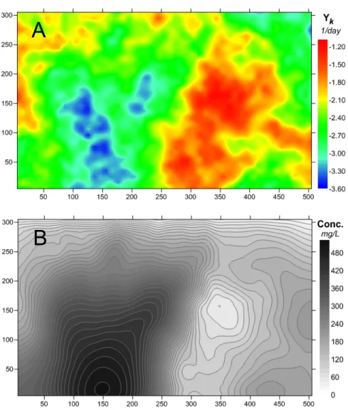
reference λ field shown in Figure 2A shows regions of high reactivity (red), medium activity (green-yellow), and low reactivity (blue). The corresponding reference C field, simulated using RT3D, has high solute concentrations in regions of low λ values, and vice versa, since high reaction rates yields a high consumption of the solute over time. The AE and AEP values for the λ forecast ensemble are 0.697 and 0.574, respectively.
Figure 2. (A) Reference λ field and (B) corresponding reference C field.
5. Model Update
The C and λ forecast ensembles were updated using C measurements from locations shown in Figure 3. Update scenarios were considered where (i) 2 C measurements were assimilated (shown in blue in Figure 3), (ii) 8 C measurements were assimilated (the northern-most 4 and southern-most 4 measurements shown in Figure 3), and (iii) 20 C measurements were assimilated (shown in red in Figure 3). For scenario (ii), an additional three scenarios were considered where coefficient of variation (CV) values of 0.10, 0.30, and 0.50 were assigned to the C measurement data collected from the reference state.
A
Figure 3. Conceptual model of the synthetic aquifer, with groundwater
flowing from north to south. Green and red dots designate grid cells from where C measurement data are collected for assimilation in the case of (i) two measurements and (ii) 20 measurements, respectively. For the case of 8 measurements, the northern-most four and southern-most four measurements are used.
5.1 Sensitivity Analysis: Number of C Data
The results of updating the λ ensemble using (i) 2 C measurements, (ii) 8 C measurements, and (iii) 20 C measurements are shown in Figures 4A, 4B, and 4C, respectively. As can be seen, assimilating more C measurements brings the mean of the λ ensemble more into conformity with the reference λ field shown in Figure 2A. The AE values for the three scenarios are 0.574, 0.467, and 0.457, respectively, as compared to the forecast value of 0.697.
5.2 Sensitivity Analysis: Measurement Error of C Data
Typically, measurement data collected during field sampling events contain error, i.e., they do not provide the exact variable value that exists in the true aquifer system. To incorporate measurement error, each C measurement data value was assigned a coefficient of variation value to provide an ensemble of measurement values to be used in the EnKF update scheme. For example, if the C measurement value is 100.0 mg L-1 and the CV of the measurement value is specified to be 0.10, then the ensemble of measurement values range from approximately 75.0 to 125.0 mg L-1, with the majority of values between 90.0 and 110.0 mg L-1. To analyze the sensitivity of the update routine to measurement errors, three additional update scenarios were run using CV values of 0.10, 0.30, and 0.50 for the 8 measurement values collected from the reference state.
Figure 4. Mean of the updated λ ensemble at every grid cell when (A) 2 (B) 8,
and (C) 20 C measurements are assimilated.
The results of the three scenarios are shown in Figure 5, with the difference between the mean of the updated λ ensemble and the λ reference state (see Figure 2A) becoming greater for a higher CV value. The AE values for the three scenarios are 0.474, 0.512, and
A
B
0.552, respectively, as compared to the value of 0.467 when no measurement error is assigned to the 8 C measurements (see Section 4.1).
Figure 5. Mean of the updated λ ensemble at every grid cell when CV values of
(A) 0.10 (B) 0.30, and (C) 0.50 are assigned to the 8 C measurements.
A
B
6. Conclusions
The Ensemble Kalman Filter (EnKF), a statistical data assimilation routine that merges uncertain, model-produced values with measurement data, was implemented and evaluated in its ability to condition first-order rate constant (λ) fields using solute concentration (C) measurement data. Preliminary results demonstrate that, within the confines of a
statistically homogeneous, randomly-generated λ field ensemble, the EnKF scheme provides an updated λ ensemble that approaches the reference aquifer system from which the C measurement data were collected. Sensitivity analyses demonstrated the influence of the number of assimilated data values and the measurement error assigned to these values on the update routine. Further research will include (i) an investigation of the usefulness of the methodology when more sources of uncertainty are considered, such as spatially-variable recharge and leaching rates, (ii) applying the methodology to field sites in the Arkansas River Basin in southeastern Colorado.
Acknowledgements. The majority of this work has been made possible by a Colorado Agricultural Experiment Station (CAES) grant (Project No. COL00690).
References
Baú, D.A., and A.S. Mayer (2008), Optimal design of pump-and-treat systems under uncertain hydraulic conductivity and plume distribution, J. Cont. Hydrol., 100, 30-46.
Camporese, M., C. Paniconi, M. Putti, and P. Salandin (2009), Ensemble Kalman filter data assimilation for a processbased catchment scale model of surface and subsurface flow, Water Resour. Res., 45, W10421, doi:10.1029/2008WR007031.
Chang, S-Y., and S.M.I. Latif (2010), Extended Kalman Filtering to Improve the Accuracy of a Subsurface Contaminant Transport Model. J. Envir. Eng., 136, 466-474.
Clement, T.P. (1997), RT3D – A modular computer code for simulating reactive multi-species transport in 3-dimensional groundwater aquifer. Draft report. PNNL-SA-28967. Richland, Washington: Pacific Northwest National Laboratory.
Evensen, G. (1994), Sequential data assimilation with a nonlinear quasi-geostrophic model using Monte Carlo methods to forecast error statistics. J. Geophys. Res., 99(C5), 10, 143-10,162.
Frind, E.O., Duynisveld, W.H.M., Strebel, O., and J. Boettcher (1990), Modeling of multicomponent transport with microbial transformation in groundwater: the Fuhrberg case. Water Resour. Res., 26(8), 1707-1719.
Kalman, R.E. (1960), A new approach to linear filtering and prediction problems. J. Basic Eng., 82, 35-45. Liu, Y., and H.V. Gupta (2007), Uncertainty in hydrologic modeling: Toward an integrated data assimilation
framework, Water Resour. Res., 43, W07401, doi:10.1029/ 2006WR005756.
Liu, G., Y. Chen, and D. Zhang (2008), Investigation of flow and transport processes at the MADE site using ensemble Kalman filter. Adv. Water Resour., 31, 975-986.
McNab Jr., W.W., and B.P. Dooher (1998), Uncertainty analysis of fuel hydrocarbon biodegradation signatures in ground water by probabilistic modeling. Ground Water, 36(4), 69-698.
Parkin, T.B., and J.A. Robinson (1989), Stochastic models of soil denitrification. Appl. Environ. Micro., 55(1), 72-77.
Vugrin, E.D., McKenna, S.A., and K.W. Vugrin (2007), Markov models and the Ensemble Kalman Filter for estimation of sorption rates. Sandia Report. SAND2007-5975. Albuquerque, New Mexico: Sandia National Laboratories.
Zou, S., and A. Parr (1995), Optimal Estimation of Two-Dimensional Contaminant Transport, Ground Water, 33, 319-325.