Aerodynamics: control of surface shear stress fluctuations in turbulent boundary layers

rll1

C{P

t!.£.!(

S{)-

tIl

'1ft;

COpy

2

AERODYNAMICS

CONTROL OF SURFACE SHEAR STRESS FLUCTUATIONS IN TURBULENT BOUNDARY LAYERS

by

V. A. Sandborn

Department of Civil Engineering Colorado State University

Engineermg

Science'~

S[P 2 3 1981

AERODYNAMICS

CONTROL OF SURFACE SHEAR STRESS FLUCTUATIONS IN TURBULENT BOUNDARY LAYERS

by V. A. Sandborn

Department of Civil Engineering Colorado State University

April 1981

This research was carried out under the Naval Sea Systems Command General Hydromechanics Research Program Subproject SR 023 01 01, administered by the David W. Taylor Naval Ship Research and Develop-ment Center, Contract N00014-80-C-0183.

AERODYNAMICS

CONTROL OF SURFACE SHEAR STRESS FLUCTUATIONS IN TURBULENT BOUNDARY LAYERS

by

v.

A. Sandborn ABSTRACT

an experimental study of techniques for modifying the surface shear stress, both mean and fluctuating, in turbulent boundary layers is reported. The surface shear along the test section of a 45.7cm square wind tunnel, with a downstream expansion section, was determined by means of surface-hot-wire-heat-transfer-gauges.

Turbulent boundary layers in both zero and adverse pressure gradients were evaluated.

The mean and fluctuating surface shear in a zero pressure gradient can be effectively reduced by employing a set of closely spaced fins. The fins protruded from the surface up through the sublayer. The fins produced an effective momentum defect for the boundary layer near the surface, which reduced the surface shear fluctuations by as much as 75 percent, two boundary layer thick-nesses downstream, and 52 percent 15 boundary layer thickthick-nesses downstram (the limit of the present experiment). The mean surface shear was also reduced by 35 to 25 percent for the same 2 to 15 boundary thicknesses downstream. The fins do not appear to produce a large increase in the thickness of the layer.

No small size device, which could be mounted in the sublayer, was found that could develope a persistent increase in either the mean or fluctuating surface shear. Small scale vortex generators had no measurable effect on the flow for downstream distances greater than approximately 4 to 5 boundary layer thicknesses.

Only the large scale vortex generator, normally use to delay boundary layer separation, produced an increase in surface shear at large distances downstream.

INTRODUCTION

Control of both the mean and fluctuating surface shear in turbulent boundary layers can be of value in a large number of fluid flow problems. Reduction of the mean surface shear in zero pressure gradient flows could reduce the amount of energy required to move ships or aircraft through the fluid. Reduction of the fluctuating surface shear will have a direct effect on the noise generated by the boundary layer. Also the reduction of the fluctuating surface shear in rivers will reduce the movement of sediment.

2

At the other extreme, increasing the surface shear will delay the separation of the turbulent boundary layer in an adverse pressure gradient.

Modification of the surface shear in turbulent boundary layers is not a new concept. Snow fences are a direct attempt to reduce the shear, in order to keep the snow from covering passage ways. Blowing and suction are also methods of modifying the boundary layer, which in turn modify the surface shear. Large scale vortex generators are employed to delay turbulent boundary layer separation, which may be viewed as increasing the surface shear in the adverse pressure region.

The present study employed a surface heat transfer gauge as a direct means of evaluating the effect of a number of devices on the surface shear. The gauge can indicate both the mean and fluctuating components of the surface shear. Both zero- and adverse-pressure gradient flow was employed for the study.

EXPERIMENTAL SETUP

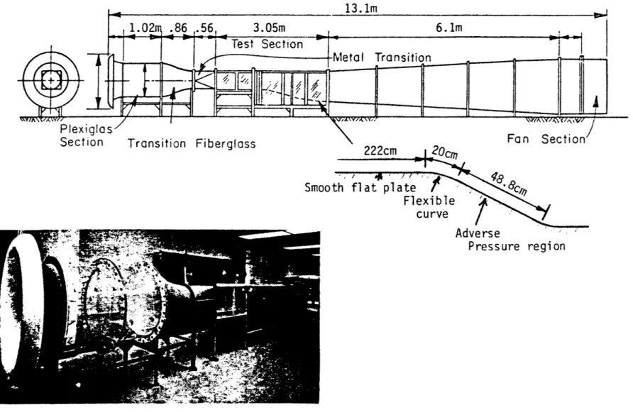
The experiments were made in a small, 45.7 x 45.7 cm, open return wind tunnel, figure 1. The test section consisted of a near zero pressure gradient region of 190 cm in length. The turbulent boundary layer was approximately 6.4 cm in thickness, and a momentum thickness Reynolds number of4050 was developed at the measuring station for a freestream velocity of 10.2 m/sec. The static pressure distribution along the centerline of the test surface is shown in figure 2. For the zero pressure gradient studies a surface-hot-wire was located at x

= 198 cm. A detailed evaluation of the flow at this

loca-tion is given by Chien and Sandborn (1981). For the adverse pressure study a surface-hot-wire located at x

= 250 cm was used to indicate changes in the

surface shear. Since the present study was of an exploratory nature, most of the tests were made at a freestream velocity of 10.2 m/sec. Only for one set of fins was the effect of Reynolds number explored.

Surface Shear Measurements.- The surface shear was evaluated from surface heat transfer measurements made with hot wires mounted directly on the surface, Sandborn (1981). P1atinum-8%tungsten alloy wire, .001 cm in diameter and approximately 0.13 ern long were mounted directly between copper conductors imbedded in a plastic surface, figure 3. The wires are 1ayed directly on the surface, but are not physically attached except at their ends. The use of buried wires are not desirable, since their frequency response to the surface fluctuations is limited. Film gauges were not used, since their effective length in the flow direction is large. The hot wire sensors were built on the special insert plugs, shown on figure 3. The plastic polymide surface was employed to reduce the heat transfer into the substrate. The plastic material was also black in color, which greatly facilitates the mounting of

the surface wires.

The transfer function between the measured surface heat transfer and the surface shear was obtained from evaluation of the boundary layer velocity profiles measured at the location of the sensor. A number of emprical rela-tions exist for surface shear or skin friction coefficient as a function of the velocity profile-momentum thickness Reynolds number for zero pressure

3

gradient turbulent boundary layers. Figure 4 is a plot of the local skin friction coefficient, cf' as a function of momentum thickness Reynolds number. Relations for cf, reported by Granville (1975), Prandtl (1927), and Bell (1979) are also plotted on figure 4. A second relation obtained by Bell (1927), which includes a second velocity profile parameter, form factor H, is also shown on fi gure 4. Typi ca 1 measured va 1 ues of ~ and H measured in the present study are plotted on the two parameter relation given by Bell. Between the different cf relations shown there is roughly a :3% variation in the values of cf. At the present time it is doubtful that the accuracy of cf can be obtained to better than !3% for the low velocity flows considered.

The large fluctuations of surface shear encountered in the zero pressure gradient turbulent boundary layer, produce a non-linear error in thecalibra-tion between the surface-heat transfer and-shear. A special technique outlined by Sandborn (1979) was used to correct the calibration for the

non-linear averaging. In order to reduce the calculation time an approximate relation was used to evaluate the surface shear for the measurements behind the different devices. The transfer function between the mean surface shear,

~w' and the output voltage of the hot wire (operating in a constant tempera-ture anemometer circuit) is assumed to be of the form, Sandborn U972)

(1) where E is the hot wire mean voltage output and e is the time dependent

voltage perturbation about the mean value. Taking th~mean of th~left ~

hand side of equation (1) results in terms containing e2, e3.

e4,

e5 and eO. It is assumed that all of the higher moments o~the perturbation voltage appear in terms that are small compared to the

e2

terms. Thus,equation (1) is approximated as

~w e AE2(A2E4 + 3ABE2 + 3B2) + 3Ae2(2A2E4 + 4ABE2 + 82)+8 3

(2)

For each measured value of E and e2 a value of ~ was computed. The values of A and B were determined from the corrected transfer function. The approxi-mation appears to give values of ~ within ±5% of values obtained by the more complex evaluation reported by Sandborn (1979). Repeat calibrations of the surface hot wire transfer function were found to vary by approximately ±4%, so the use of equation (2) does not appear to produce a measurable

error. The fact that the hot wire is not extremely sensitive to surface shear (i.e. ~w~ E6) helps to reduce the non-linear effects. The measure-ments are presented as a ratio to the undisturbed shear, which was obtained independently from velocity profile measurements. For each ratio the hot wi re measurement wi th and wi thout the shear modi fi cat; on devi ce in place was used. Thus, it was possible to correct for slight variations in the sensor

4

sensitivity due to small changes in flow temperature. Some uncertainty may exist in the measurements, due to the presence of local pressure gradients induced by the flow modification devices.

The ratio of the fluctuations with and without the modification devices was computed assuming a local linearization of the transfer function, Sandborn (1972). Since the surface hot wire is not highly sensitive to the surface shear, the error due to local linearization

(replacing the transfer function by its local slope) is quite small (see the evaluation of hot wire anemometer errors given by Sandborn (1972)). The main error in evaluating the fluctuations is associated with the accuracy of the transfer function. Individual evaluations of the fluctu-ating surface shear are uncertain by approximately ~%, although the accuracy of the ratios should not have nearly as high an uncertainty. For the present exploratory study both the mean and fluctuating voltages were measured with long time averaging analog volt meters.

Flow Modification Devices. - A number of devices have been tested as possible ways of increasing or decreasing the mean and fluctuating surface shear. A large number of different size fin sets were tested to determine possible trends toward an optimum geometry. Thin ribbons or plates placed parallel to the surface were employed in the basic study of the fluctuating surface shear. The results for thin plates near the surface are given in the companion report, Chein and Sandborn (1981). Some information on larger, thin plates, placed in the outer region of the boundary layer was obtained in the present study. Cylinderical rods placed both on the surface and at slight distances above the surface was included in the study. A thin airfoil with trailing edge blowing was also evaluated. Flexable strips, and solid and open fences were evaluated as possible devices for increasing the surface fluctuations. A number of different sizes and shapes of vortex generators were also evaluated. Sizes and construction details for the devices are given in Table I.

RESULTS AND DISCUSSION

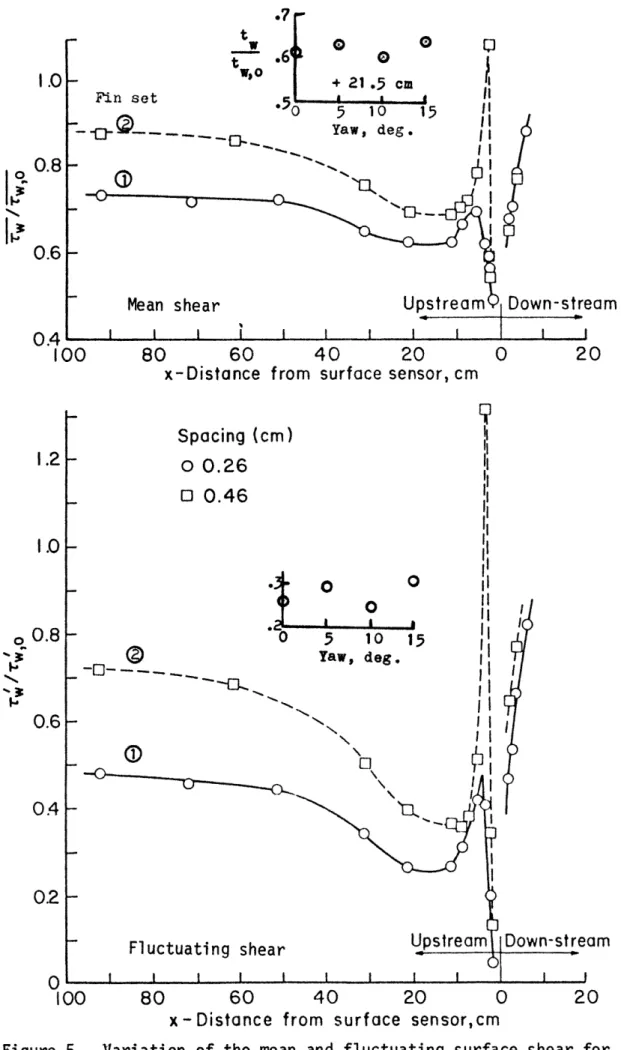
Zero Pressure Gradient Flow.-(FINS) Of the many devices tested the sets of closely spaced fins and the flexable elements were the most effective in reducing both the mean and fluctuating surface shear for the zero pressure gradient flow. Figure 5 shows typical variations of the mean and fluctuating surface shear ratios obtained by placing the sets of fins at various distances upstream of the surface hot wire sensor. The closely spaced (S

=

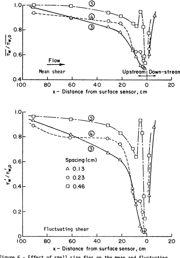
0.26cm) set of fins produce nearly a 30% reduction in the mean surface shearanda50%in't' reduction at a distance of 90cm upstream of the sensor. This upstream distan~e is equivalent to 14.6 boundary layer thicknesses of the undisturbed flow

at the hot wire location. Figure 6 shows measurements for a series of small sized fins. The smaller fins produce a pronounced effect at short distances upstream, but there reduction in the surface shear does not persist for as

5

The velocity distributions at the measuring station with the S =0.26cm spaced fins (figure 1) set at 20cm and 90cm are shown on figure 7. The fins produce a large momentum defect in the boundary layer near the surface. Smoke visualization directly down stream of the fins did not indicate a region of separation, although the very large drop in mean shear directly behind the fins would suggest a near separating condition. Directly behind the fins the surface shear fluctuations are nearly non-existant. The values of the fluctuating shear plotted near x = 0 are questionable, as they are approaching the noise level of the anemometer system.

As noted on the insert of figure 5, the alignment of the fins with the mean flow was not critical. A variation of 15 degrees from the mean flow direction produced practically no change in the mean shear value The insensitivity to slight flow angles should be of great value. It was de~on­

strated by Chien and Sandborn (1981) that the misalignment of the thin plates had a major effect on the surface shear.

Figure 8 is a review of the information obtained to date on the effect of fin-spacing, width and span. For the present boundary layer, fin spacings of the order of O.lcm would appear to produce the maximum reduction in both the mean and fluctuating surface shear. For direct drag reduction applications there may be a trade off between the spacing and the form drag of the fins. The width of the fin has not been evaluated sufficiently to make a definite statement on the optimum. Likewise the height of the fins need to be investi-gated further. The present study has also been limited to finite span of the fin sets. Figure 8c) suggests that the results are not critical for spans equal to or greater than the boundary layer thickness.

The effect of Reynolds number was investigated for the 0.26cm spacing fin set (figure 5). Figure 9 shows the measurements for Re = 4050, whqch were also plotted on figure 5, compared with measurements at Re = 3080. The percentage reduction in the mean shear is not as great for the lower Reynolds number flow as for the higher Reynolds number flow. The reduction in the fluctuating shear is approximately the same for both Reynolds numbers.

Zero pressure gradient flow. - (Other devices) A number of devices were investigated, which produced a momentum loss and reduction in both the mean and fluctuating surface shear. As noted previously, the use of thin plates, or ribbons near the surface was investigated in detail and the results are contained in the companion report Chien and Sandborn (1981). A number of other possible thin plate configurations, such as two plates in tandem were also investigated. The different thin plate configurations and the indicated shear are tabulated in Table II. In general the two plates in tandem produce a larger local reduction in the surface shear than a single plate, however. the effect persists for a very short distance downstream. As noted in the report by Chien and Sandborn (1981), the plates block the large fluctuation in surface shear from reaching the surface, but they do not alter the production of the large pulses.

6

In a private communication with the research group at Illinois Institute of Technology it was pointed out that they were modifying the large scale structure of the boundary layer by the use of thin plates placed in the outer region of the layer. Based on the limited information obtained, a series of single and tandem, thin plates were tested in the outer part of the boundary layer. The results of these tests are also included in Table II. While a reduction in surface shear was noted for the outer region plates,

the reduction was much less than that observed for either the plates near the surface or many of the other inner layer devices.

Figure 10 is a summary of tests made with a number of different devices: solid fence, open fence, flexable elements, rods on the surface, rods above the surface, jet blowing airfoil, sublayer vortex generators and a large scale vortex generator. Most of the devices show similar characteristics of a large increase in the mean or fluctuating surface shear directly down-stream. In one or two boundary layer thicknesses downstream the mean and fluctuating surface shear drops off to values usually less than the base flow value. By four or five boundary thicknesses, the effect of the device on the surface shear is usually quite small. The most surprising result

was that the large fluctuation generators, such as the rods above the surface, actually reduce the surface shear fluctuatien once they are one boundary

layer thickness upstream. It became evident that generation of fluctuations in the sublayer will not persist for any great length downstream.

The flexible element device (figure lOa) was a series of thin plastic strips glued to the surface and bent so they were vertical for no flow. The strips were 2.6am high (.4 of boundary layer thickness) and between .1 and .2 wide. They were free to bend backward in the flow. The device was not investigated until late in the study, so only a limited amount of data was obtained. Originally it was assumed that the flexable strips would act as turbulence generators rather than dampers. Obviously the strips are acting more as a compliant surface. The flexable elements should be further investi-gated as a means of reducing the surface shear.

The small vortex generators, shown on figure IOe), were able to increase the surface shear over short distances only. The devices were designed to produce the high and low velocity jets similar to the sweep-burst phenomenon observed in natural boundary layers. It was thought that the high velocity jets would produce a low pressure, which in turn would pull flow from the outer region of the layer inward. Unfortunately, the effect is not able to generate sufficiently large mixing to persist for more than a few boundary layer thicknesses. It may be worthwhile to investigate the small vortex generators further, and also to consider then in conjunction with the large scale generator.

It was found that the large scale vortex generator had no effect on the local surface shear until it was at least six boundary layer thicknesses up-stream.

7

Adverse pressure gradients. - The pressure gradient for the test surface is shown in figure

2.

The adverse pressure gradient region was proceeded by a strong favorable pressure gradient. Details of the velocity distribution in the adverse pressure region are given in Appendix A. An intermittent separation was indicated at x

=

266cm and a zero-surface-shear stress occurred at about x

=

273cm. In order to evaluate the effect of vortex generators on the surface shear near separation, a surface hot wire sensor at x

=

250cm was employed. Figure 11 shows the indicated change in surface shear produced by a number of vortex generators and deflector plates. The large scale vortex generator mounted far upstream in the zero pressure gradient region produced the largest effect

(8%)

on the mean surface shear. The large scale vortex generator also increased the surface shear fluctuations by 20 to 36 percent. The small scale vortex generators were unable to increase the surface shear by more than 1 or 2 percent, and they actually decreased the fluctuations. Defector plates set parallel to the ramp gave roughly the same magnitude of effect as the large vortex generator.

The particular flow studied is perhaps too severe in both the favorable and adverse pressure gradient regions. A flow with milder conditions might be a better test of devices for the delay of separation.

CONCLUDING REMARKS

The present study demonstrates the value of the surface hot wire-shear gauge in evaluating the effect of modification devices. Devices, such as

rods, were thought to produce effects that last for long distances downstream. Measurements of the velocity profiles and turbulence would suggest that many boundary layer thicknesses are required for the flow to recover. The present measure of surface shear suggests that the disturbances do not persist at

the wall for more than a few lengths.

The major effects of the fins in reducing both the mean and fluctuating surface shear suggest that the lateral or 3-dimensional aspects of the turbu-lence is important. It was observed that thin ribbons or plates could block the fluctuation from reaching the surface, but in no way do the plates alter the development of the fluctuation downstream. Thus, the fluctuations would appear to be controlled by the lateral effects. At present it is not clear just how the fins (or the flexable elements) damp the large scale surface shear fluctuations.

It was assumed that the generation of fluctuations by a number of devices would pose no problem. However, it was not foreseen that

turbu-lence generated near the surface can not persist for long distances. Only the large scale disturbances developed by such devices as large vortex generators that extended across the total boundary layer thickness appear to be able to persist for the large distances required to delay boundary layer separation.

REFERENCES

Bell, G. J. (1979); Turbulent boundary layer skin friction predictions. Masters Thesis, Colo. St. Univ.

Chien, H. C., and Sandborn, V. A. (1981); A time dependent flow model for the inner region of a turbulent boundary layer. Colo. St. Univ. Report CER 80-81-HCC-VAS 45.

Granville, P. S. (1975); Drag and turbulent boundary layer of flat plates at low Reynolds numbers. David W. Taylor Naval Ship Research and Development Center Report 4682.

Prandtl, L. (1927); Uber den Reibungswiderstan Stromender Luft, Reports of the Aerod. Versuchsanst. Gottingen, 3rd. series.

Sandborn, V. A. (1972); Resistance Temperature Transducers. Metrology Press, Ft. Collins, Colo.

Sandborn, V. A. (1979a); Trends in turbulent boundary layer research. Proc. 3rd. Engr. Mech. Spec. Conf. ASCE, Austin, Tx.

Sandborn, V. A. (1979b); Evaluation of the time dependent surface shear stress in turbulent flows. ASME paper 79-WA/FE-17.

Sandborn, V. A., and Kline, S. J. (1961); Flow models in boundary layer stall inception. J. Basic Engr., Trans. ASME, ser D., vol 83, p 317.

FINS 1 w I J I ~ J I •

TABLE I. FLOW CONTROL DEVICES

vI;'

I/V

0.014 cm thick alwninul::1 sheet used for conntruction. Each fin 1.s !lade with

Height

V-I;'~-f'~

~~ ~

a 90 deeree bend at bottom of the width of the spacing. Each fin is glued to a

0.014 cm thick sheet. The sheet is in turn glued to the vdnd tunnel surface.

\

J

u

,

,. . _77~ Spacing / ' Width ID width hei0ht C:c.l em 1 .3.22 1.75 2 3.t8 1 .79 .3 .3 .190 .765 4 2.591 .795 5 2.596 .780 6 .3 .13 .765 7 2.6 .767 () _{.635t03 .18.791} 9 2.54 20DS Diameter Cf:l .122 .173 .320 }'EHCES .79 JlenGth cm 33.3 33.3 .5.3.3 Open

t

.64 em ~ spacing span cm crn .264 15.09 .462 21 .07 .13 11 .71 .23 19.49 .462 21 .07 .13 2.35 to 11 .7 .45 .168 3.05 .102 2.54 Remarks

on surface and 2 C1-:1 above

on surface only

on surface and 0.36 cm above

I

~

I

I"

III?

.066 en diameter rods

:', Jl

n "

~:{ ~1

T_A<

O. 11 em high and 0 .13 em

, > ; , > ; > ; , >; > > ; ; > ; wide

Flow I~ 0.014 cm aluminum

_ _ _ _ _ _ _ _ _ _ • > ; j ; >(;O;~: em high and 12.6 em span

Solid FLEXABl.E E~E!{8HTS

t

2.6cm

~

... 11 cm ~ 15 cm \Vide 01 cm thick plastic

II

III

"II

\1.

.

III

'11 _'I ~. ,I I' 1111 "I' \Ii 1/\ ~; ,,\ _III

I II· .014 cm aluminum plate

BLOWING AIRFOIL

I-

1 .63em

- - I

.1 90cm.I ( : ~ .076cm slot

TABLE I. (Cone2.uded) li'LO\![ CONTROL DEVICES VOL~TEX GElf.c!RATORS 1. Large seale 4 em high 2. Small scale

1~5

( f6()

(1 ()

(lhngle

1.8

em high "1/ em spacing 3. Small scale 1.8 em high 4. Large scale

\ /, \ / \/ \ / \ / 1:.5 5.3

em high 1 .5 .5 all dimensions in em

1. 5.1 em \vide, 5 Loeation* em 3.6 13.6 23.6

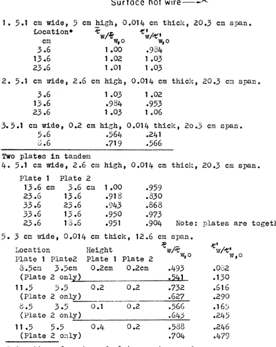
TABLE II. THIN PLATE TESTS

em high, 0.014 em thick, 20.3 em span.

:t- ~I w/i w/-'t't w,o w,o 1 .00 .984 1 .02 1 .03 1 .01 1 .03

2. 5.1 em \vide, 2.6 em high, 0.014 em thick, 20.3 C!11 span.

3.6 13.6 23.6 1 .03 .984 1 .03 1 .02 .953 1 .06

3.5.1 em wide, 0.2 em hieh, 0.014 thick, 20.3 em span. 5.6 .564 .241

J.6 .719 .566 Two plates in tandem

4. 5.1 em \vide, 2.6 em high, 0.014 cm thick, 20.3 em span. Plate 1 Plate 2 13.6 em 3.6 em 1.00 .959 23.6 13.6 .918 .830 33.6 23.6 .943 .868 33.6 13.6 .950 .973 23.6 13.6 .951 .904 Note: 5. 3 em wide, 0.014 em thick, 12.6 em span.

~ 1.-Location Height W/~ PIa te 1 PIa te2 Pia te 1 Plate 2 w,o

8.5co 3.5cm O.2em 0.2em .493 (Plate 2 only) .541 11.5 5.5 0.2 0.2 .732 (PIa te 2 only) ______ .627 d.5 3.5 0.1 0.2 .566 (Plate 2 only) .64j 11.5 5.5 0.4 0.2 .588 (Plate 2 only) .704 plates are ott VI/'tl W,O .082 .130 .616 .290 .165 .245 .246 .479

* Location of center of plates upstream of sensor.

TABLE II. (Concluded) THIN' PI .. ATE TESTS 6. 0.014 cm thick, 12.6 cm span

~ _~~/~.

Location Height Width Vl~

Plate 1 Plate 2 Plate 1 Plate 2 Plate 1 Plate 2 w,o w,o 7.75cm. 3.5c111 O.2cm 0.2cm 1.5cm 3cm .557 .138

(Plate 2 only) .621 .218

8.5 2.75 0.2 0.2 3.0 1 .5 .590 .246

(Plate 2 only) .706 .358

Two plates directly above each other

7. 3 cm wide, 0.014 cm thick, 12.6 em span, plate 1 - 0.4 em high.

Location _~w/t ~, _{plate 2 - 0.2 em high}

el!l w,o \'l/~\~,o -.5.5 .843 .779 -4 .792 .711 -1 .5 1.04 .465 +3.5 .583 .164 5.5 .616 .247 8.5 .734 .503 11 .5 .781 .563 21.5 .868 .739

Three plates directly above eaeh other

,

3 em wide, 0.014 cm thick, 12.6 cm span, plate 1 - 0.8 cm high

~.)

.

3.5 .545 .216 plate 2 - 0.4 cm high 21 .5 .815 .689 plate 3 - 0.2 cm high

13.1m _~ .86 ,.56 3.05m 6.1m Test Section .f- I ~1etal Transition

J

, ,\\'(;'/

)

Fan Section Transition Fiberglass 222cm

Smooth'

1:,

at· p', ;te '"

Flexible curve '18 , . 8_e . . ;-0... -...:. ' "

J

Adverse ' ; Pressure reg; on

...

.

4-f (I) o t.) s::: .~ 3.0 ...., o .,..,

t!

Flow 0.23 cm brass tube Polymide insert 0.001 cm Diam. Pt-8%Vl wire , I ,'!J , j

Figure 3. Surface hot wire-heat transfer sensor.

2 3 4

Bell, one parameter Bell, two parameter Granville

Prandtl

5 6xlcY

I·tomentum thickness Reynolds No. Figure 4.- Local shear stress determination.

1.0 Fin set t ...!. t _.,0

--o-~---_r"l

LJ""' _ _ + 21 .5 em .50~--!~~-~ Yaw, deg. ...

-I

~ 0.8

.!"

... ...

I~

0.6 Mean shear OA---~--~--~--~~~~--~--~--~--~~ 100 80 60 40 20 0 20

x - Distance from surface sensor, cm

~ Spacing (cm)

~

1.2 _00.26 ,I ,I

o

0.46

I'

,I

" 1.0 ,I " 0 _" 0 II 0 II _II

·1

I I , II ~ 0.8 • 0 5 10 15 @ 'I .... ~ _{Yaw, deg •} .... -0'-" -- -- ... ___ _{' I I} ... _---0... " .... ~ _... ... : I .... ... "-0.6

_"

, I '-

,

, I (.1)

_"

_~:

0 --().. _\ '""0

_"

,

I I l 0.4

_'U.

...

-02 Fluctuating shear O---~---~--~--~----~--~--~ 100 80 60 40 20

o

20

x - Distance from surface sensor t em

figure 5.- Variation of the mean and fluctuating surface shear for two sets of fins.

I

~ ~ "-1.0 0.8

1~0.6

Flow

..

Mean shear Upstream Down-s tream

0.4~----~---~---~----~---~---o

...

_...

"-...

100 1.0 0.8 0.6 ... 0.4 0.2 80 60 40 20

o

x - Distance from surface sensor, cm

-0-- - - -

--o-- ___

G>

'a.,

---~

R

... _

®

"'tJ...

/9

---0-

---0.."

'\,

I

I

G>

'Q,\,

\i \

1

Spacing (em)

?

\ I " 6 0.1:3 \ \

I"

,

o

0.23 • : o 0.46 Fluctuating shear

I :

o

, I

_,

_.

~ '0 \ \ 20 o---~---~----~---~----~---~ 100 80 60 40 20

o

x - Distance from surface sensor 1 cm

Figure 6.- Effect of small size fins on the mean and fluctuating surface shear.

c

~ 0 base +20em +90em 6 em 6.35 6.86 7.37 6* em .991 1 .47 1 .61 !. e em .718" .813 1 .02 U H 2 1 .38 1 .81 1 .58 e _~wN/m .171 .107 .125 Re 4050 4530 5670 OL---~~---~---~---~---~ _{. 2 . 4 • 1 .0}

Figure 7.- Variation of the mean velocity distribution downstream of fi n set number

<D .

-t _w

r

_{wp .6} Mean shear a) Effect of spacing. Width ot tin, em b) Effect of width. 1 .0 .8 ~ w

r

_.,0

.6 Span ot tins, em c) Effect of span. 1 .0 tin sets .8

.-e'

.6 --!. ~.

·,°.4

~t --.:! ~,

.,0

.2 o o Fluctuating shear .2 .4 Fin spacing, em ,~

"U...J' "

, ... 'IJ, I "'0...

,

...

Width ot tin, em 10 20 Span ot tins, em

;e w

r

·t

o ~. --!.

-e'

_-to Reynolds number Mean shear 100

Distance from surface sensor, cm

•

....

--~

---Fluctuating shear

~oo

Distance from surface sensor, cm

2.0r-- lOT

't. ....-tt.,o C Solid fence 0

o

Open fence

<>

Flexable element Mean shear

Distance from surface sensor, em

a) Fences and flexable element.

o

0.32 em d1am.

fi-e 0.17 cm d1am. :' : ~ 0.12 em d1am.

.

,A.

,.

~

4.:-/:5:1 \

_,

Distance from surface sensor, em

b) Rods on the surface.

't' --!. IC'

",0

~,

..

3 2

I

1 2 ~

_.,0

1 °30 Fluctuating shear

Distance from surface sensor, em

A

I' \

~. \

Distance from surface sensor, em

;e.

r

_.,0

1.6 -00.32 cm diam. ~ 0.12 cm diam. 1 .0 ~t --!. ~, _{w,o •} T~ _ _ _ _ ~J

Mean shear Fluctuating shear

Distance from surface sensor, cm Distance from surface sensor, cm c) Rods above the surface.

4 3 i .

r2

_.,0

1 [] 2 mm h1gh

o

4 mm high Solid point DO blowing

ij

'.

I I , I , I

,

,

I ' I '

,

~

,

,

;J\

_..

4 3-t"' -!. ~t

.,0

2 1

R

"

I' _{I ,} I I I I I I • I I : I I

,

~ I I

1

~

I ,

,

,

I I C I

~

_..

.

_.

• ,

o

Distance from surface sensor, cm d) Blowing jet.

\

•

Figure lO.-(continued) Effect of different flow modification devices on the mean and fluctuating surface shear.

-i.

---~..,o ott

...

;t'

.,0

o Large scale

2.0-:r\r\

Sensor ~ behind jet 1 .5 1.0 2.0 1 • 1 •

<>/\/\

Mean shear -0- __

-

...

_{... - - -0-}

0.---

... .

-I:J.. ...

-a-•• ... -b- ..

from surface sensor, em

Fluctuating shear

A,'

-

-/:... _{~~ ~~} ~

..

.,

...

./::,.,..

---20

Distance from surface sensor, em e} Vortex generators.

c

10

Figure lO.-(Concluded} Effect of different flow modification devices on the mean and fluctuating surface shear.

;&.

---~ \f,0 -t' -!: -t' 22.2. em

o

Largg scale 012.5 ~180 Small scale t>3 em plate, .8 em high

<>5

em plate, 2.5 em high ~5 em plate, 5.0 em high Mean shear

Distance along the test surface, em

~o ~ " _ - - -fi~·D-... -fi~·D-...- . . . -fi~·D-...,."..a _ . _ -c-- .... 0-- --- C .. .., • .,.'" -• 6 A ..-•-• A· -• -• - - -• . .. .. .. t> A

·i

6~0-...L--~-=---'-~~....I..---I~..J

Distance along the test surface, em

Figure 11.- Effect of vortex generators and deflection plates on the surface shear in adverse pressure gradients.

APPENDIX A

EVALUATION OF THE FLOW IN THE ADVERSE PRESSURE REGION

The wind tunnel test surface was constructed to produce a region of zero pressure gradient flow and then an expansion region of adverse pressure gradient flow sufficient to cause boundary layer separation. The actual set up of the test surface was shown in figure 1. Figure A-I shows the analog evaluation of the potential flow coordinates for the model as it was set up in the tunnel. Although the potential flow analysis suggested a mild effect of the pressure gradient, the actual measurements indicate a more severe variation in the pressure. Figure 2 shows the measured static~essure along the model for three freestream approach velocities.

The flow was found to accelerate in the region of the initial model curvature and then has a very sharp increase in pressure once the curvature was reached. The sharp change in pressure at the start of the curvature was not desired. However, since the work was done concurrently with the upstream, flat plate measurements, Chien and Sandborn (1981). no atte~pt

was made to re-adjust the model for fear of disturbing the upstream conditions. The static pressure and mean velocity fields in the region from s

=

247 cm to 276cm, where visual observations indicated separation was occurring, were determined from a pitot-and a disk type static-probe. Figures A-2 and A-3 show the measured static pressure and velocity variations at fixed heights above the surface. While flow visualization with dust indicated separation was occurring between s

=

260 and 26Scm, the surface static pres-sure still shows a definite increase. However, the static prespres-sure above the surface at 3cm indicates very little change.

As a first apprOXimation, the boundary layer velocity profiles along the potential coordinates have been evaluated. Figure A-4 shows the

com-puted velocity profiles. The static pressure profiles are shown in figure A-S. The variation of the velocity profile form factors and momentum thickness

Reynolds number are shown in figure A~6. '

Whether the potential coordinate or a coordinate normal to the surface was used had little effect on the parameters for the s

=

248 and 2S6cm

stations. However, the parameters in the separation region are more sensitive to which coordinate system is used. Figure A-7 shows the boundary layer para-meters compared with Sandborn-Kline (1961) separation correlations. The

pro-files at s

=

266cm are close to the "intermittent" separation case. The velocity profiles at s

=

273cm for u

=

11.00 and a.SSm/sec. fall close to the

zero~surface-shear-stress separation case. The estimate of the separation region from flow visualization is consistent with the intermittent separation correlations of Sandborn and Kline. The recently proposed separation criteron in terms of Hand Re' Sandborn (1979), is compared, figure A-8, with the

present data. The values of Hand R plotted on figure A-8 correspond to the points where the curves of figure A-7 cross the Sandborn-Kline correlation curve. While the agreement of the present data with the separation criterion shown on fig

A-8

arereasonable, further considerations of the proper coordi-nates for defi ni n9 the boundary 1 ayer profi 1 es are i ndi cated. The separa ti on criteron of Sandborn (1979), is unfortunately based on the two data points shown. These two data points are subject to uncertainties of the same order as the present data.

a-Distance, cm

-3

Height model,

s-distance, cm a) Approach velocity 11.0 m/sec.

Height above model, em 10.6 7.62 5.08 a.54 s-Distanee, em b) Approach velocity 3.55 m/see.

-- - --15.24 ---12.70

--==_15.2

270 Figure A-2. static pressure variation above the model surface.

Height above the model, cm 10.2 7.62. 5.0 2.54 -2----~~----~----~----~----~---L----~----~----~ 235 2.70 2.80 s-Distance, cm c) Approach velocity 6.30 ~/sec.

Figure A-2.. (concluded) Static pressure variation above the model surface.

10 Height above the

8 • (,) Clodel, cm 7.62 6.35 5.08 3.81 Q) ~6 s OL---~----~---~----~----~---~~~~~--~----~ ~5 2~ s-distance, cm a) Approach velocity 11.0 m/sec.

u

Q)

~ _s

Height above the model, cm 7.62 5.08 - - ... 3.81 2.54 1 .27 .508 ... ~~5----~~--J---~----~--~~----~--~~----~---2~80 s-ciistance, cm b) Approach velocity 8.55 m / sec.

1.27 .508

O~ ____ ~~ __ ~~ ____ ~~ ____ l ______ ~tl~ ____ - L _ _ _ _ _ _ 'LI_~ _ _ ~~t ____ ~I.

235 240 250 260 270 280

s-distance, em c) Approach velocity 6.30 m/sec.

1 • • 260.4 266.4 273.4 4 2 4 6 n-d1stance, cm n-distance, cm

a) Approamvelocity 11.0 m/s. b) Approach velocity 8.55 m/s.

16

n-distance, cm

c) APproach velocity 6.30 m/s.

Figure A-4. Velocity distributions along the potential flow coordinates.

60 2 4 6 8 10 12 14 n-ciistance, cm a) Approach vel. 11.0 m/s. N ~ _:z:

..

s:lt <l

_..

~ 6 ~ CD M CD ~4 ·M 't:S CD

a

2 to to CD n-distance, cm b) Approach vel. 8.55 m/s.

~

0

L---'--'----L---'-~I---I--...I.._--J

o

2 4 6 8 10 12 14 16 n-ci1stance, cm

c) Approach vel. 6.30 m/sec.

Figure A-5. static pressure profiles along the potential flow coordinate.

3.B

2.6 H 2.2

1.B

Approach velocity m/sec 011 .0 OB.55 l:l. 6.30 1 .4 .,",::-_-:-':::-=-_-L. _ _ ~_--1--_--'-_----.J 245 s-distance, cm a) Form factor. s-distance, cm b) Momentum thickness Reynolds number. Figure A-6. Boundary layer parameters.

.3

-H Approach velocity m/sec 2 011 .00 [J _8.55 ~ 6.30 1 ~----~---~---~----~---~----~ . 1 5 . 2 .3 .4 5~/&

Figure A-? Comparison of the velocity profile parameters \v.1th the Sandborn-Kline separation correlations.

Simpson, Strickland, Barr

35 _{Present results}

H

Sandborn, Liu

2 .5. I I _1__ I ! J...--I

o

10 20 30 40 50 60 ...

Momentum thickness Reynolds no. x 10-.)

Figure A-B. Comparison of the zero-surface-shear-stress separation criterion of Sandborn (1979) with the ~e~surements.