The impact of missing data imputation on HCC survival prediction: Exploring the combination of missing data imputation with data-level methods such as clustering and oversampling

IN

DEGREE PROJECT TEKNIK,

FIRST CYCLE, 15 CREDITS ,

STOCKHOLM SWEDEN 2018

The impact of missing data

imputation on HCC survival

prediction

Exploring the combination of missing data

imputation with data-level methods such as

clustering and oversampling

ABDUL JALIL, WALID

DALLA TORRE, KEVIN

KTH ROYAL INSTITUTE OF TECHNOLOGY

Abstract

The area of data imputation, which is the process of replacing missing data with substituted values, has been covered quite extensively in recent years. The literature on the practical impact of data imputation however, remains scarce. This thesis explores the impact of some of the state of the art data imputation methods on HCC survival prediction and classification in combination with data-level methods such as oversampling. More specifically, it explores imputation methods for mixed-type datasets and their impact on a particular HCC dataset. Previous research has shown that, the newer, more sophisticated imputation methods outperform simpler ones when evaluated with normalized root mean square error (NRMSE). Contrary to intuition however, the results of this study show that when combined with other data-level methods such as clustering and oversampling, the differences in imputation performance does not always impact classification in any

meaningful way. This might be explained by the noise that is introduced when generating synthetic data points in the oversampling process. The results also show that one of the more sophisticated imputation methods, namely MICE, is highly dependent on prior assumptions about the underlying distributions of the dataset. When those assumptions are incorrect, the imputation method performs poorly and has a considerable negative impact on classification.

Sammanfattning

Forskningen kring data imputation, processen där man ersätter saknade data med substituerade värden, har varit omfattande de senaste åren. Litteraturen om den praktiska inverkan som data imputation metoder har på klassificering är dock otillräcklig. Det här kandidatexamensarbetet utforskar den inverkan som de nyare imputation metoderna har på HCC överlevnads klassificering i kombination med andra data-nivå metoder så som översampling. Mer specifikt, så utforskar denna studie imputations metoder för heterogena dataset och deras inverkan på ett specifikt HCC dataset. Tidigare forskning har visat att de nyare, mer sofistikerade imputations metoderna presterar bättre än de mer enkla metoderna när de utvärderas med normalized root mean square error (NRMSE). I motsats till intuition, så visar resultaten i denna studie att när imputation kombineras med andra data-nivå metoder så som översampling och klustring, så påverkas inte klassificeringen alltid på ett meningsfullt sätt. Detta kan förklaras med att brus introduceras i datasetet när syntetiska punkter genereras i översampling processen. Resultaten visar också att en av de mer sofistikerade imputation

metoderna, nämligen MICE, är starkt beroende på tidigare antaganden som görs om de underliggande fördelningarna i datasetet. När dessa antaganden är inkorrekta så presterar imputations metoden dåligt och har en negativ inverkan på klassificering.

Table of contents

1

Introduction ... 5

1.1

Problem Statement ... 6

1.2

Scope and Objectives ... 7

2

Background ... 7

2.1

Data Imputation with single and multiple imputation... 7

2.2

Data-level methods ... 8

2.2.1

Mean/Mode Imputation ... 8

2.2.2

K-nearest neighbor (K-NN) imputation ... 8

2.2.3

Multiple Imputation by Chained Equations (MICE) ... 9

2.2.4

MissForest ... 10

2.2.5

Factorial Analysis of Mixed Data (FAMD) ... 11

2.2.6

Synthetic Minority Oversampling Technique (SMOTE)... 11

2.2.7

Cluster-based Synthetic Oversampling ... 12

2.3

Machine learning algorithms ... 12

2.3.1

Maximal Margin Classifiers, Soft Margins and Support Vector Machines ... 12

2.4

Related work ... 14

2.4.1

Previous comparative studies of imputation methods and their results ... 14

2.4.2

Impact of missing data imputation methods on classification ... 18

3

Methods ... 19

3.1

Data ... 19

3.2

Data Imputation ... 21

3.2.1

Multiple Imputation by Chained Equations (MICE) ... 21

3.2.2

K-NN imputation ... 21

3.2.3

missForest ... 21

3.2.4

Factorial Analysis for Mixed Data (FAMD) ... 21

3.2.5

Z-score Transformation ... 22

3.2.6

K-means, K-means++ and silhouette and cluster-based oversampling ... 22

3.3

Parameters for the Support Vector Machine ... 22

3.4

Evaluation Metrics and Statistical Testing ... 22

3.4.1

Accuracy ... 22

3.4.2

F-measure ... 23

3.4.3

Area Under the ROC Curve (AUC). ... 24

3.4.4

ANOVA and Tukey’s Honest Significance Test... 25

5

Conclusion ... 29

6

Discussion ... 29

6.1

Poor performance of MICE compared to the other imputation methods... 29

6.2

Random forest, FAMD and the theoretical maximum of the support vector

machine ... 29

6.3

Future research ... 30

References ... 31

1 Introduction

Due to recent advancements in computational power, data-driven statistical research combined with machine learning algorithms has become an attractive complement for clinical research (Kourou et al., 2015; Obermeyer and Emanuel, 2016). Among the most challenging tasks addressed in the medical community is survival prediction. Survival prediction is classification whereby you predict in a binary manner, whether or not the patient is alive or not after a certain time.(Burke HB. Goodman PH. et al., 1997; Cruz and Wishart, 2006).This consists of analyzing clinical data and drawing patterns and conclusions from these.

The aim of this study is to improve the cluster-based oversampling method proposed by Santos et al. (2015) by combining it with different data imputation methods. The study conducted by Santos et al. (2015) consists of a small heterogeneous dataset of 165 patients, almost all of whom have missing data. Only 7 patients have a full patient profile. The dataset contains 49 features and an imbalance ratio of 1.62. Santos et al. (2015) utilized unsupervised clustering and created synthetic samples based on minority clusters (Barua, Islam and Murase, 2011).with Synthetic Minority Over-sampling Technique (SMOTE). SMOTE is a popular method to oversample imbalanced datasets (Chawla et al., 2002). Section 2.2. will explain this method in more detail. Before Santos et al. (2015) could do this however, they had to impute the missing data. They did so with K-nearest neighbor imputation (K-NN) (Hastie, Tibshirani and Sherlock, 1999). An approach which can handle mixed-type data to estimate missing values based on similarity measures. Recent studies however, suggest that there are imputation methods that outperform k-NN imputation for a range of datasets, such as MissForest and Multiple Imputation by Chained Equations (MICE) (Stekhoven and Bühlmann, 2012a). Whether k-NN imputation was the right choice for Santos et al. (2015) deserves further study, since we consider this the weak part of their paper.

Small datasets with missing values are especially challenging because they limit the scope of data mining techniques since they may not provide enough information so that the learning task may be accomplished (Andonie, 2010). However, small datasets with a large number of features and correlations between features are common among medical data (Mazurowski et al., 2008). Missing data is unavoidable in clinical research and its potential to invalidate research results are often overlooked (Wood, White and Thompson, 2004). Inadequate handling of these missing data in the analysis may produce biased models and false results on classification, which therefore decreases their performance (Wood, White and Thompson, 2004; García-Laencina, Sancho-Gómez and Figueiras-Vidal, 2010a). The reasons for missing data in clinical trials are many, but a few examples include: Hospitals don’t always have all the equipment available, missed appointments and outright refusal to respond to personal questions (García-Laencina, Sancho-Gómez and Figueiras-Vidal, 2010b) Regarding missing data, Little et al.(1987) define the following situations: Data are “missing completely at random” (MCAR) if the probability of a missing outcome does not depend on any baseline covariates and is therefore the same for all individuals. Next is missing at random (MAR), which allows missingness to depend on any observed data. An example would be missing values that are determined by observed outcomes as a trial progresses. Finally, missing not at random (MNAR) is used to describe situations where the probability of a missing outcome depends

on unobserved outcomes as well as on observed data. An example of this would be a patient that leaves a study because of a detoriation. There are numerous ways of handling missing data, which includes removal or imputation (Taylor and Little, 2012). Imputation is the process of replacing the missing data with substituted values through various methods (van Buuren et al. 1999, 2011; Sterne et al. 2009). Different imputation methods will be central to this study and will be more thoroughly explained in later sections. Removing data with missing data will give too few data points in this case. Which is a bad idea since there are few data points to start with (Scheffer, 2002).

1.1 Problem Statement

Santos et al. (2015) did not combine their cluster-based oversampling with a range of different imputation methods since that was not their primary focus. While k-nearest neighbor imputation is not without its merits, a study by Stekhoven & Buhlmann (2012b) for example, indicated that MissForest outperformed k-NN as an imputation method for 11 different data sets which included continuous data, categorical data and mixed-type data at different rates of missingness. They then compared the different methods by looking at the NRMSE (Normalized Root Mean Square Error) values for continuous data and at the PFC (Proportion of Falsely Classified) values for categorical data. Our problem statement therefore is to test a variety of different imputation methods which we believe have merit, on the data used by Santos et al. (2015) so that we can then test whether or not their choice of imputation method can be improved. Since other imputation methods could possibly better capture potential underlying non-linear relations and complex interactions, they could potentially improve classification results (Stekhoven and Bühlmann, 2012b). Our focus will therefore be to test different imputation methods and combine their results with the cluster-based oversampling methodology proposed by Santos et al (2015). Together with a Support Vector Machine (SVM) classifier, we will look for changes in performance that are statistically significant. The tests are mentioned in sections 1.2. and 2.4.

Our hypothesis is drawn mainly out of two studies. The first one by Stekhoven et al (2012b) and the second by Audiger et al. (2016). As shown by the study of Stekhoven et al. (2012), MissForest outperformed k-NN and even MICE in almost all cases for a wide range of datasets. They compared NRMSE and PFC values. MissForest is able to better to impute datasets that contain complex interactions and non-linear relationships between variables. If the relationships between the variables in the HCC dataset are strongly non-linear, we expect MissForest to be a superior imputation method. The idea is that this will eventually be reflected in the final results of the survival prediction because the imputed data better reflects the true values that would have been there, had there not been any missing values. Provided that we balance the class weights prior to imputation. The second study, by Audiger et al. (2016) confirms this assumption when they compare MissForest to their own method, FAMD. FAMD is a more sophisticated method that also performs well for most datasets. But the study showed that it outperformed MissForest when the datasets contained variables with strong linear relationships, since it uses principal component methods.

MICE is a bit of toss-up. If our assumptions regarding the probability distributions of each variable are correct, then MICE should also give better results. It can be difficult to capture underlying distributions and Stekhoven et al. (2012) show that k-NN sometimes outperformed MICE and sometimes vice versa. Therefore our

expectation is that the cluster-based oversampling method in combination with either MissForest or FAMD will significantly change the results of an HCC survival prediction study such as the one carried out by Santos et al. (2015)

1.2 Scope and Objectives

There is no universal method for handling missing data in a clinical trial, since each trial is different in the way it is designed (Little et al., 2012). In this study we will apply & compare four different imputation methods on the same data set, i.e. the one used by Santos et al. (2015). Santos et al. (2015) constructed four different test cases on one single dataset. They trained their neural network classifiers in the following four approaches. First approach is to train the neural network classifier without clustering or oversampling. The second approach was to oversample using SMOTE, but without clustering. The third approach was what they call the representative set approach. The representative set approach means clustering the data using k-means. The clustering process is run multiple times (multiple initializations) giving multiple different partitions and then merging 20% of each into a large representative set M. The fourth and final approach only differs in the final merging process. In the last approach R different datasets are created by taking each of R partitions and combining them with R – 1 portions of the samples of the remaining data sets. Each of these R datasets are then used for training. Thus, producing R different models, and their resulting R predictions are combined using majority voting. This is what they call the augmented set approach.

The four methods that we want to try can each handle heterogeneous data, i.e. a mix of continuous, nominal and ordinal data whilst being very different from each other in the way they impute the data. This gives us an ability to consider data with different characteristics. The objective is then to follow the data-level methods proposed by Santos et al. (2015) by first using cluster-bused oversampling to balance the dataset then train a support vector machine (SVM) classifier and then finally, carrying out three common but different evaluation metrics, Accuracy, F-measure and AUC (Bradley, 1997; Powers, 2011), to evaluate mean and standard deviation. See Section 2.4. for a description for each of these.

2 Background

2.1 Data Imputation with single and multiple imputation

This study focuses on handling missing data through imputation rather than deletion. When small data sets contain missing data, deletion is often ruled out from the beginning (van Buuren, 2012). Instead, the focus is on imputation, which means substituting the missing values. Single imputation methods are methods that substitute

the missing values once and then treats them as if they were true data. That means they do not account for uncertainty in the models. Multiple imputation however, fills the values multiple times and thus give you multiple imputed datasets. Because they involve multiple predictions they can account for uncertainty in predictions and return accurate standard errors. If there is a lot of missing data, the different imputations will vary strongly and yield high standard errors. If the data is predictive with a low missing value ratio, then the predicted values will have a low variation and imputations will be consistent. This will lead to smaller but still correct standard errors (Azur et al., 2011; van Buuren and Groothuis-Oudshoorn, 2011).

2.2 Data-level methods

The data-level methods that are implemented in this study consists of five imputation methods (mean/mode imputation, k-nearest neighbor imputation (K-NNI), Factorial Analysis of Mixed Data (FAMD), Multiple Imputation by Chained Equations (MICE) and Imputation with Random Forest (MissForest)). It also consists of two other data-level methods: Synthetic Minority Oversampling Technique (SMOTE) and K-Means. The imputation methods were chosen either because they are the most common in the literature that we studied or because they show merit in performance (Stekhoven and Bühlmann, 2012b). They range from the simplest to more the sophisticated methods.

2.2.1 Mean/Mode Imputation

Mean and Mode imputation are more of a quick fix for imputation but might sometimes be satisfactory. When you have continuous data, you take the mean of all available values for the variable and use it as the imputed value. Mode can be used instead of the mean for categorical data. When using mean/mode imputation, at least you can make sure that the values do not exceed the minimum or maximum. However, mean/mode imputation will most likely distort the data or the underlying distribution and will bias any estimate other than the mean (van Buuren, 2012). Why use this method then? Other than it being a fast and easy method, mean/mode is often used as a starting point (initialization) for more sophisticated methods. In this study, Mean/Mode imputation will only be used as an initialization for the more sophisticated imputation methods.

2.2.2 K-nearest neighbor (K-NN) imputation

K-nearest neighbor (K-NN) imputation method is a non-parametric imputation method capable to handling both continuous and categorical data-types (Jerez et al., 2010). K-NN approximates the data locally. The method uses the k nearest examples in feature space to impute the data. If the missing value belongs to a continuous variable, then the missing value will be imputed with the mean of the k-nearest neighbors. If the missing value belongs to a class variable, then the value to be imputed will be decided by majority vote. Before the imputation begins, a distance metric must be defined. Heterogeneous Euclidian Overlap Metric (HEOM) is a metric that can be used for mixed data types. The distance metric d is defined as:

𝑑(𝑋_𝐴, 𝑋_𝐵) = √∑ 𝑑_𝑖(𝑋_𝐴𝑖, 𝑋_𝐵𝑖)2 𝑛 𝑖=1 (1) 𝑑_𝑗(𝑋_𝐴𝑗, 𝑋_𝐵𝑗) = { 1 𝑖𝑓 𝑥_𝑗 𝑖𝑠 𝑚𝑖𝑠𝑠𝑖𝑛𝑔 𝑖𝑛 𝑋_𝐴 𝑜𝑟 𝑋_𝐵 𝑑0(𝑋𝐴𝑗, 𝑋𝐵𝑗) 𝑖𝑓 𝑥𝑗 𝑖𝑠 𝑎 𝑑𝑒𝑠𝑐𝑟𝑒𝑡𝑒 𝑣𝑎𝑟𝑖𝑎𝑏𝑙𝑒 𝑑𝑛(𝑋𝐴𝑗, 𝑋𝐵𝑗) 𝑖𝑓 𝑥𝑗 𝑖𝑠 𝑎 𝑐𝑜𝑛𝑡𝑖𝑛𝑢𝑜𝑢𝑠 𝑣𝑎𝑟𝑖𝑎𝑏𝑙𝑒 } ₍₂₎ 𝑑₀(𝑋_𝐴𝑗 , 𝑋_𝐵𝑗) = { 0 𝑖𝑓 𝑥𝐴𝑗= 𝑥𝐵𝑗; 1, 𝑜𝑡ℎ𝑒𝑟𝑤𝑖𝑠𝑒; } (3) 𝑑_𝑛(𝑋_𝐴𝑗 , 𝑋_𝐵𝑗) = |𝑥𝐴𝑗− 𝑥𝐵𝑗| max(𝑥_𝑗 ) − min (𝑥_𝑗) (4)

2.2.3 Multiple Imputation by Chained Equations (MICE)

In Multiple Imputation by Chained Equations (MICE) or Fully Conditional Specification (FCS), a series of regression models are run, where each variable with missing data is modeled conditioned up other variables in the data. To be clearer, a multivariate imputation model is specified on a variable-by-variable basis by a set of conditional distributions (van Buuren and Groothuis-Oudshoorn, 2011). The MICE algorithm can handle mixed-type data such as binary, continuous and ordinal. The algorithm can be summed up in 5 steps (Azur et al., 2011). Step 1:

Initialize the imputation with a simple imputation method such as mean/mode imputation. The initial imputed values will act as “placeholder” values.

Step 2:

One variable, denoted “var” for example, will have its imputed values set back to missing.

Step 3:

The observed values for the variable “var” in Step 2 are then regressed on to other variables in the imputation model. Meaning “var” will be the dependent variable in a regression model. This regression model will essentially work in the same way as those outside of an imputation context.

Step 4:

The missing values for “var” are replaced with predictions from the regression model. The predictions are drawn from a distribution with a Markov Chain Monte Carlo method (MCMC). Finally, “var” is used as an independent variable in the regression model for other variables.

Steps 2-4 are repeated for each variable that has missing data. Iterating this process several times will yield an imputed dataset. With enough iterations, the coefficients in the regression model tend to become stable. Doing this m times will yield m different imputed datasets. 10 iterations with up to 40 imputed datasets tend to be enough for convergence (Graham et al., 2007). The imputed datasets are then analyzed and finally pooled together through mean or majority vote. Figure 1 shows a representation of the process with m = 3.

Figure 1. Multiple imputation by Chained Equations scheme.

2.2.4 MissForest

MissForest is a non-parametric imputation method for mixed-type data. It is an iterative imputation method based on training a random forest. This method is attractive because of its computational efficiency and ability to cope with high dimensional data (Stekhoven and Bühlmann, 2012b). Stekhoven & Buhlmann (2012) introduced this imputation method in order to create a method that could handle any time of input data yet makes as few assumptions as possible. According to studies by Stekhoven et al. (2012) the method is competitive to or outperforms many common imputation methods regardless of type composition, data dimensionality and amount of missing values. Datasets that contain complex interactions and non-linear relations are hard to capture with parametric procedures. Parametric procedures require tuning of a parameter. The choice of parameter without prior knowledge is difficult and could lead to a strong reduction in the methods performance. Since MissForest does not make any assumptions about the data, it could better capture these complex interactions and non-linear relations. Just like MICE, the algorithm uses mean/mode imputation to make an initial guess, after that, a random forest will be trained on the observed values and continue to predict missing values until some stopping criterion is reached. Since the method averages over many unpruned classification or regression trees, MissForest can be considered a multiple imputation method. Just like MICE. Using out-of-bag (OOB) error rates, imputation errors can be predicted without the need of a test set. Stekhoven et al. (2012) show that the difference between OOB error rates and real error rates usually do not differ more than 10-15%.

Finally, Random forests are built on decision trees, and decision trees are sensitive to class imbalance, therefore MissForest will be too. However, this can be mitigated somewhat by assigning class weights prior to imputation.

2.2.5 Factorial Analysis of Mixed Data (FAMD)

The final imputation method is called Imputation using Factorial Analysis of Mixed Data (FAMD) (Audigier, 2016b). It is a principal component method to impute missing values for mixed data. Since it is based on a principal component method, it studies the similarities between individuals and relations between variables. When you have a matrix of mixed-type data, you transform the categorical variables into dummy variables (called the indicator matrix) and concatenate them with the continuous variables. Then each continuous variable is centered and divided by its standard deviation (also called standardization). The dummy variables are divided by the square root of the proportion of individuals taking the associated category. The missing values are initially imputed using mean. Then principal component analysis (pca) is performed iteratively on the matrix, using Singular Value Decomposition (SVD) until a certain threshold is reached. Audiger et al. (2016) compare the FAMD imputation with that of MissForest (Stekhoven and Bühlmann, 2012b) for a range of datasets. They show that when there are strong linear relationships between the continuous variables, FAMD outperforms MissForest. In addition, when the percentage of missing values increases, the NRMSE of FAMD increases only slightly, whereas the NRMSE of MissForest increases more. Finally, when there are strong nonlinear relationships between variables, MissForest performs better but only slightly. Their study shows that FAMD remains a competitive imputation method in all cases.

Figure 2. FAMD method. Source: (Josse and Husson, 2016)

2.2.6 Synthetic Minority Oversampling Technique (SMOTE)

Another data-level method in this study is SMOTE (Chawla et al., 2002). Machine learning algorithms are usually designed to improve accuracy by reducing error (Chawla, Japkowicz and Drive, 2004). Most do not take into

account the class distribution. This can be dealt with by either oversampling or undersampling. Undersampling means removing the majority the class in order to balance the dataset. Oversampling refers to when you create more minority class points in order to balance the dataset. This can be done by randomly replicating minority classes, but this risks overfitting. SMOTE was proposed by Chawla et al. (2002) in order to oversample while reducing the risk of overfitting. SMOTE works in such a way that synthetic points are created by randomly choosing a minority sample, then choose one of its k nearest neighbors. After that, generate a number between 0 and 1 and multiply it with the difference between the nearest neighbor and the minority sample and add the total to the minority sample. This reduces the risks of overfitting since synthetic samples are created between the minority sample and its neighbors, not just replicated.

2.2.7 Cluster-based Synthetic Oversampling

Cluster-based Synthetic Oversampling is an oversampling method that utilizes SMOTE. The data is clustered using any clustering method, such k-Means (Kanungo et al., 2000) with an appropriate number of clusters. The appropriate number of clusters can be determined using methods such as the Gap statistic or the average silhouette method (Rousseeuw, 1987) . The average silhouette method computes the average silhouette of observations of different k-values. When considering a range of k values, the optimal number of clusters is the one that maximizes the average silhouette. The Gap statistic is another method for finding the optimal number of clusters. It tries to maximize the intra-cluster variation (Tibshirani, Walther and Hastie, 2001). However, clustering is not the primary focus of this study as such we refer to the references. Santos et al. (2015) used K = 10 in their study, assessing K values of a range of 2-30.

Once the samples have been clustered, oversampling is done within the minority clusters. That is the clusters with the lowest number of samples. SMOTE is then used but with a small difference. When over-sampling within the clusters with reduced sizes, the random number generated in SMOTE (0 to 1) is used to decide which class label the synthetically generated sample belongs to. If the value is below 0.5, the synthetic point is assigned a certain class label. If it is larger than 0.5, the sample is assigned the other class label. The assumption is of course, that there are only two classes in this case.

2.3 Machine learning algorithms

2.3.1 Maximal Margin Classifiers, Soft Margins and Support Vector Machines

A maximal margin classifier (Tibshirani et al. 2007) is a classifier that uses a hyperplane to separate classes in an input variable space. In two dimensions such a hyperplane would be a line. In three dimensions, the

hyperplane would be a flat surface. Using a linear equation that returns a scalar as an output to deal with a binary classification problem, any points that are above the hyperplane will be classified as belonging to one class, and any points that lie below the hyperplane will belong to the other. This can be decided by the sign of the output that the linear equation returns. This approach can be used to separate any points regardless of

dimensions. As long as the classes are linearly separable. In theory however, if the classes are linearly

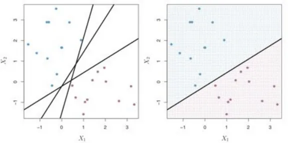
separable, then there are an infinite number of hyperplanes. Three such hyperplanes (lines) are shown on the left side of Figure 3. The natural way to choose the best hyperplane is to choose the hyperplane that is the farthest from the training observations. That is, to choose the hyperplane that has the largest perpendicular distance to the training observations on both sides. This is called the margin. The right-hand side of Figure 3 shows the line with the largest margin. The training observations that are closest to hyperplane are called support vectors because they decide where the hyperplane will lie. A single new observation may radically change the orientation of the hyperplane- Thus, it is better to use a soft margin. A soft margin means that we allow a few observations to be misclassified in order to make sure that the remainder of the observations are better classified. This will make the classifier robust to outliers.

Figure 3. Left-hand side shows possible seperating hyperplanes. Right-hand side shows the hyperplane with maximal margin. Source: (James et al., 2000)

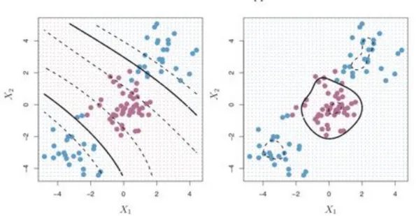
Finally, Support Vector Machines (SVMs) are a popular choice of classifiers that, according to Tibshirani et al. (2007), generalize the soft margin classifier. For cases that are non-linearly separable in a certain feature space, a method is needed to separate the classes. The SVM utilizes the kernel trick to map the original input space into a much higher-dimensional space, making the separation easier in that space. The kernel trick involves using the dot-product of vectors (points) using some kernel and then summing them up. Depending on which kernel is used, the decision boundary can be made non-linear. Figure 4 shows a decision boundary for a polynomial kernel (left-hand side) and for a Gaussian kernel (right-hand side) which is also called a radial basis

function.

Figure 4. Left-hand side: Decision boundary with a polynomial kernel. Right-hand side: Decision boundary. Source: (James et al., 2000)

2.4 Related work

2.4.1 Previous comparative studies of imputation methods and their results

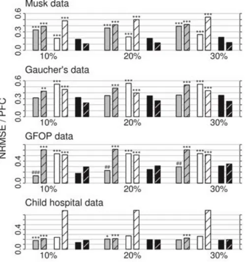
The literature on imputation of mixed-type data is rather scarce. In this section, we will present some key findings of two comparative studies involving imputation methods. The first one is a study by Stekhoven & Buhlmann (2012). As stated before, they introduce an imputation method based on Random Forest called missForest, in order to create a method that can handle any type of input data yet makes as few assumptions as possible. According Stekhoven et al. (2012) the method is competitive to or outperforms many common imputation methods regardless of type composition, data dimensionality and amount of missing values. Figure 5 shows the average NRMSE / PFC values for three different imputation methods: KNN, MICE and missForest using four different data sets with three different amounts of missingness. As can be seen on Figure 5, missForest (black bars) is either equivalent to or outperforms the other imputation methods.

Figure 5. Mixed-type data. Average NRMSE (left bar) and PFC (right bar), for KNN-Imputation (grey), MICE(white) and missForest(black). On four different datasets and three different amounts of missingness. Source: (Stekhoven and Bühlmann,

2012a)

The average runtime for each imputation method and dataset is presented in Table 1. As can be seen from Table 1, missForest is slower than K-NN imputation but considerably faster than MICE despite outperforming MICE on every dataset. This study carried out by Stekhoven et al. and these metrics are in fact what motivated us to attempt new imputation methods.

Table 1. Average runtimes (in seconds) for imputing the datasets analyzed by (Stekhoven and Bühlmann, 2012a)

Stekhoven et al. (2012b) conclude that missForest allows for missing value imputation on any kind of data. That it can handle both continuous and categorical data simultaneously and that it outperforms common imputation methods such as K-NN and MICE (Multiple Imputations by Chained Equations).

The second comparative study is one done by Audiger et al,(2013). They introduce a principal component method to impute missing values for mixed data. Section 2.2.4. describes the method (FAMD) more generally. What is important is that the method proposed by Audiger et al.(2013) is compared to missForest for datasets where there are linear relationships between variables and for datasets where there are non-linear

relationships among the variables. Figure 6 shows the NRMSE and PFC values for missForest and FAMD. As can be seen, the values (errors) are lower for FAMD than for missForest. Moreover, when the percentage of missing values increase, the error for the FAMD algorithm increases slightly, whereas the error for missForest increases more. Audiger et al.(2013) point out that these results are consistent for all datasets where the

relationships between variables are linear.

Figure 6.Distribution of the NRMSE (left) and of the PFC (right) when the relationships between variables are linear for different amounts of missing values (10, 20, 30 %). White boxplots correspond to the imputation error for the algorithm based on random forest (RF) and grey boxplots to the imputation error for iterative FAMD. Source: (Audigier, Husson and Josse, 2013)

When the datasets contain strong non-linear relationships or strong interactions between categorical variables however, missForest will clearly outperform the iterative FAMD algorithm. This can be seen from Figure 7. Audiger et al (2013), based on these results, conclude that FAMD is a superior imputation method for datasets with linear relationships amongst the variables. When there are strong interactions between categorical variables or non-linear relationships, then Random Forest (missForest) will perform better.

These two studies combined, one by Stekhoven et al. (2012b) and one by Audiger et al. (2013) form the basis for why testing imputation methods and their effects on classifiers such as SVMs is so important and

worthwhile.

Figure 7. Distribution of the NRMSE (left) and of the PFC (right) when there are interactions between variables. Results are given for different amounts of missing values (10, 20, 30 %). White boxplots correspond to the imputation error for the algorithm based on random forest (RF) and grey boxplots to the imputation error for iterative FAMD. Source: (Audigier, Husson and Josse, 2013)

2.4.2 Impact of missing data imputation methods on classification

Previous work on missing data has focused mostly on comparing different imputation methods and assessing them in terms of accuracy of the imputation, using metrics such as normalized root mean square error (NRMSE). Not many studies have been made in terms of assessing the impact of imputation methods in more practical terms. Souto et al (2015) conducted a study examining the discriminative/predictive power of

imputation methods on classification of gene expression. Souto et al (2015), conclude that despite the fact that there might be clear differences in imputation performances assessed using metrics such as NRMSE and PFC, such differences could become insignificant when they are evaluated in terms of how they affect classification. They conclude that imputation methods have a negligible effect on classification and clustering methods. Among them, they tested K-NN imputation, Bayesian Principal Component Analysis (bPCA), support vector regression (SVR) on a range of 12 gene expression microarray datasets. The study conducted by Souto et al (2015) is important as it highlights the fact that despite clear evidence that some imputation methods

3 Methods

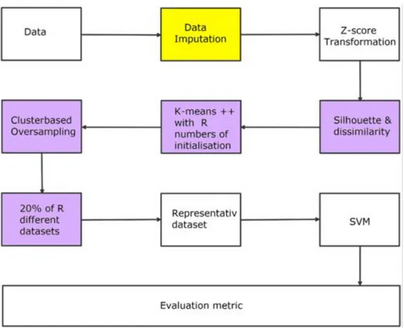
The methodology used in this study is depicted in Figure 8. Figure 8 shows a simple overview of the steps taken to reach the final results.

Figure 8. Depiction of the entire process. The steps colored in purple are stochastic processes and the yellow one indicates that different imputation methods where used.

3.1 Data

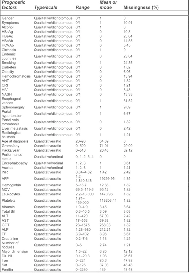
Before beginning any data analysis or pre-processing it is important to understand what type of data one has. The dataset, which was uploaded to the UCI Machine Learning Repository by Santos et al. (2015), was collected by Coimbra’s Hospital and University Center (CHUC). Since the original study by Santos et al. (2015) was a HCC survival prediction study, the dataset contains demographic, risk factor, laboratory and overall survival features from a set of N = 165 patients diagnosed with HCC. The dataset contains n = 49 features that were selected according to the EASL-EORTC (European Association for the Study of the Liver – European Organisation for Research and Treatment of Cancer) Clinical Practice Guidelines. A detailed description of the HCC dataset is presented in Table 2, which shows each feature’s type/scale, range, statistics (mean/mode) and missing rate percentage. It is important to note that this is a heterogeneous dataset, with twenty-three quantitative variables (all ratio scaled) and twenty-six qualitative variables. Overall, 10.22% of all data is missing, with only 7 out of the 165 patients having a full patient profile. The survival target variable is encoded as a binary variable with values 0 and 1. A value of 1 indicates that the patient survived after 1 year, and a value of 0 indicates that the patient died within that period. The dataset is imbalanced from the beginning with 102 cases as 1 (alive) and 63 cases as 0 (dead). The dataset was divided into a training set (85%) and a test set (15%)

Table 2. Characterization of CHUC’s hepatocellular carcinoma data. The dataset contains N = 165 records of n = 49 clinical variables, considered important to the clinicians decision process. The data was retrieved from Santos et al (Santos et al., 2015) but was originally collected by The Service of Internal Medicine of the Coimbra’s Hospital and Universitary Centre (CHUC)

Prognostic

factors Type/scale Range Mean or mode Missingness (%)

Gender Qualitative/dichotomous 0/1 1 0 Symptoms Qualitative/dichotomous 0/1 1 10.91 Alcohol Qualitative/dichotomous 0/1 1 0 HBsAg Qualitative/dichotomous 0/1 0 10.3 HBeAg Qualitative/dichotomous 0/1 0 23.64 HBcAb Qualitative/dichotomous 0/1 0 14.55 HCVAb Qualitative/dichotomous 0/1 0 5.45 Cirrhosis Qualitative/dichotomous 0/1 1 0 Endemic countries Qualitative/dichotomous 0/1 0 23.64 Smoking Qualitative/dichotomous 0/1 1 24.85 Diabetes Qualitative/dichotomous 0/1 0 1.82 Obesity Qualitative/dichotomous 0/1 0 6.06 Hemochromatosis Qualitative/dichotomous 0/1 0 13.94 AHT Qualitative/dichotomous 0/1 0 1.82 CRI Qualitative/dichotomous 0/1 0 1.21 HIV Qualitative/dichotomous 0/1 0 8.48 NASH Qualitative/dichotomous 0/1 0 13.33 Esophageal varices Qualitative/dichotomous 0/1 1 31.52 Splenomegaly Qualitative/dichotomous 0/1 1 9.09 Portal hypertension Qualitative/dichotomous 0/1 1 6.67 Portal vein thrombosis Qualitative/dichotomous 0/1 0 1.82

Liver metastasis Qualitative/dichotomous 0/1 0 2.42 Radiological

hallmark Qualitative/dichotomous 0/1 1 1.21

Age at diagnosis Quantitative/ratio 20–93 64.69 0

Grams/day Quantitative/ratio 0–500 71.01 29.09 Packs/year Quantitative/ratio 0–510 20.46 32.12 Performance status Qualitative/ordinal 0, 1, 2, 3, 4 0 0 Encephalopathy Qualitative/ordinal 1, 2, 3 1 0.61 Ascites Qualitative/ordinal 1, 2, 3 1 1.21 INR Quantitative/ratio 0.84–4.82 1.42 2.42 AFP Quantitative/ratio 1.2–_1,810,346 19299.95 4.85 Hemoglobin Quantitative/ratio 5–18.7 12.88 1.82 MCV Quantitative/ratio 69.5–119.6 95.12 1.82 Leukocytes Quantitative/ratio 2.2–13,000 1473.96 1.82 Platelets Quantitative/ratio 1.71–_459,000 113206.44 1.82 Albumin Quantitative/ratio 1.9–4.9 3.45 3.64

Total Bil Quantitative/ratio 0.3–40.5 3.09 3.03

ALT Quantitative/ratio 11–420 67.09 2.42 AST Quantitative/ratio 17–553 69.38 1.82 GGT Quantitative/ratio 23–1575 268.03 1.82 ALP Quantitative/ratio 1.28–980 212.21 1.82 TP Quantitative/ratio 3.9–102 8.96 6.67 Creatinine Quantitative/ratio 0.2–7.6 1.13 4.24 Number of nodules Quantitative/ratio 0–5 2.74 1.21

Major dimension Quantitative/ratio 1.5–22 6.85 12.12

Dir. bil Quantitative/ratio 0.1–29.3 1.93 26.67

Iron Quantitative/ratio 0–224 85.6 47.88

Sat Quantitative/ratio 0–126 37.03 48.48

3.2 Data Imputation

A total of four different imputation methods were used. For more information on how each method works, please see section 2.

3.2.1 Multiple Imputation by Chained Equations (MICE)

As stated in section 2.4.3. MICE is a method of sampling from regression models that have been specified for each variable. All binary variables were modelled using logistic regression, the ordinal data was modeled using an ordered logit model. The continuous data was modeled with either a normal distribution or with predictive mean matching. In order to find out whether a variable was normally distributed or not, a Q-Q plot was made in R. If the Q-Q plot is roughly in line with y = x, then normality was a reasonable assumption. If not, then predictive mean matching (PMM) was used. A total of 40 datasets were imputed with MICE. To be clearer, the HCC dataset was imputed 40 times, thus yielding 40 different “complete” datasets. Figure 9 shows to Q-Q plots, one of which is of a normally distributed variable and one of which normality cannot be assumed. The normally distributed variable in question is Mean Corpuscular Volume. The variable which is not normally distributed in Figure 8 is the Alanine transaminase.

Figure 9. Normal Q-Q plots. Left: Since the points lie roughly on the y = x line, normality is a reasonable assumption. Right: Normal distribution cannot be assumed.

3.2.2 K-NN imputation

For K-nearest neighbor imputation, HEOM was used as distance metric with k = 1. The reason for choosing K = 1 was mostly to replicate the same parameters that were used by Santos et al. (2015). Since K-NN imputation always returns the same values, this method only yielded one complete dataset.

3.2.3 missForest

MissForest is the name of the imputation method using Random Forest by Stekhoven et al(2012b). It was implemented in R using a prepared package by Stekhoven et al(2012b). The HCC dataset was imputed a total of 40 times using 100 trees per initialization, thus providing a total of 40 “completed” datasets.

3.2.4 Factorial Analysis for Mixed Data (FAMD)

Like the K-NN imputation, the iterative FAMD algorithm always returns the same imputed values. Therefore only one “complete” dataset was imputed using the missMDA package in R.

3.2.5 Z-score Transformation

As done by (Santos et al., 2015). Each column was transformed to have mean of 0 and a standard deviation of 1 using the Z-Score transformation. This was a necessary step for the later use of K-means. Since the only categorical variables in the HCC dataset are either binary or ordinal, there was no problem using a Z-Score transformation.

3.2.6 K-means, K-means++ and silhouette and cluster-based oversampling

The imputed datasets were clustered using K-means with K-means++ initialization. The number of clusters k was chosen to be k = 7. The number of clusters was based on the silhouette and the dissimilarity metric between clusters. The dissimilarity and silhouette were calculated for all k values between 2 and 30. A higher silhouette and a higher dissimilarity is considered good. Once the number of clusters was determined, a total of 20 K-means initializations were run. Each initialization gave different cluster sizes. In each initialization, the small clusters were oversampled with SMOTE to become the same size as the largest cluster. This was repeated until all of the clusters were the same size. Once that was done, 20% of the points in each initialization were chosen randomly and added up to a single large representative dataset. This was repeated for all the imputed datasets. For K-NN and FAMD, this process was repeated another 40 times, since they always returned the same imputed values. Depending on the sizes of the largest clusters, the representative datasets had somewhere between 1100-1400 data points.

3.3 Parameters for the Support Vector Machine

Once the representative datasets were created, a Support Vector Machine with an RBF kernel was trained in R using the Caret package. The parameter values that were tested and evaluated using a 50-fold cross validation were the values:

C: [0.1, 1.0, 1.5, 2.0, 2.5, 3.0, 4.0, 5.0, 6.0, 7.0, 8.0, 9.0, ...…, 128] : [0.001, 0.01, 0.1, 1.0]

These parameters were chosen on the basis of an initial run and provided the largest accuracy. Smaller values and larger values than the ones shown above only produced worse results. The number k = 50 in the k-fold cross validation was chosen to be as large as possible while making it computationally feasible.

3.4 Evaluation Metrics and Statistical Testing

Three different evaluation metrics were used. Accuracy, F-measure and AUC. Each metric had their mean and standard deviations evaluated. Each of them is described in the subsequent sections. Once all the necessary evaluation metrics were obtained, the results were analyzed using one-way ANOVA (Analysis of Variance) combined with Tukey’s honest significance test.

3.4.1 Accuracy

The confusion matrix in table 3 is commonly used in the evaluation of machine learning algorithms (Chawla et al., 2002). TN is the number of samples that actually are negative and has been classified as such. FN is the number of samples that are positive in reality but has been falsely classified as negative. TP is the number of

samples that actually are positive and has been classified as such. and FP is the number of negatives wrongly classified as positive

Table 3. Confusion Matrix. Predicted Negative Predicted positive Actual Negative TN FP Actual Positive FN TP

Accuracy is very common in the evaluation of performance in machine learning algorithms. It’s the proportion of correctly classified samples among all samples. This is a simple way of measuring the performance of models however its very sensitive to changes in the data. An example is given by Chawla et al. (2002) where the data is imbalanced. In the example the majority class accounts for 98% of the data so if the classifier always guesses the majority class it accuracy will be 98%. This is why accuracy is not appropriate when data is imbalanced however it will still be included to compare with the previous study. Accuracy is defined as:

𝐴𝑐𝑐𝑢𝑟𝑎𝑐𝑦 = 𝑇𝑃 + 𝑇𝑁

𝑇𝑃 + 𝐹𝑃 + 𝑇𝑁 + 𝐹𝑁

(5)

3.4.2 F-measure

F-measure consist of both precision and recall (Sasaki, 2007; Powers, 2011). The precision is the proportion of correctly classified positives among all samples classified as positive. Recall is the proportion of all real positive that are classified as such. Precision and recall are defined as:

Precision = TP TP + FP

Recall = TP TP + FN

(7)

The general definition of F-measure is:

𝐹_𝛽= (1 + 𝛽2_{) ⋅} 𝑝𝑟𝑒𝑐𝑖𝑠𝑖𝑜𝑛 ⋅ 𝑟𝑒𝑐𝑎𝑙𝑙

𝛽2_{⋅ 𝑝𝑟𝑒𝑐𝑖𝑠𝑖𝑜𝑛 + 𝑟𝑒𝑐𝑎𝑙𝑙}

(8)

The 𝛽 parameter adjust the influence ratio between precision and recall. The 𝐹1-measure is the special case 𝛽 =

1 and for this value of 𝛽 both will be equally important. 𝐹₁ is measure is defined as:

𝐹1= 2 ⋅

𝑝𝑟𝑒𝑐𝑖𝑠𝑖𝑜𝑛 ⋅ 𝑟𝑒𝑐𝑎𝑙𝑙 𝑝𝑟𝑒𝑐𝑖𝑠𝑖𝑜𝑛 + 𝑟𝑒𝑐𝑎𝑙𝑙

(9)

3.4.3 Area Under the ROC Curve (AUC).

Receiver operating characteristic curve (ROC curve) is a graph that has the true positive rate (TPR) on the vertical axis and the false positive rate (FPR) on the horizontal axis (Chawla et al., 2002; Powers, 2011). TPR is the proportion of correctly classified positives of all positives. TPR is the proportion of all negatives that are wrongly classified as positives. The ROC curve is a tradeoff between the true positive rate and the false positive rate wish are defined as:

TPR = TP TP + FN (10) FPR = FP FP + TN (11)

If the predictor is better than chance it should be above the diagonal and, the closer it is to the upper left corner (coordinate (0,1)) the better the predictor is. AUC is defined as:

𝐴𝑈𝐶 =𝑇𝑃𝑅 − 𝐹𝑃𝑅 + 1 2

Figure 10. ROC Curve

3.4.4 ANOVA and Tukey’s Honest Significance Test

ANOVA in its simplest form, provides a statistical test whether or not the means of several groups are equal. It generalizes the t-test to more than two groups. ANOVA was used in this study to test for statistical significance. It is used as an exploratory method. Tukey’s Honest Significance Test is used in conjunction with ANOVA as a post-hoc analysis. More specifically, it compares all the possible pairs of means and is based on a studentized range distribution. (Lisa Sullivan, Boston University)

4 Results

The first results obtained are shown in Figures 11 and 12. They show the intra-cluster

dissimilarity and silhouette for clusters ranging from K = 2 to K = 30. The figures clearly show

that K = 7 is a good choice and was thus our choice for the number of clusters.

Figure 11. The intra-cluster dissimilarity for clusters ranging from K = 2 to K = 30.

Figure 12. Silhouette for clusters ranging from K = 2 to K = 30.

After testing a range of parameters, we concluded that the value of C parameter in the SVM would be C = 8. This was based on the cross-validated accuracy. Figure 13 clearly show that the accuracy peaks around that range.

Figure 13. Accuracy (Cross-Validation) for different values of C ranging from C = 0.1 to C = 128.

The mean and the standard deviation were calculated for each of the three metrics, accuracy, F-measure using all four imputation methods. A quick glance at table 4 shows that the values for MICE are considerably lower than the rest.

Table 4: Mean and standard deviation of the different metrics and imputation methods.

Accuracy Accuracy F - measure F - measure AUC AUC

Mean std Mean std Mean std

KNN 0.735 0.05918246 0.8048035 0.04176155 0.696781 0.08221276 Random Forest 0.733 0.06034941 0.8023055 0.04705555 0.6953113 0.07489416 MICE 0.654 0.05696603 0.7455633 0.03988071 0.6024797 0.07799487 FAMD 0.72 0.0741447 0.7965862 0.05359123 0.6716888 0.09570455

One-way ANOVA was used to see if the results were significant. The H0 hypothesis is that there is no difference

between the imputation methods. One-way ANOVA test was done with a significance level of 𝛼 = 0.01 for accuracy, f-measure and AUC. The values are shown in Table 5,6 and 7.

Table 5: One-way ANOVA for accuracy.

Accuracy Df Sum Sq Mean Sq F value p

ind 3 0.1756 0.05852 14.73 1.7e-08

residuals 156 0.6196 0.00397

Table 6: One way ANOVA for F1-score.

F1-score Df Sum Sq Mean Sq F value p

ind 3 0.0944 0.031463 14.95 1.34e-08

Table 7: One way ANOVA for AUC.

AUC Df Sum Sq Mean Sq F value p

ind 3 0.2349 0.0783 11.34 9.01e-07

residuals 156 1.0768 0.0069

As shown in the tables 4,5 and 6 the chances of type 1 error are much smaller than the significance level for all of them. So the H0 hypothesis can be rejected with great certainty and Tukey's range test is the next step. The

P value is lower than the significance level 𝛼 = 0.01 for all rows when comparing MICE and FAMD. Tables 7,8 and 9 show the pair-wise comparisons in the post-hoc analysis (Tukey’s HSD).

Table 8: Tukey’s HSD for Post-Hoc Analysis for F1-score.

𝐅𝟏− 𝐬𝐜𝐨𝐫𝐞 Difference p Signif at p<0.01 ** ? MICE - KNN -0.059240121 0.0000002 Yes RandomForest - KNN -0.002497968 0.9949074 No FAMD - KNN -0.008217254 0.8538910 No

RandomForest - MICE .056742153 0.0000008 Yes

FAMD - MICE 0.051022867 0.0000102 Yes

Famd - RandomForest -0.005719286 0.9443918 No

Table 9: Tukey’s HSD for Post-Hoc Analysis for Accuracy.

Accuracy Difference p Signif at p<0.01 ** ? MICE - KNN -0.081 0.0000003 YES RandomForest - KNN -0.002 0.9989762 NO FAMD - KNN -0.015 0.7116476 NO

RandomForest - MICE 0.079 0.0000325 YES

FAMD - MICE 0.066 0.0000359 YES

Famd - RandomForest -0.013 0.7928599 NO

Table 10: Tukey’s HSD for Post-Hoc Analysis for AUC.

AUC Difference p Signif at p<0.01 ** ? MICE - KNN -0.09430125 0.0000064 YES RandomForest - KNN -0.00146975 0.9998217 NO FAMD - KNN -0.02509225 0.5322257 NO

RandomForest - MICE 0.09283150 0.0000092 YES

FAMD - MICE 0.06920900 0.0015378 YES

5 Conclusion

By looking at the results, we conclude that the choice of imputation method does have an impact of classification. It is clear from the statistical tests that the imputation method MICE performed worse than all the others. The reasons for this will be discussed in the next section. The differences between K-NN, Random Forest Imputation and FAMD were not statistically significant. This is somewhat surprising, as one of our hypothesis was that these methods would impute the data better and thus providing the support vector machine with a more representative dataset that better captured the underlying relations. Another research question was whether or not the choice of K-NN Imputation was a proper choice by Santos et al. (2015). The results show that on the HCC dataset, K-NN performed just as good as Random Forest (missForest) and FAMD. Therefore, we conclude that the imputation method chosen by Santos et al. (2015) was adequate and did not affect the classification in a negative way compared to the more sophisticated state of the art imputation methods mention above. Our study is limited however, and the conclusions drawn cannot be generalized. In order to study the impact of missing data imputation on classification in general, several more datasets need to be considered at different missing rates along with multiple classification methods. Section 6 will cover these limitations and propose further research for the future.

6 Discussion

6.1 Poor performance of MICE compared to the other imputation methods

As shown by Tables 8,9 and 10 Multiple Imputation by Chained Equations (MICE) performed significantly worse than the other imputation methods. MICE requires one to make assumptions about each features underlying distribution. Incorrect assumptions about these distributions could be one of the causes that make MICE perform worse than the other imputation methods. Another problem arises when the specified conditional distributions are incompatible. Recall that MICE repeatedly samples from conditional distributions: for example, with three variables X, Y, Z, it draws X from the conditional posterior [X | Y, Z], then Y from the conditional posterior [Y | X, Z], and so on. If we impute via a linear regression on one of the variables and impute another via ordered logistic regression, there is no joint distribution for the two variables which yields both these conditional distributions. Thus, this depends on the order of imputation and which variable was imputed last. According to Sterne et al (2009) however, whilst this may negatively affect the imputation, the mismatch between the assumed distribution and the true distribution has a larger negative impact on the imputation. Since we did not know much about the data, our assumptions about the underlying distributions could have been incorrect. The focus should be on the modelling issues instead.

According to the statistical tests carried out in section 3.4.4, the differences between the reminder of the imputation methods (missForest, FAMD and K-NN) were not statistically significant. Before discussing anything else, the issue of a theoretical maximum of the support vector machine (SVM) needs to be raised. If we instead had a hypothetical HCC dataset of similar size, but with no missing values, would the classification have been different? It is entirely possible that within the range of parameters tested, the SVM would have given us the same accuracy, F-measure and AUC values as those in Section 4. The fault then, does not lie with the imputation methods themselves but rather with the size and nature of the dataset and the limitations of the SVM to correctly classify the outcome. The SVM classifier would then have reached a theoretical maximum in which it could not be improved without additional data. Any small changes to this hypothetical dataset might not alter the decision boundary (separating hyperplane) of the SVM significantly. The HCC dataset provided by Santos et al. (2015) contains roughly 10% missing data, therefore the missingness rate itself is not high.

Next, one has to look at the stochastic processes in this study. Clustering the data using K-means and then oversampling the minority clusters with SMOTE introduces a lot of noise and variability. If the variations in the features of the synthetic data points are larger between each initialization of K-means and SMOTE than the variations in the values between each imputation method, then the clustering process will ultimately

overshadow the differences between the imputation methods. In the case of MICE, the mismatch between the assumed distribution and the true distribution could potentially be amplified by this oversampling process. Our hypothesis that MissForest imputation would impact classification in a positive way if the relations between the variables in the dataset were strongly non-linear, and vice versa for FAMD, turned out to be non-verifiable in this case.

In order to answer these questions more robust research needs to be carried done in the future. These proposals are presented in Section 6.3

6.3 Future research

Literature on imputation methods for mixed data is scarce, and literature on the impact of imputation on classification is even more so. In order to answer the question on how the missing data imputation methods used in this study impact classification, we propose that future research takes into account multiple

heterogeneous datasets of different dimensionalities. Each of these heterogeneous datasets should be complete and contain no missing data. We propose that researchers randomly remove data by introducing missing values completely at random (MCAR) and thus produce incomplete datasets at different rates of missingness such as 10%, 15%, 20% etc. This would make the research more robust by taking into

consideration different complexities of datasets. We then propose that classifiers are developed using support vector machines, neural networks and logistic regression models. This would help determine whether or not a theoretical maximum was reached as discussed in Section 6.2. By using multiple classifiers, the chances of a study being limited by such theoretical maximums are lowered. A large comprehensive study of this sort would be both helpful and informative for practical applications.

References

Andonie, R. (2010) ‘Extreme data mining: Inference from small datasets’, International Journal of Computers, Communications and Control, 5(3), pp. 280–291. doi:

http://dx.doi.org/10.15837/ijccc.2010.3.2481.

Audigier (2016) ‘A principal components method to impute missing values for mixed data’. doi: 10.1007/s11634-014-0195-1.

Audigier, V., Husson, F. and Josse, J. (2013) ‘A principal components method to impute missing values for mixed data’. doi: 10.1007/s11634-014-0195-1.

Azur et al. (2011) ‘Multiple imputation by chained equations_ what is it and how does it work_ - Azur - 2011 - International Journal of Methods in Psychiatric Research - Wiley Online Library’. Available at: https://onlinelibrary.wiley.com/doi/full/10.1002/mpr.329.

Barua, S., Islam, M. M. and Murase, K. (2011) ‘A novel synthetic minority oversampling technique for imbalanced data set learning’, Lecture Notes in Computer Science (including subseries Lecture Notes in Artificial Intelligence and Lecture Notes in Bioinformatics), pp. 735–744. doi: 10.1007/978-3-642-24958-7_85.

Bradley, A. P. (1997) ‘The use of the area under the ROC curve in the evaluation of machine learning algorithms’, Pattern Recognition, 30(7), pp. 1145–1159. doi: 10.1016/S0031-3203(96)00142-2.

Burke HB. Goodman PH. et al. (1997) ‘Artificial Neural Networks Improve the Accuracy of Cancer Survival Prediction’, Cancer, pp. 857–62.

van Buuren, S. and Groothuis-Oudshoorn, K. (2011) ‘Journal of Statistical Software MICE : Multivariate Imputation by Chained’, Journal of Statistical Software, 45(3). doi: 10.18637/jss.v045.i03.

Buuren, S. van and Oudshoorn, K. (1999) ‘Flexible multivariate imputation’, pp. 1–20. Available at: http://publications.tno.nl/publication/34618574/FW469e/buuren-1999-flexible.pdf.

van Buuren, S. van (2012) ‘Flexible Imputation of Missing Data Stef van Buuren’. Available at:

https://books.google.se/books?hl=sv&lr=&id=M89TDSml-FoC&oi=fnd&pg=PP1&dq=van+Buuren+2012&ots=BcrQhnPwmc&sig=5qtoSUylJauVIzyaw4Wqvaa5XV4&re dir_esc=y#v=onepage&q=van Buuren 2012&f=false.

Chawla, N. V. et al. (2002) ‘SMOTE: Synthetic minority over-sampling technique’, Journal of Artificial Intelligence Research, 16, pp. 321–357. doi: 10.1613/jair.953.

Chawla, N. V, Japkowicz, N. and Drive, P. (2004) ‘Editorial : Special Issue on Learning from Imbalanced Data Sets’, ACM SIGKDD Explorations Newsletter, 6(1), pp. 1–6. doi:

http://doi.acm.org/10.1145/1007730.1007733.

Cruz, J. A. and Wishart, D. S. (2006) ‘Applications of machine learning in cancer prediction and prognosis’, Cancer Informatics, 2, pp. 59–77. doi: 10.1177/117693510600200030.

García-Laencina, P. J., Sancho-Gómez, J.-L. and Figueiras-Vidal, A. R. (2010a) ‘Pattern classification with missing data: a review’, Neural Computing and Applications, pp. 263–282. doi: 10.1007/s00521-009-0295-6.

García-Laencina, P. J., Sancho-Gómez, J.-L. and Figueiras-Vidal, A. R. (2010b) ‘Pattern classification with missing data: a review’, Neural Computing and Applications, 19(2), pp. 263–282. doi: 10.1007/s00521-009-0295-6.

Graham, J. W. A. E. O. D. G. (2007) ‘How many imputations are really needed? Some practical clarifications of multiple imputation theory’, Journal of Heart and Lung Transplantation, pp. 3213–3234. doi:

10.1001/jamasurg.2014.1086.Feasibility.

Hastie, T., Tibshirani, R. and Sherlock, G. (1999) ‘Imputing missing data for gene expression arrays’, Technical Report, Division of Biostatistics, Stanford University, pp. 1–9. Available at: http://www-stat.stanford.edu/~hastie/Papers/missing.pdf.

James, G. et al. (2000) An introduction to Statistical Learning, Current medicinal chemistry. doi: 10.1007/978-1-4614-7138-7.

Jerez, J. M. et al. (2010) ‘Missing data imputation using statistical and machine learning methods in a real breast cancer problem’, Artificial Intelligence in Medicine, 50(2), pp. 105–115. doi:

10.1016/j.artmed.2010.05.002.

Josse, J. and Husson, F. (2016) ‘missMDA : A Package for Handling Missing Values in Multivariate Data Analysis’, Journal of Statistical Software, 70(1). doi: 10.18637/jss.v070.i01.

Kanungo, T. et al. (2000) ‘The analysis of a simple k-means clustering algorithm’, Sixteenth Annual Symposium on Computational Geometry (SCG ’00), pp. 100–109. Available at:

https://dl.acm.org/citation.cfm?id=336189.

Kourou, K. et al. (2015) ‘Machine Learning Applications in Cancer Prognosis and Prediction’, Computational and Structural Biotechnology Journal, pp. 8–17. doi: 10.1016/j.csbj.2014.11.005.

Little, R. J. et al. (2012) ‘spe ci a l r e p or t The Prevention and Treatment of Missing Data in Clinical Trials’, pp. 1355–1360.

Mazurowski, M. A. et al. (2008) ‘Training neural network classifiers for medical decision making: The effects of imbalanced datasets on classification performance’, Neural Networks, pp. 427–436. doi: 10.1016/j.neunet.2007.12.031.

Obermeyer, Z. and Emanuel, E. J. (2016) ‘HHS Public Access’, N Engl J Med, 375(13), pp. 1216–1219. doi: 10.1056/NEJMp1606181.Predicting.

Powers, D. M. W. (2011) ‘Evaluation: From Precision, Recall and F-Measure To Roc, Informedness, Markedness & Correlation’, Journal of Machine Learning Technologies, 2(1), pp. 37–63. doi: 10.1.1.214.9232.

Rousseeuw, P. J. (1987) ‘Silhouettes: A graphical aid to the interpretation and validation of cluster analysis’, Journal of Computational and Applied Mathematics, 20(C), pp. 53–65. doi: 10.1016/0377-0427(87)90125-7.

Santos, M. S. et al. (2015) ‘A new cluster-based oversampling method for improving survival prediction of hepatocellular carcinoma patients’, Journal of Biomedical Informatics. Elsevier Inc., 58, pp. 49–59. doi: 10.1016/j.jbi.2015.09.012.

Sasaki, Y. (2007) ‘The truth of the F-measure’, Teach Tutor mater, pp. 1–5. Available at:

http://www.cs.odu.edu/~mukka/cs795sum09dm/Lecturenotes/Day3/F-measure-YS-26Oct07.pdf. Scheffer, J. (2002) ‘Dealing With Missing Data’, PM and R,

7(9file:///C:/Users/Kevin/Documents/kex/pappers/Walid/Flexible Imputation of Missing Data-Stef van Buuren-Google Böcker.html), pp. 990–994. doi: 10.1016/j.pmrj.2015.07.011.

gene expression clustering and classification’, BMC Bioinformatics, 16(1), pp. 1–9. doi: 10.1186/s12859-015-0494-3.

Stekhoven, D. J. and Bühlmann, P. (2012a) ‘Missforest-Non-parametric missing value imputation for mixed-type data’, Bioinformatics, 28(1), pp. 112–118. doi: 10.1093/bioinformatics/btr597.

Stekhoven, D. J. and Bühlmann, P. (2012b) ‘Missforest-Non-parametric missing value imputation for mixed-type data’, Bioinformatics, 28(1), pp. 112–118. doi: 10.1093/bioinformatics/btr597.

Sterne, J. A. C., White, I. R., Carlin, J. B., Spratt, M., Royston, P., Kenward, M. G., … Carpenter, J. R. (2009) ‘Multiple imputation for missing data in epidemiological and clinical research: potential and pitfalls’, The BMJ, p. b2393. Available at: https://www.bmj.com/content/338/bmj.b2393.

Taylor, P. and Little, R. J. A. (2012) ‘A Test of Missing Completely at Random for Multivariate Data with Missing Values A Test of Missing Completely at Random for Multivariate Data With Missing Values’, Journal of The American Statistical Association, 83(December 2014), pp. 37–41. doi:

10.1080/01621459.1988.10478722.

Tibshirani, R., Walther, G. and Hastie, T. (2001) ‘Estimating the number of clusters in a data set via the gap statistic’, Journal of the Royal Statistical Society: Series B (Statistical Methodology), 63(2), pp. 411–423. doi: 10.1111/1467-9868.00293.

Wood, A., White, I. R. and Thompson, S. G. (2004) ‘Are missing outcome data adequately handled? {A} review of published randomised controlled trials’, Clinical Trials, 1, pp. 368–376. Available at:

Appendix A

All code was written in the programing language R and can be found at the following GitHub repositories: https://github.com/kevindallatorre/KEX.missingdata

https://github.com/walidjalil/KEX.Missing.Data