Faculty of Technology and Society Department of Computer Science and Media Technology
Thesis
30 credits, ground level
Implementation of Anomaly Detection on a
Time-series Temperature Data set
Implementering av anomali detektion p˚a en tidsserie av temperaturdata
Jelena Novacic
Kablai Tokhi
Exam: Bachelor of Science in Engineering Subject Area: Computer Engineering Program: Computer Eng. and Mobile IT Date for examination: 2019-06-13
Supervisor: Radu Mihailescu Examinator: Majid A. Mousaabadi
Abstract
Today’s society has become more aware of its surroundings and the focus has shifted to-wards green technology. The need for better environmental impact in all areas is rapidly growing and energy consumption is one of them. A simple solution for automatically con-trolling the energy consumption of smart homes is through software. With today’s IoT technology and machine learning models the movement towards software based ecoliving is growing. In order to control the energy consumption of a household, sudden abnor-mal behavior must be detected and adjusted to avoid unnecessary consumption. This thesis uses a time-series data set of temperature data for implementation of anomaly de-tection. Four models were implemented and tested; a Linear Regression model, Pandas EWM function, an exponentially weighted moving average (EWMA) model and finally a probabilistic exponentially weighted moving average (PEWMA) model. Each model was tested using data sets from nine different apartments, from the same time period. Then an evaluation of each model was conducted in terms of Precision, Recall and F-measure, as well as an additional evaluation for Linear Regression, using R2 score. The results of this thesis show that in terms of accuracy, PEWMA outperformed the other models. The EWMA model was slightly better than the Linear Regression model, followed by the Pandas EWM model.
Keywords: machine learning, anomaly detection, linear regression, exponentially weighted moving average (EWMA), probabilistic exponentially weighted moving average (PEWMA), time-series data set
Sammanfattning
Aldrig har det varit lika aktuellt med h˚allbar teknologi som idag. Behovet av b¨attre milj¨op˚averkan inom alla omr˚aden har snabbt ¨okat och energikonsumtionen ¨ar ett av dem. En enkel l¨osning f¨or automatisk kontroll av energikonsumtionen i smarta hem ¨ar genom mjukvara. Med dagens IoT teknologi och maskinl¨arningsmodeller utvecklas den mjuk-varubaserade h˚allbara livsstilen allt mer. F¨or att kontrollera ett hush˚alls energikonsump-tion m˚aste pl¨otsligt avvikande beteenden detekteras och regleras f¨or att undvika on¨odig konsumption. Detta examensarbete anv¨ander en tidsserie av temperaturdata f¨or att imple-mentera detektering av anomalier. Fyra modeller impleimple-menterades och testades; en linj¨ar regressionsmodell, Pandas EWM funktion, en EWMA modell och en PEWMA modell. Varje modell testades genom att anv¨anda dataset fr˚an nio olika l¨agenheter, fr˚an samma tidsperiod. D¨arefter bed¨omdes varje modell med avseende p˚a Precision, Recall och F-measure, men ¨aven en ytterligare bed¨omning gjordes f¨or linj¨ar regression med R2-score. Resultaten visar att baserat p˚a noggrannheten hos varje modell ¨overtr¨affade PEWMA de ¨
ovriga modellerna. EWMA modeller var n˚agot b¨attre ¨an den linj¨ara regressionsmodellen, f¨oljt av Pandas egna EWM modell.
Acknowledgement
We would like to thank Magnus Krampell, Radu Mihailescu, Lars Holmberg and Majid Ashouri Mousaabadi for their help and feedback during the process of this thesis.
Glossary
HVAC Heating, ventilation and air conditioning
IoT Internet of Things
BEMS Building Energy Management Systems
ML Machine Learning
EWMA Exponentially Weighted Moving Average
Contents
1 Introduction 1 1.1 Background . . . 1 1.2 Problem description . . . 2 1.2.1 Research aim . . . 2 1.2.2 Research questions . . . 2 1.3 Limitations . . . 3 1.4 Outline . . . 3 2 Theory 4 2.1 Machine Learning . . . 4 2.1.1 Supervised Learning . . . 4 2.1.2 Unsupervised Learning . . . 5 2.2 Linear Regression . . . 5 2.3 Outlier detection . . . 5 2.3.1 Contextual Anomalies . . . 5 2.4 Moving Averages . . . 62.4.1 Simple Moving Average . . . 6
2.4.2 Exponential Weighted Moving Average . . . 7
2.4.3 Probabilistic Exponentially Weighted Moving Average . . . 7
2.5 R2 statistic scoring model . . . 8
2.6 Precision, Recall and F-measure . . . 9
3 Related work 11 3.1 Data driven modeling for energy consumption prediction in smart buildings 11 3.2 Design and implementation of an open-source infrastructure and an intelli-gent thermostat . . . 11
3.3 A low-complexity control mechanism targeting smart thermostats . . . 12
3.4 Implementation of Machine Learning Algorithm for Predicting User Behav-ior and Smart Energy Management . . . 13
3.5 Analysis of energy and control efficiencies of fuzzy logic and artificial neural network technologies in the heating energy supply system responding to the changes of user demands . . . 13
3.6 Probabilistic reasoning for streaming anomaly detection . . . 14
3.7 Automatic Anomaly Detection in the Cloud Via Statistical Learning . . . . 14
4 Method 16 4.1 Method description . . . 16
4.1.1 Construct a conceptual framework . . . 16
4.1.2 Develop a system architecture . . . 16
4.1.3 Analyze and design the system . . . 17
4.1.4 Build the prototype . . . 17
4.1.5 Observe and evaluate the system . . . 18
5 Results 19 5.1 Result Introduction . . . 19
5.1.1 Environment for Development and Testing . . . 19 5.1.2 Data set . . . 19 5.1.3 Anomalies . . . 20 5.1.4 Weight parameters . . . 22 5.1.5 Accuracy . . . 22 5.2 Linear Regression . . . 22
5.3 Pandas EWM function . . . 25
5.4 EWMA . . . 27
5.5 PEWMA . . . 29
6 Analysis and Discussion 31 6.1 Method Discussion . . . 31
6.2 Data set Analysis . . . 31
6.3 Result Discussion . . . 32
6.4 Related work Discussion . . . 34
7 Conclusion and future work 35 7.1 Research Questions answered . . . 35
7.1.1 RQ1.1: Which is the preferred method between an implementation of EWMA and the predefined function EWM from the pandas library? 35 7.1.2 RQ1.2: How to improve EWMA for more accuracy? . . . 35
7.1.3 RQ1.3: How competitive is Linear Regression in terms of anomaly detection when compared with EWMA? . . . 35
7.2 Contributions . . . 35
7.3 Future Work . . . 36
References 37
1
Introduction
This chapter presents the thesis by introducing the background for the thesis’ subject area, the generic problem as well as a more detailed problem description more specific for this thesis. Moreover, the research aim and research questions are also presented along with the limitations.
1.1 Background
For a long time now focus has been on developing and progressing, this is evident by observing the technological growth seen these last 50 years. Today, that focus has shifted due to concerns regarding not only the environment but also that of consumers. This has led to companies and countries focusing heavily and investing in green technology. Using Sweden as an example, roughly 90% of all its energy is today generated by non-fossil fueled production [1]. However, it is not just about the production of said energy, but also of its consumption.
In the European Union (EU) the amount of energy consumed by buildings is estimated to reach around 40-45% of the total energy consumption [2]. This has now created an attempt at reducing the energy consumption and thus the ecological impact of buildings, which can be achieved in several ways. The most ideal solution would be to design the buildings more efficiently while still at the planning stage. This is not the most optimal solution because the real culprit consists of existing buildings that need to be improved upon. Existing buildings were not built with sustainability in mind and therefore need modification to improve on their energy efficiency [3]. However, this is a restricted ap-proach due to financial circumstances and the fact that building components are slowly replaced as time passes. This results in a software-based solution to ensure a more com-petent management of energy consumption [4].
That is where Internet of Things, also known as IoT, enters the picture [5]. IoT is men-tioned in the EU’ Strategic Energy Technology Plan regarding smart homes [6]. Using IoT solutions computerized platforms used to monitor and control systems like heating, ventilation and air conditioning (HVAC) can be developed. These platforms are called building energy management systems, also known as BEMS and monitor in real-time. BEMS work in two ways, one of them being reactive to climate conditions and the other a preemptive simulator that chooses the optimal scenario [4].
HVAC systems, although a great solution, come with computational costs that make them more suitable for corporate environments. Due to residential buildings representing the majority of the energy consumption, this has led to an emerging need for similar solutions to HVAC, but with demands. In order to achieve success they have to be more affordable and have a lower level of computational complexity [4]. This is evident by observing the market of smart thermostats and how rapidly that market is expanding. By 2020 the EU aims to have replaced a minimum of 80% of of all electricity meters with smart meters [7].
If these smart meters are then paired up with smart grids (BEMS), consumers could adapt their energy usage to save money by consuming more energy during lower price periods [7]. To achieve a system that can monitor heating, algorithms are needed to process data in real-time. The goal of these algorithms is to detect odd behaviour, or so called anomalies in the data that correlates to values that are not ideal. This can be managed using two different methods, either supervised learning or unsupervised learning. Using supervised learning, regression in the form of Linear Regression is a way to do it as Linear Regression works well with a time series data which temperature over time usually is [8]. Unsupervised learning is about evaluating older inputs for predicting future inputs [9]. This can be done using an exponentially weighted moving average on a data set.
1.2 Problem description
The problem portrayed in this thesis is one of anomaly detection in a time-series data set. The ability to detect abnormalities which can be treated as events is the main focus. This event detection system, would make the algorithm feasible when referring to an HVAC system and its implementation. When the algorithm is calculating values higher than the normal, they would be considered events and they would trigger actions such as turning off the heating system. If the opposite occurs, and the values are much lower, an event could start the heating system ensuring minimal loss of heat in the household. Due to the automation of a heating system with events like the one described in this problem description, energy consumption could lessen.
1.2.1 Research aim
In this thesis the data will be provided by an IoT temperature sensor setup. The data set will consist of data gathered by several temperature sensors. These sensors are setup to monitor temperature levels, one sensor for the outdoor temperature and the rest for each room in the respective apartment. All of the sensors were stationed a year ago at a building in Karlshamn, Sweden. The purpose of this thesis is to determine which the preferred method is, between Linear Regression and exponentially weighted moving av-erage algorithms, when it comes to anomaly detection for the given data sets. This is achieved by developing a Linear Regression machine learning model, as well as exponen-tially weighted moving average algorithms. Linear Regression is to be trained with the collected temperature data, whilst the exponentially weighted moving average algorithms can be used on data in real-time. By comparing the different algorithms on their ability to detect actual anomalies, their performance can be quantified. The solution brought forth in this thesis is to avoid any form of calibration. Instead of calibrating, real-time data allows for the system to adapt to the home it is installed in.
1.2.2 Research questions
• RQ1: Which is the most efficient model to use for anomaly detection using temper-ature data?
• RQ1.1: Which is the preferred method between an implementation of EWMA and the predefined function EWM from the pandas library?
• RQ1.2: How to improve EWMA for more accuracy?
• RQ1.3: How competitive is Linear Regression in terms of anomaly detection when compared with EWMA?
1.3 Limitations
There are several limitations that need to be taken into account when working on this thesis. The first limitation is only having temperature as a parameter which puts certain restrictions on what can be achieved. When restricted to only temperature data set an-other limitation is the amount of temperature data that has been collected and can be used to train the Linear Regression model. There is also a limitation in the form of the sensors also having the ability to collect humidity levels, but they are unobtainable for this thesis. The level of humidity in a household strongly correlates to the comfort level as too much or too little humidity has a big impact on other actions. These actions refer to the behaviour of the individuals residing in the household, having their windows and doors open or shut. Even electrical appliances such as air conditioners, fans or dehumidifiers can be included as to other actions, these affect not only the temperature in the household, but also the economical aspect in terms of energy consumption.
A limitation also exists in the lack of knowledge regarding the apartments from which the data sets are collected. The usage of windows and doors, as well as appliances could all have an impact on the temperature. However, as the data set is provided by a third party, the information regarding the apartments is lacking in different ways. Such as not knowing the number of windows, which are a source of outdoor temperature or even if the apartments are furnished or not. These details could correlate to the indoors temperature and since they are not accessible to this thesis, the lack of this information is considered a limitation.
1.4 Outline
The thesis starts with an introduction chapter, referring to the background and the chal-lenges of this thesis. Following an IMRAD structure, Theory is the second chapter to follow that explains important concepts and theories used to come up with a solution. Related works is the third chapter and discusses articles that handle similar research from various approaches with different obstacles or challenges. The fourth chapter is the method chapter, where chosen methodology is presented that will be used for solving the research questions established in chapter 1. Chapter 5 will display the results of this thesis, fol-lowed by the next chapter that will analyze the results and what they mean. 6th chapter is a discussion regarding the results, evaluation of the chosen solution and other aspects. Last chapter of this thesis regards the conclusion and the research questions are answered based on the evaluation from the previous chapter. Further development is also touched upon to discuss, how this thesis could be improved with proposals that are not viable to implement for a thesis of this size.
2
Theory
This chapter aims to provide the reader with insight into the theoretical background related to this thesis.
2.1 Machine Learning
Machine Learning (ML) is a branch of artificial intelligence [10] that aims to find patterns and build intelligence into a machine [11], enabling it to learn and make predictions. The essence of ML is knowing and using the data appropriately. Figure 1 illustrates how data is used by different ML techniques [10].
Figure 1: The data requirements of different machine learning techniques.
The main source of learning in ML is data [11]. Typically, the ML is performed over three phases [11]; the Training Phase, the Validation and Test Phase, and the Application Phase. During the training phase, the learning model is developed by training the model with training data. This is accomplished by pairing the given input with the expected output. The validation and test phase uses a validation data set to measure how good the learning model is. During this phase, an estimation of the model properties, such as error measures and precision, is performed. Finally, during the application phase, the model is subject to the real-world data.
In the Machine Learning context, data can either be labeled or unlabeled. Unlabeled data usually being raw data [11]. Labeled data is generated by attaching meaning, in the form of ”tags” or ”labels”, to unlabeled data. The type of data which is required depends on which type of machine learning technique is applied, as seen in figure 1.
2.1.1 Supervised Learning
In supervised learning, labeled training data is used to form the best possible classifier f : X → Y for a given problem [10, 8]. X is the input vector of the training data and Y is the output vector containing the labels or tags of the training data [10]. The goal is to find the function f that maps a new x with a proper y [11]. In case of the output y
being one of a finite set of values, such as sunny or rainy, the learning problem is called classification [12]. When the output y is a number, such as tomorrow’s temperature, the learning problem is referred to as regression [12].
To confirm whether a trained supervised learning model is biased to simply represent training data, it is important to evaluate prediction with unseen data as well [8].
2.1.2 Unsupervised Learning
In unsupervised learning, unlabeled data is analyzed to discover hidden structures [9]. The goal of this type of machine learning is to build representations of the input. These representations can then be used for predicting future inputs [13].
Unsupervised learning models are able to discover subtle, complex relationships between unsorted data that otherwise would have been undetected [14]. Still, they accomplish this without the time and costs needed for supervised learning.
2.2 Linear Regression
Linear Regression is a basic and commonly used method of predictive analysis. Regression is about the estimation of the correlation between one dependent variable and one or several independent variables depending on the need [15]. The simplest form of a Linear Regression equation is one found in basic math when describing a linear function.
y = k × x + m (1)
2.3 Outlier detection
Outlier detection, also referred to as anomaly detection, aims to find patterns in data that is unexpected, i.e., different than the majority of the data and therefore suspicious [16, 9, 17, 18]. To detect the desired outliers, it is important to understand the nature of those outliers. An outlier, or anomaly, is defined as a pattern in the data that does not conform to expected normal behavior [18]. In order to detect anomalies, it is a necessity to define a region representing normal behavior, and declare any data instance exceeding this region as an anomaly [18]. This region of normal behavior is formed using thresholds, applied to the mean of the data [18]. Anomalies can be classified into three categories; Point Anomalies, Contextual Anomalies and Collective Anomalies [18]. In this thesis, only Contextual Anomalies are covered in detail, as these are the type of anomalies present in temperature time-series [18].
2.3.1 Contextual Anomalies
Data that is anomalous only in a specific context is termed a contextual anomaly [18]. Two sets of attributes can be used to define data; contextual attributes and behavioral attributes [18]. The contextual attributes are used to decide what the context of a data instance is. Time-series data sets for example has the contextual attribute time, which determines the position of a data instance. The non-contextual characteristics of data is
defined by the behavioral attributes [18]. One example of a behavioral is the amount of rainfall at any location. As a data instance could be considered normal in one context, it might actually be considered a contextual anomaly in another context. Therefor it is important to use the values of the behavioral attributes within a specific context to deter-mine whether a specific data instance is an outlier or not [18].
Contextual anomaly detection has been commonly explored on time-series data and is suited for detecting anomalies such as the one in the temperature time-series presented in figure 2 [18].
Figure 2: An illustration of a contextual anomaly in a temperature time-series. The temperature at time t1 is the same as the temperature at time t2, but it is only considered an outlier in the
later context [18].
A simple method for defying the context of a data instance is to determine the moving average of the data set. If a data instance differs considerably from the current average, it can be considered a contextual anomaly.
2.4 Moving Averages
2.4.1 Simple Moving Average
A moving average is when data is analyzed in different subsets from the full data series. This subset changes on each iteration by excluding the first point of data in the subset and including the next point of data in the data series. There are several types of moving averages, the two most used are the Simple Moving Average (SMA) and the Exponential Moving Average (EMA) [19]. EMA is also often referenced as an Exponential Weighted Moving Average, EWMA, and moving forward in this thesis the two are interchangeable. An SMA is calculated by determining a period, an example would be to pick a period of 5 days. A 5-day SMA can then be calculated by taking the sum of the last 5 values and dividing it by the period.
µ = Pt
n=1Dt
However, this type of moving average can have lag to it [19]. This can be observed if the 5 given values in the mentioned example are increasing for each value. This would produce a moving average value which is lower than that of the latest measured value from the original data set. That is a consequence of using SMA because there is no differentia-tion between newer values and older values.
2.4.2 Exponential Weighted Moving Average
The strength of the Exponential Weighted Moving Average, EWMA, comes from it re-ducing the lag that exists with the SMA. This is achieved by applying more weight to the more recent values instead of treating all with equal impact as in SMA [19]. The difference in lag stems from the calculation. The first step is to calculate an initial value for EMA by determining the SMA, using equation 2.
SM Ainit = µ0 (3)
The second step is to calculate the weighted variable α for the EMA.
α = 2
T + 1 (4)
Once this weighted multiplier has been determined, it can be used to calculate the EMA.
EM At= (Dt− EM At−1) × α + EM At−1 (5)
2.4.3 Probabilistic Exponentially Weighted Moving Average
Another algorithm for approaching the problem is a modification of EWMA called Prob-abilistic Exponentially Weighted Moving Average, PEWMA. PEWMA takes into account both an average in the form of a moving average as well as a standard deviation of the data. A probability is also calculated based on previous values of the current point of data [20]. The first calculation is that of alpha which is the weighted multiplier as described in equation 4. In the case of PEWMA however, it has been modified. T being period and t being the current time in the time-series data, while t < T α can be calculated using the following equation.
αt= 1 −
1
α is a smoothing variable that is somewhere between the interval of 0 and 1. In the cases of when T < t as most cases are, the alpha calculation differs from equation 6 and is instead calculated using equation 7 [20].
αt= (1 − β × Pt) × αt−1 (7)
β in equation 7 is also a variable within the interval of 0 and 1, the closer β is to 0, the more PEWMA is reduced to perform as a standard EWMA. However, should β be closer to 1, the effects of anomalies and their contribution to the moving average are strength-ened. Standard deviation is also minimized. A standard value of 0.5 is commonly used for the β variable [20].
Pt is the probability estimate and is calculated using formula 8 [21].
Pt= 1 √ 2πσ2 × e −Z2t 2σ2 (8)
Pt is limited as such that 0 < Pt< √12π in order to ensure that the computed probability
is normalized [21]. There is also a necessity for a zero-mean, Zt, to be computed using the
current value of temperature, Dt subtracted by the previous calculated PEWMA, Xt−1.
Zt= Dt− Xt−1 (9)
The standard deviation, σ, is a calculation that reveals how the measurements for the specific subset of data are spread from the mean or an expected value. If σ is a low value it is inherently due to the values in the subset not differing from the average values. σ is calculated according to the formula below.
σ = v u u t 1 t t X n=1 (Dn− µ)2 (10)
Once all of these variables have been determined, they can be used to calculate the new PEWMA variable, Xt.
Xt= ((1 − β × Pt) × α0× Xt−1) + (1 − α0× (1 − β × Pt)) × Dt (11)
2.5 R2 statistic scoring model
The R2 statistic scoring model, also referred to as the coefficient of determination [22], is a common method for measuring the accuracy of regression [23]. The measured accuracy in this case is a statistical measure of how close the data points are to the fitted regression
line [24]. R2 is defined by formula 12 bellow and varies between 0 and 1, where 1 equals an accuracy of 100%, meaning all points fall within the regression line.
R2= 1 − Residual sum of squares
Total sum of squares (12)
2.6 Precision, Recall and F-measure
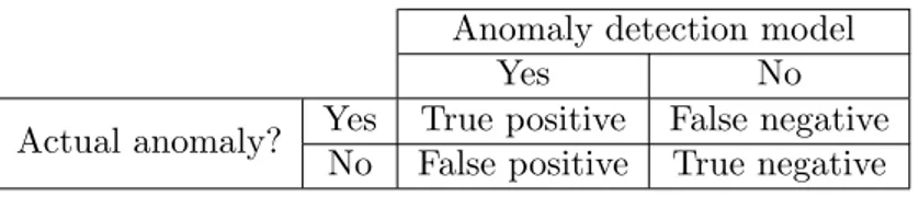
In order to determine whether a prediction or classification model is performing well, the following three metrics are commonly used; Precision, Recall and F-measure [9, 25]. To understand these it is necessary to keep count of how many times a prediction or classi-fication is right or wrong, in comparison to actual values [9]. Table 1 illustrates how to categorize right and wrong classifications in comparison to actual anomalies in a data set. This type of table is called a confusion matrix. If an actual anomaly has been classified as an anomaly, it equals a true positive, and if an actual data point is not an anomaly and is not classified as one, it equals a true negative. Inaccurate classifications of anomalies, for instance if a model classifies an anomaly where there actually is not one, equals a false positive. In the same way, a false negative occurs when the model classifies a data point as not an anomaly while it actually is an anomaly.
Table 1: Illustration of how to determine true or false positives, as well as true or false negatives, when analyzing the outcome of a classification model made for anomaly detection.
Anomaly detection model
Yes No
Actual anomaly? Yes True positive False negative No False positive True negative
Precision is defined as the number of true positives (TP) over the number of true positives plus the number of false positives (FP), as shown in the following formula [26]. It can be described as the veracity of detected anomalies actually being anomalies, and not false anomalies [27].
Precision = TP
TP + FP (13)
Recall is defined as the number of true positives (TP) over the number of true positives plus the number of false negatives (FN) [26] as shown in formula 14. Another word for describing recall can be completeness [27], which presents how many of the actual anomalies could be identified by a specific model.
Recall = TP
F-measure considers both precision and recall to calculate the score as a weighted average, defined by formula 15. This score varies between 0 and 1, where 1 is the best value [9].
F-measure = 2 × Precision × Recall
3
Related work
This chapter presents summarized versions of previous work related to this thesis. Each presentation concludes with how it is relevant to this thesis.
3.1 Data driven modeling for energy consumption prediction in smart buildings
In this paper, Gonz´alez-Vidal et al. [5] proposed a machine learning approach in which black-box models, i.e. data-driven models, were used in order to predict energy consump-tion. The aim was to evaluate whether a state-of-the-art black-box method could show better prediction accuracy than a grey-box method, i.e. a combination of physics based and data-driven models.
The development and training of the proposed model was based on data collected through-out one year, from February 2016 to February 2017. The building chosen for this study was the Chemistry Faculty of the University of Murcia. When developing the black-box model, several relevant algorithms were implemented for comparison; Support Vector Re-gression (SVR), ReRe-gression Forest (RF) and Extreme Gradient Boosting (XGB).
The results of this study showed that a black-box model using the Random Forest al-gorithm outperformed the rest. Both the mean absolute percentage of error (MAPE) and the coefficient of variation of the root mean squared error (CVRMSE) of the model were outstanding compared to the rest. The proposed model was able to capture the human behavior better than both the regression-based electricity load model and the Gaussian model.
This paper presents and compares different approaches for developing a model with the purpose of predicting energy consumption in smart buildings. Due to the paper presenting several possible algorithms it is a relevant source of information for this thesis.
3.2 Design and implementation of an open-source infrastructure and an intelligent thermostat
The work of Loumpas et al. is presented in this paper [6] where a hardware and software system for smart management of a building heating system is described. This work aimed to set a new protocol for interconnecting all the registered IoT devices of a building, by creating a central hub.
The bibliography research on the related subject for this paper revealed the lack of open source implementation. This resulted in the decision to make the details of the work, both regarding software and hardware, publicly available. For the proof of concept, a smart thermostat was developed and tested in a house located in Kastoria, Greece. The thermostat was managed through the application server which was set up on a raspberry Pi. This experiment was conducted from September to December of 2017.
The results presented a unified control system managing a smart thermostat that is said to train automatically during its usage, while improving its predictions. Through the support by the application server, the smart thermostat operated over two separate tasks. The first task conducted sampling of temperature in relatively small intervals. The second task was the core of the smart thermostat. Here an analysis was performed of the samples from the first task, and a data-set was produced. This data-set was what the smart thermostat op-eration was based on, when scheduling a desired temperature at a certain time for example. Although the objective of this paper was somewhat off topic when proposing a whole IoT control system, it has relevance to this thesis. Not only does the paper present a smart thermostat with the ability of making predictions but it also refers to the solution details which are available to the public though GitHub. The open source is rare for these types of solutions.
3.3 A low-complexity control mechanism targeting smart thermostats
The objective of this paper by Danassis et al. [4] was to introduce a low-cost but high-quality Decision Making Mechanism (DMM) for smart thermostats. By incorporating Artificial Neural Networks (ANN) and Fuzzy Logic, a person’s thermal comfort was im-proved while maintaining the total energy consumption. An ANN was proposed to make the computing of temperature set-points fast yet accurate. Then, Fuzzy Logic was im-plemented in order to take into account inherent constraints posted at real-time, such as trading price of energy. Due to having this combination of ANN and Fuzzy Logic, DMM supports the task of smart temperature regulation while actively participating in the en-ergy market. It does this by facilitating the usage of renewable resources, batteries and dynamic energy pricing policies. If a home would have numerous renewable power sources available, the DMM could determine whether to buy energy from the main grid or use the self-generated renewable energy. In case the availability of renewable sources exceeds the demand, the DMM decides whether it is optimal to store it in battery or sell it to the grid.
The experimental setup consisted of five neighborhood buildings equipped with a number of weather sensors collecting data throughout a five month period, from May to Septem-ber. In favor of minimizing energy costs, rechargeable batteries were employed, as well as photovoltaic panels. The framework was evaluated by a detailed simulation of a micro-grid environment of buildings located in Chania, Greece. Historic weather data and energy pricing was used for simulation. A hardware prototype was then developed for the DMM. The algorithm chosen for training the ANN during this development was the Levenberg-Marquardt back-propagation algorithm. It was chosen because of its increased perfor-mance, especially for non-linear regression problems.
The introduced DMM resulted in higher thermal comfort values but it also accomplished to redistribute energy in a way that considerably improved the total cost. The solution derives close to optimal results without the need of historical data or weather forecasts. In comparison to a couple of existing control techniques, this solution was placed at the
top, without being as complex or time demanding as the existing techniques.
When developing an algorithm as the one this thesis aims to propose, this paper presents an inspiring source of solutions. Although the scope of this paper is wider, taking different energy sources into consideration, it has presented a lot of theory relevant for this thesis.
3.4 Implementation of Machine Learning Algorithm for Predicting User Behavior and Smart Energy Management
In this paper, Rajasekaran et al. [28] implement a Machine Learning algorithm for pre-dicting the energy usage of a house hold. This was accomplished by feeding back the energy usage data of each appliance back to the controller. A GUI was also developed for empowering the user.
The Machine Learning algorithm presented in this paper was developed by combining the Nearest Neighbor Algorithm and the Markov Chain. As the proposed solution needed to find similarities between the state of each appliance (ON/OFF), the Nearest Neighbor algorithm was considered a good fit. Based on the transitions between states, points were distributed by implementing Markov Chain algorithm.
The results of the proposed solution showed that flattening of load curve was possible by never allowing controllable loads to switch ON during peak hours of energy consump-tion. Controllable loads refer to the devices whose time of use is not important to the user. The GUI for the solution made the user more informed and empowered by the wide range of functions it offered.
The information presented in this paper is relevant to this thesis because of its detailed description of how to develop the proposed machine learning algorithm. Although the focus extends to multiple devices and a GUI, parts of the report could inspire this thesis.
3.5 Analysis of energy and control efficiencies of fuzzy logic and artificial neural network technologies in the heating energy supply system responding to the changes of user demands
This paper by Ahn et al. [29] presents controllers implementing the Fuzzy Inference Sys-tem (FIS) and Artificial Neural Network (ANN) for simultaneously controlling air supply and its temperature in response to changes in demand.
The testing was conducted on one reference model and six control models, and a sim-ulation was generated in MATLAB. The simsim-ulation was performed under the conditions of temperature at Raleigh Durham Int’l Airport derived from EnergyPlus weather data. Each simulation was performed under two scenarios for set-point temperature; fixed and changed.
During simulation with fixed set-points, most controllers indicated high control efficiency. When the simulation tested the controllers in the scenario of changing set-points, most
controllers showed high control efficiency in comparison to the conventional thermostat. The results show an advantage in the ANN controller’s efficiency in preventing energy consumption for heating from rising more than 4%. In the scenario of changed set-point, the ANN controller was exceptionally efficient in suppressing heating energy consumption increasing by less than 1%. Both the FIS and the ANN models had advantages over the typical ON/OFF baseline controller when it comes to control efficiency directly related to human comfort.
The analysis of controllers for heating systems in this paper makes it a relevant infor-mation source for this thesis. Both the choice of algorithms as well as the choice of conditions and tools for simulation could be valuable for this thesis.
3.6 Probabilistic reasoning for streaming anomaly detection
In this paper, Carter and Streilein [21] present a Probabilistic Exponentially Weighted Moving Average (PEWMA) for anomaly detection in network security. By dynamical adjustment of parameters based on the probability of a given observation, the proposed method produced data-driven anomaly thresholds which were robust to data anomalies yet quick to adapt to distributional data shifts, unlike Exponentially Weighted Moving Average (EWMA).
As an extension of EWMA, having an exponentially decreasing weight factor (α), this paper introduced an additional probabilistic weight (β) to the moving average of the pre-vious samples. (1−βP ), where P is the probability, was chosen to be placed as a weight on α. That way, the samples that were less likely to have been observed offer little influence to the updated estimate. The development of this model was performed using a data set of reported global intrusions in network security, provided by the SANS Internet Storm Center. For the experiment, a training period of 14 days was set for both EWMA and PEWMA, and β, which was only used for PEWMA, was set to 1. The threshold θ was set to alert observations exceeding 3 standard deviations from the predicted value, thus detecting any anomalies.
The results of this work show that, when it comes to the prediction mean squared er-ror per day, PEWMA outperformed EWMA for all α values. PEWMA was also better at predicting the data with a lower standard deviation. Although EWMA was quicker to react to the first abrupt burst in the data set, it was not as sufficient as PEWMA when it came to adjusting the threshold. This resulted in EWMA missing several anomalies after the first, while PEWMA quickly recovered and detected these anomalies.
The method for anomaly detection presented in this paper could be suitable for this the-sis. As this paper presents an algorithm for implementing a Probabilistic Exponentially Weighted Moving Average, it could be adapted for this thesis’ temperature data set.
3.7 Automatic Anomaly Detection in the Cloud Via Statistical Learning
The work of Hochenbaum et al. [25] present two novel statistical techniques for automatic anomaly detection in cloud infrastructure data. The two proposed methods employ
sta-tistical learning and are referred to as Seasonal-ESD (S-ESD) and Seasonal-Hybrid-ESD (S-H-ESD).
The data used in this work was a wide collection of time series data obtained from pro-duction, using metrics such as heap usage, application metrics and tweets per minute, etc. The evaluation used over 20 data sets ranging from two-week long periods to four-week long periods. S-H-ESD with an α-value of 0.05 was used for anomaly detection, run over a time series containing the last 14 days worth of data. The efficiency of ESD and S-H-ESD, regarding capacity engineering, user behavior and supervised learning were each evaluated by reporting the precision, recall and F-measure of each method, combined with the size of the α-value used.
The results showed that the S-H-ESD method, with the highest F-measure of 17.5%, 29.5% and 0.62% for capacity engineering, user behavior and supervised learning respec-tively, outperformed the S-ESD method.
This paper is relevant for this thesis because of its experimentation with moving aver-ages while developing the methods presented in the paper. This is theoretically relevant for developing the solution that this thesis aims to present.
4
Method
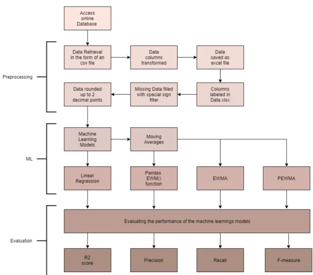
This chapter presents the research methodology used during this thesis. Since the thesis aims to develop four different algorithms the Nunamaker methodology [30] was chosen.
4.1 Method description
Nunamaker research methodology was chosen due to it describing development as an iterative form. As figure 3 portrays, the methodology consists of five different stages used to be repeated in order to achieve a fully functional system.
Figure 3: A research process of systems development research methodology.
4.1.1 Construct a conceptual framework
As the first stage of the iterative development process its purpose is to generate ques-tions that are to be solved. These quesques-tions are known as research quesques-tions and are formed by comprehending the research domain and understanding its research problems. As mentioned these questions are dependent on knowledge of the research domain and therefor change during the course of the thesis (see section 1.2.2, Research Questions). This knowledge is accessed by conducting a literature study in order to study the scope of which the problem is part of. Examining the initial thesis proposal in combination with group discussions, with the help of a supervisor these question first take form.
4.1.2 Develop a system architecture
Stage 2 of this iterative process is about defining functionality, not just for the entire system but also for its subsystems. By understanding the limitations of the system (see section 1.3, Limitations), functionality can be established. As a whole it is important to showcase the functionalities and how they relate to one another and for that reason, a system architecture was created, presented in figure 4.
Figure 4: A figure of the System architecture, displaying all subsections of the problems that this thesis consists of.
4.1.3 Analyze and design the system
During this stage it is important to evaluate the first 2 stages of the process. By analysing subsystems which are put forth, several different solutions to these are thought out. All being suited for implementation, the purpose of this stage is to analyze and single out the most optimal solution. This is done by examining the limitations of the system and the aim of this thesis. These factors are then evaluated to bring forth which solution that would be the better one out of the chosen ones.
4.1.4 Build the prototype
The fourth stage is about taking the optimal solution found in the previous stage and implementing it. For this thesis this will consist of implementing and further tweaking the chosen methods. The chosen methods, Linear Regression, pandas own EWM function, an original EWMA function and a PEWMA algorithm, are explained in section 2, Theory.
These different types of algorithms will be implemented for future use of temperature data from IoT sensors setup in Karlshamn, Sweden,
4.1.5 Observe and evaluate the system
Being the fifth and last stage of the process, this stage is used to verify the entire sys-tem. As mentioned previously in order to confirm and evaluate their ability to meet the requirements. This is done by ensuring that the fourth stage has completed and the dif-ferent algorithms are available for testing. By using temperature data the algorithms will try and detect anomalies in the temperature data set that differ from the rest according to theory presented in section 2.3, Outlier Detection. The evaluation is based upon the algorithms ability to detect anomalies and their accuracy, which is evaluated using the metrics described in sections 2.5, R2 statistic scoring model, and section 2.6, Precision, Recall and F-measure. The anomaly detection for Linear Regression is tested by identify-ing errors beyond the scopes of set thresholds. The anomalies and their accuracy are to be documented and presented in tables in the thesis. In the case of pandas EWM function, an original implementation of EWMA and the further modified EWMA, PEWMA, the anomalies are detected by the thresholds (the thresholds are presented in section 5.1.3, Anomalies). This detection is based on that EWMA or PEWMA values intersect with thresholds, giving off an alert that a value is far lower or higher than expected and therefor an anomaly.
5
Results
The following subsection, Result Introduction, will display all necessary information re-garding the results. This includes the choice of environment for development, the pre-processing of the data set and how anomalies are defined. This is followed by the chosen weight parameters for certain models that were tested and how their performance is eval-uated.
All graphs for Linear Regression, Pandas EWM function, EWMA and PEWMA are based off of the data set collected from apartment 2. This is done to showcase the difference in results between the different models and how well they perform on the same prerequisites. However, all tables display results from all 9 apartments for greater accuracy regarding the calculated scores for the different models tested.
5.1 Result Introduction
5.1.1 Environment for Development and Testing
Choice of environment for developing the machine learning algorithms is Python 3.6. During the first stage of the research methodology, construct a conceptual framework, the choice was made as it was deemed the most suitable for this thesis. The accessibility to open source repositories such as pandas and numpy is a convincing factor for it being the choice of environment. Scikit is another repository which allows for usage of their easy implementable tools regarding certain machine learning algorithms, such as Linear Regression.
5.1.2 Data set
This thesis was built on a data set of different weather variables that are being collected in a building in Karlshamn, Sweden. The building has an IoT system set up for gathering information such as humidity, indoor temperature, outdoor temperature and even received signal strength indicator (RSSI). However, this thesis was limited to data sets containing temperature variables, this limitation is brought up in the first chapter, 1.3 Limitations. The building has been monitored for over a year with sensors that update the value of the room temperature and store it in a database [31]. This database is accessed online and the data is retrieved in the form of a comma separated values file, also known as a csv file. On retrieval the file consists of three columns. Column 1 has the time and date for when the temperature value was collected. Column 2 is a label, a string that has both the apartment from which the temperature value was collected but also the specific room the sensor was placed in. The third column is the important one, it contains the temperature values that are considered the data. The first issue with the data upon access to it was that all temperature values were stacked within a single column. Meaning that if there are five temperature values retrieved, and the apartment has six sensors, then all five tem-perature values for all six sensors are placed in the same column, yielding 30 values in a single column. The first step of preparing the data, or preprocessing it, was to transform this single massive column into several columns where each column was representative of
the values from the room they were collected. An empty row of cells was inserted at the top of each file, allowing for labeling of the columns, such as labeling the column for the kitchen as ”TempK”. An example of this can be found Appendix A, a figure describing the column transformation.
The data was saved as excel files with temperature variables in five to seven columns in each file, depending on apartment, specifically within the range of the columns [2,6,10,14,18,22,26]. Appendix A includes a picture of the columns, as labels of the columns, that are available in each apartment for extraction. Last part of preprocessing the data was to ensure that there were no values missing. This was done by applying a special sign filter to the whole excel file stating that if any value was to be missing, it is to be automatically filled with the previous value above it. This measurement was taken to avoid conflict in code as missing values would be considered as NaN, Not a Number values, which would cause errors when using the value for calculations with other floats.
Each temperature column consists of a label with its name, followed by 672 measured and stored values. These represent temperature values collected every 15 minutes, indi-cating a data set with collected values over the period of one week. This is true for all data sets regarding all 9 apartments, that are used for testing in this thesis.
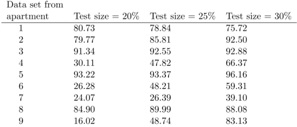
The results for table 4, in section 5.2, Linear Regression, are obtained by using a method called ”train test split” in order to divide the data set into four parts. The target depen-dent variables as its training data, and the independepen-dent targets’ variables as its training data. The two remaining parts are test data that consists of various amounts of data from the full data set. As seen in table 4 (section 5.2, Linear Regression), the test size varies and implies the size of the split test data. However, the approach was then improved by removing the ”train test split” functionality in order to use the whole data set. This due to the results from table 4 and the implication that more data leads to more reliable results with a higher R2 score.
5.1.3 Anomalies
According to theory, presented in section 2.3, Outlier Detection, an anomaly is a pattern in the data that does not conform to expected normal behavior. The normal behavior of the data set used during this thesis was defined as the region within the thresholds applied to the moving average (for pandas EWM, EWMA and PEWMA). An anomaly was detected whenever a data instance exceeded these thresholds.The thresholds were set to 0.5 as this resulted in the models detecting the highest number of predefined anomalies. The anomaly thresholds work similarly for Linear Regression, but they are not prede-fined. Linear Regression anomalies are calculated by applying Linear Regression on a data set. The difference between the calculated Linear Regression and the original data set value is then considered a error. Displaying this difference in a histogram, is a way of showing the distribution of errors. The histogram will then show how most Linear Regression values lie within the same range of errors. Leading to a visual representation of values that are out of the norm, furthest from the normalized distribution and therefor
considered as an anomaly in this thesis.
Table 2: The amount of predefined anomalies in each apartments own data set. These anomalies have been predefined through visual inspection by the authors of this thesis.
Apartment 1 2 3 4 5 6 7 8 9 Total
Number of predefined anomalies 1 3 0 8 4 11 1 8 8 44
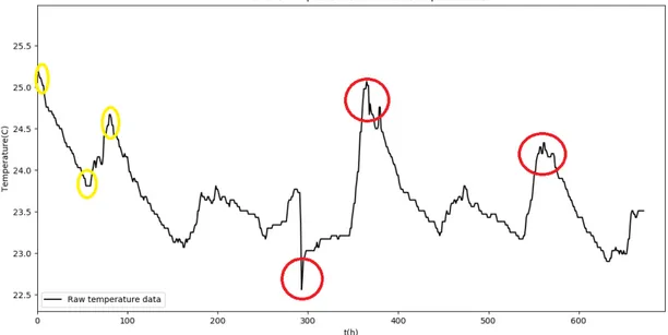
The predefined anomalies showcased in table 2 are determined graphically by displaying temperature values in each apartment. These predefined anomalies are defined due to the values of the temperature being either too high or too low compared to the average. In figure 5 the raw data set for apartment 2 is displayed due to it being the apartment all displayed tests are tested on. As seen in table 2, the number of predefined anomalies in apartment 2 is three. These three anomalies can be seen in the figure below, marked by red circles. The yellow circles could be anomalies but because of their position in the data set they are not considered as such. This is due to the ramp up time of the chosen methods, and that their ability to correctly calculate the newer values increase after a handful of iterations. This can be observed in the EWMA method, where the build up time for the method can be seen in figure 9 in section 5.4, EWMA.
Figure 5: Figure displaying the raw data from apartment 2. Red circles are predefined anomalies and yellow are excluded due to reasons presented in section 5.1.3, Anomalies.
This was done to all data sets, and anomalies were defined for the determination of the accuracy in regards to anomaly detection of all models after they have been tested. The total amount of predefined anomalies in the data sets is 44. However, the models can predict several anomaly points at each predefined anomaly. This is due to the fact that an anomaly can occur over a time period containing several data instances of the time-series data set. Both anomaly points and the number of found anomalies in the data set will be presented in the tables for all tested models. In the context of this thesis and the
predefined anomalies, the possibility of a true negative anomaly is non existent. This will be represented in the confusion matrices as a 0 for all results.
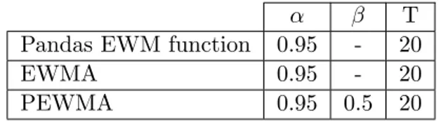
5.1.4 Weight parameters
The moving averages of Pandas EWM function, the EWMA model as well as the PEWMA model were weighted using alpha and the period T, but also an addition of beta to the PEWMA model. The values applied for these parameters during the work of this thesis were the ones presented in table 3.
Table 3: The weight parameters used for each model.
α β T
Pandas EWM function 0.95 - 20
EWMA 0.95 - 20
PEWMA 0.95 0.5 20
5.1.5 Accuracy
The accuracy of each anomaly detection model was evaluated using the metrics Precision, Recall and F-measure (described in section 2.6, Precision, Recall and F-measure). Addi-tionally, the R2 statistic score (described in section 2.5, R2 statistic scoring model) was used to evaluate the fit of the Linear Regression model.
The results present a confusion matrix for each model displaying the accuracy in terms of true or false positives and negatives, respectively. From these, the precision as well as the recall of each model was determined. In order to determine which model possessed the optimal balance between precision and recall, the F-measure of each model was calculated.
5.2 Linear Regression
Table 4 is a depiction of the accuracy for the Linear Regression. The table shows the accuracy for the different apartments with varying amounts of data from the data set, set aside for training. The data set for Linear Regression consists of data collected over a week from several apartments.
Table 4: The R2of the Linear Regression algorithm for all apartments and a varying portion of
the data set used for testing.
Portion of data set assigned for testing Data set from
apartment Test size = 20% Test size = 25% Test size = 30%
1 80.73 78.84 75.72 2 79.77 85.81 92.50 3 91.34 92.55 92.88 4 30.11 47.82 66.37 5 93.22 93.37 96.16 6 26.28 48.21 59.31 7 24.07 26.39 39.10 8 84.90 89.99 88.08 9 16.02 48.74 83.13
Observing the results from apartment 1 through 9 in table 4, over the course of 1 week, the overall performance in regards to the R2 improved. This is due to the fact that more data was available for testing. Once this had been achieved by the ability to calculate predicted values using the data set, an error calculation was the next step.
Et= Ppred− Dt (16)
By plotting the errors, the distribution of errors can be seen as a histogram in figure 6.
Figure 6: Histogram displaying the distribution of errors.
Plotting the errors enables for an analysis of the distribution in order for reasonable thresholds to be set. The thresholds can then be used to compare with errors that are beyond their scope. Specifically in accordance with figure 6, natural thresholds can be observed at Et = -0.75 and Et = 0.75. Errors beyond these thresholds are classified as
anomalies and stored as such. This will allow for them to be plotted as scatter points to make notice for anomalies along the raw data. This can be seen in figure 7 below, the red points are points that could potentially be anomalies detected by the linear regression method.
Figure 7: Anomalies plotted as scatter points in a continuous graph displaying temperature over a period of time.
This can be applied to all data across all apartments for a comparison of both the number of anomalies as well the R2 score. The score along with the number of anomalies detected by the Linear Regression model can be seen in table 5.
Table 5: The R2 of the Linear Regression algorithm for all apartments, the amount of points
that could be anomalies, and the amount of anomalies.
Apartment R2score Anomaly Points Number of Anomalies
1 78.5 14 1 2 91.86 28 2 3 94.9 25 3 4 75.7 14 5 5 98.8 11 2 6 89.5 17 5 7 47.4 13 1 8 89.7 17 2 9 98.35 9 1
Table 5 shows the number of anomalies and for showcase purposes, figure 7 can be exam-ined as at x values close to 100 and 300, two anomalies can be seen. However, at roughly x = 370, the biggest anomaly point in all of the plot is seen and has not been detected as an anomaly. This indicates that for this data set specifically, 2 out of 3 anomalies
were detected. Taking this further and including all data sets, further results could be determined as a confusion matrix based on anomalies was created.
Table 6: Confusion matrix of the anomaly detection model using linear regression. The total amount of actual anomalies is 44.
Once this confusion matrix was established, the known values of true positives and neg-atives, and their false counterparts could be established. These values were then used to calculate the precision of the Linear Regression model and the recall of the model. Having both precision and recall, the F-measure score for Linear Regression for the temperature time series data set could be calculated.
Table 7: The accuracy of the Linear Regression model in terms of precision, recall and f-measure.
Precision Recall F-measure
81,8% 45% 58,1%
5.3 Pandas EWM function
The implementation of Pandas EWM function for anomaly detection was tested on the same data set as for all the models and with the parameter settings described in section 5.1, Result Introduction. Figure 8 presents the results of this anomaly detection, graphically.
Figure 8: Illustration of Pandas EWM function detecting anomalies in the indoor temperature data set, that exceed the thresholds during a week in April.
By analyzing figure 8 the number of anomalies detected is obviously two, although the model discovered several anomaly points to each anomaly. As this specific data set contains three predefined anomalies, this model totally missed one of them. Table 8 presents the exact number of anomalies (and anomaly points) detected by this model, for each apartment’s data set during the same time period.
Table 8: The amount of points in the data registered as anomaly points and the total amount of anomalies detected in the plot using pandas own EWMA function.
Apartment Anomaly Points Number of Anomalies
1 8 1 2 14 2 3 0 0 4 29 8 5 10 3 6 52 7 7 11 1 8 5 2 9 54 4
From these results a confusion matrixs was created to display the number of true or false positives, as well as the true or false negatives. This is presented in table 9.
Table 9: Confusion matrix of the anomaly detection model using Pandas EWM function. The total amount of actual anomalies is 44.
To evaluate the performance of this model, the results from the confusion matrix were further used to calculate the metrics Precision, Recall and F-measure, presented in table 10.
Table 10: The accuracy of the Pandas EWM function in terms of precision, recall and f-measure.
Precision Recall F-measure
50% 46.7% 48.3%
5.4 EWMA
The EWMA model was implemented and then tested using the same conditions (see section 5.1, Result Introduction) as the rest of the models. Figure 9 illustrates the results of the anomaly detection using this model.
Figure 9: Illustration of the EWMA model detecting anomalies in the indoor temperature data set, that exceed the thresholds during a week in April.
As the illustration in figure 9 shows, two out of three predefined anomalies were detected. In the case of EWMA there is a build up time for the method as seen in the graph, leading to data values exceeding threshold values which according to the algorithm are considered as anomalies. This is expected and is only to be ignored as it has zero impact on anything later on and that the method quickly stabilizes. All detected anomalies discovered by this model are presented in table 11.
Table 11: The amount of points in the data registered as anomaly points and the total amount of anomalies detected in the plot using an implemented EWMA algorithm.
Apartment Anomaly Points Number of Anomalies
1 48 1 2 51 2 3 36 0 4 69 8 5 49 3 6 80 9 7 47 1 8 42 2 9 97 4
Based on table 11, a confusion matrix was created illustrating the true or false positives, as well as the true or false negatives the model produced. This confusion matrix is presented in table 12.
Table 12: Confusion matrix of the anomaly detection model using EWMA. The total amount of actual anomalies is 44.
The performance of the EWMA model was further evaluated in terms of Precision, Recall and F-measure, displayed in table 13.
Table 13: The accuracy of the EWMA model in terms of precision, recall and f-measure.
Precision Recall F-measure
66.6% 58.8% 62.5%
5.5 PEWMA
Using the same conditions as for all the previously presented models, PEWMA was tested and figure 10 illustrates the performance of this model. This final model was the only one to detect all three predefined anomalies of this specific data set.
Figure 10: Illustration of the PEWMA model detecting anomalies in the indoor temperature data set, that exceed the thresholds during a week in April.
All anomalies detected by the PEWMA model are presented for each apartment in table 14.
Table 14: The amount of points in the data registered as anomaly points and the total amount of anomalies detected in the plot using an implemented PEWMA algorithm.
Apartment Anomaly Points Number of Anomalies
1 24 1 2 32 3 3 2 0 4 53 9 5 29 4 6 94 11 7 36 1 8 28 5 9 82 6
From these results, a confusion matrix was created for the PEWMA model, displaying the amount of true or false positives, as well as the true or false negatives. This confusion matrix is presented in table 15.
Table 15: Confusion matrix of the anomaly detection model using EWMA. The total amount of actual anomalies is 44.
Finally, the evaluation metrics Precisoin, Recall and F-measure were calculated to deter-mine the accuracy of this PEWMA model. These are presented in table 16.
Table 16: The accuracy of the PEWMA model in terms of precision, recall and f-measure.
Precision Recall F-measure
6
Analysis and Discussion
6.1 Method Discussion
We chose to work according to the method of Nunamaker and Chen’ methodology [30], throughout this thesis. It allowed for a structured work flow that allows for flaws to be rep-rimanded when found. This iterative process was helpful when stumbling upon unknown errors or mistakes that forced us back a stage or two in the process. When implementing PEWMA and coming to the realization that certain calculations and formulas were prin-cipally wrong, we could take a step back to an earlier stage and re-evaluate them. The strength of the methodology is in its later stages when iteration becomes critical. Not being able to change and fix that which does not work, hurts a project and is one of the reasons why waterfall development was avoided. The Nunamaker and Chen methodology really helped break down this thesis for us and put it into different subsections for better clarity and overall understanding of the project. The different stages that build up the Nunamaker and how it structured this thesis is detailed in chapter 4, Method.
6.2 Data set Analysis
The data set consists of temperature values from a total of nine different apartments being observed for temperature data gathering. We made the choice to use all nine apartments for testing instead of focusing on a single apartment. We believed that being able to do the same tests, on different data sets collected during the same time period would produce better results.
Following this decision, the data sets were extracted from the online data base. The data sets retrieved were for temperature values for the period of April 2018 through April 2019. The more data available, would only lead to better results as the different methods would have more variables to be tested on. However, we chose to lessen the period of the data sets because of these several reasons.
• Algorithm run time • Moving averages • Seasons
When using a data set containing temperature values from a whole year, there were 17520 rows of values for each sensor. This puts each file at containing either 87600, 105120 or 122640 temperature variables. This inherently meant two things, first being that the initial run time of extracting the variables into python was far too long. The second part being the iterations of calculations that followed, being too long which would lead to un-necessary time consumption.
The second reason was straight forward due to that moving averages only consider sub-sections of data sets for calculations. For Pandas EWM, EWMA and PEWMA, whether it was a year of data or a week was arbitrary. But there was another disadvantage for using a data set of a full year. In the case of Linear Regression, using a data set filled
with temperature values from a whole year, the calculated line would have a big offset. This would be the output due to the temperature values being collected over different seasons. Temperatures during the winter season differ a lot from the temperatures during the summer. This would produce a Linear Regression model with higher values of error. These error values would be in violation of the threshold values and thus also the prede-fined anomalies in this thesis leading to faulty results. For these reasons, the temperature data sets were reduced to a period of 1 week and 672 temperature values per room with a sensor.
6.3 Result Discussion
After implementation and evaluation of four different models for anomaly detection during this thesis, we found that PEWMA was best suited for time-series temperature data sets. With a precision of 80% and a recall of 88.8% it scored the best F-measure of 84.3%, outperforming the other models. Table 17 shows the accuracy metrics for each model, previously presented in sections 5.2 through 5.5.
Table 17: The accuracy of each tested model in terms of precision, recall and f-measure.
Precision Recall F-measure
Linear Regression 81.8% 45% 58.1%
Pandas EWM 50% 46.7% 48.3%
EWMA 66.6% 58.8% 62.5%
PEWMA 80% 88.8% 84.3%
Although the Linear Regression model performed better than the other models in terms of precision, having the highest percentage of 81.8%, it also had the lowest recall percentage of 45%, out of the four models. This low recall could be caused by the poor fit of the Linear Regression model. The reason to why it is a poor fit, is because of its inconsistency of the R2 score which can be found in table 5, section 5.2. As a result, the F-measure for Linear Regression was 58.1%, thus better than Pandas EWM but not as accurate as EWMA or PEWMA.
Note that when analyzing the results of Pandas EWM function with our own implementa-tion of EWMA, our implementaimplementa-tion is clearly better. Our EWMA model scores a precision of 66.6% compared to Pandas EWM which got the poorest precision of 50%. With a recall of 58.8%, EWMA is still better compared to the recall of Pandas EWM model, being only 46.7%. As a consequence, our EWMA model scores a higher F-measure as well, having a score of 62.5% compared to the 48.3% of Pandas EWM. These results expose the Pandas EWM function as the least suitable model, out of the tested models, for anomaly detection on a time-series temperature data set.
Looking at the number of predefined anomalies of each apartment, presented in table 18 and in section 5.1.3, Anomalies, it is clear that PEWMA outperforms the other three models by detecting 32 out of the 44 predefined anomalies. The other models, EWMA, Linear Regression and Pandas EMW were able to detect only 20, 18 and 14 anomalies, respectively. The PEWMA model was the only one to detect all predefined anomalies of
apartment 2 and apartment 5.
Table 18: The results of how many of the actual, predefined anomalies each model could detect.
Number of predefined anomalies detected by model
Apt. Number of
predefined anomalies Linear Regression Pandas EWM EWMA PEWMA
1 1 1 1 1 1 2 3 2 2 2 3 3 0 0 0 0 0 4 8 5 5 6 5 5 4 2 1 2 4 6 11 4 2 5 9 7 1 1 1 1 1 8 8 2 0 0 4 9 8 1 2 3 5 SUM 44 18 14 20 32
The results were produced by applying specific parameters to the models, as described in section 5.1.4, Weight parameters. The weighted multiplier alpha, also referred to as the smoothing parameter, was experimented with before deciding that a value of 0.95 was the best fit. After several experiments with different alpha-values, varying between 0 and 1, the value of 0.95 was the one resulting in a smooth graphical representation of the model. The beta parameter, which is a weighted multiplier, was set to 0.5 when testing our PEWMA model. A value of 0 would change the PEWMA model to a EWMA model, and a value of 1 would result in more drastic reactions to abnormal data. Therefor we chose a stable value of 0.5 to our beta parameter.
The period, T, used for each model during this thesis was set as 20, representing a time frame of 5 hours. After several experiments using different time periods this was the best fit. A smaller value to this parameter would not achieve a moving average as good as the one generated by the T being 20, because the average would only represent a really small period of time with minimal changes in the temperature. If the T parameter was set too high it would on the other hand result in taking the average of a too long time frame, loosing the ability to detect possible anomalies within the time frame.
In the result sections for all models, the tables presented anomaly points as well as the number of anomalies. As discussed and seen in figures and tables, the number of anoma-lies can be directly tied to the way we measured performance for all models in this thesis. However, as described in section 5.1.3, Anomalies, there are also anomaly points that have a correlation with the number of actual anomalies. Meaning these could also be an indication of how well or how bad a model is performing. As we have not come across a metric for anomaly points, we can still see that there is a clear correlation between anomaly points that are related to predefined anomalies. This is visually easy to see as

![Figure 2: An illustration of a contextual anomaly in a temperature time-series. The temperature at time t 1 is the same as the temperature at time t 2 , but it is only considered an outlier in the later context [18].](https://thumb-eu.123doks.com/thumbv2/5dokorg/4045560.83230/13.892.189.717.367.627/figure-illustration-contextual-anomaly-temperature-temperature-temperature-considered.webp)