Are commuter train timetables consistent with passengers’ valuations of waiting times and in-vehicle crowding?

Are commuter train timetables consistent with passengers’

valuations of waiting times and in-vehicle crowding?

VTI Working Paper 2020:1

Abderrahman Ait-Ali

_{, Jonas Eliasson}

_{and Jennifer Warg}

1

_{Transport Economics, VTI, Swedish National Road and Transport Research Institute}

_{Communications and Transport Systems, Linköping University}

3

_{Transport Planning, KTH Royal Institute of Technology}

Abstract

Many models have been developed and used to analyse the costs and benefits of transport

investments. Similar tools can also be used for transport operation planning and capacity allocation.

An example of such use is the assessment of commuter train operations and service frequency. In this

study, we analyse the societally optimal frequency for commuter train services. The aim is to reveal

the implicit valuation (by the public transport agency) of the waiting time and the in-vehicle crowding

in the commuting system. We use an analytic CBA model to formulate the societal costs of a certain

service frequency and analyse the societally optimal frequencies during peak and off-peak hours.

Comparing the optimal and the actual frequencies allows to reveal the implicit valuations of waiting

time and crowding. Using relevant data from the commuter train services in Stockholm on a typical

working day in September 2015 (e.g., OD matrix, cost parameters), we perform a numerical analysis

on certain lines and directions. We find the societally optimal frequency and the implicit valuation of

waiting time and crowding. The results suggest that the public transport agency in Stockholm (i.e.,

SL) adopted service frequencies that are generally slightly higher than societally optimum which can

be explained by a higher implicit valuation of waiting time and crowding. We also find that the

optimal frequencies are more sensitive to the waiting time valuation rather than that of crowding.

Keywords

Waiting time; Crowding; Cost benefit analysis; Implicit preference; Commuter train

JEL Codes

1. Introduction

Public transport is a central part of most urban transport systems, and the decisions of public transport agencies about which services to run are hence very important. In this paper, we explore to what extent timetables determined by a local public transport agency (PTA) are consistent with passengers’ valuations of waiting times and in-vehicle crowding, by analysing the timetables’ trade-offs between these variables and the operations costs of train services. Just as passengers’ valuations can be inferred by observing their choices between travel options, analogous implicit valuations can be derived from the choices which the agency makes when determining timetables. These implied valuations can then be interpreted as the agency’s revealed preferences regarding e.g., waiting times and crowding. The question is then whether these coincide with passengers’ valuations. Similar studies of the implicit preferences of public agencies have been conducted by e.g., McFadden (1975), McFadden (1976), Nellthorp and Mackie (2000) and Eliasson and Lundberg (2012), studying PTAs’ choices of infrastructure investments and revealing implicit valuations of different kinds of benefits and costs. To our knowledge, this is the first similar study of an agency’s timetable decisions.

There are several reasons why this question is important. First and most obvious, possible differences between agencies’ and passengers’ implicit valuations raise several interesting questions. Is the agency simply failing to construct cost-efficient timetables? In that case, the methods developed in this paper can indicate how such timetables can be improved. Or is there something missing from the conventional benefit-cost framework, that the agency (correctly) considers? Or are the agency’s decisions perhaps affected by other considerations – perhaps (hidden) political pressure? Or are there some constraints on the agency’s decisions which prevent it from making optimal decisions from the passengers’ point of view? Exploring whether an agency’s decisions are consistent with passenger valuations forms a starting point for interesting and deep discussions about an agency’s objectives and efficiency, as well as the ability of cost-benefit analysis (CBA) to capture the relevant aspects of public transport service provision.

A second motivation for our interest in this issue is that it has been suggested by Johnson and Nash (2008) and Ait Ali et al. (2020) that CBA of timetable adjustments can be used to resolve capacity conflicts between commercial and local (publicly controlled) commuter trains. The idea is to calculate the net loss of social benefits of adjusting a commuter train timetable to make room for a commercial train service, and use this loss as a reservation price for the commercial train slot: capacity is allocated to the commercial train if a commercial operator is willing to pay an access charge equal to this reservation price. However, this idea rests on the assumption that the CBA framework used to calculate the social loss from the timetable adjustment is consistent with the PTA’s timetable preferences. If not, the idea might be difficult to accept for the PTA– for example, if the results of the cost-benefit analysis would indicate that it would yield a positive net social benefit to reduce the number of commuter train services compared to what the agency wants. At least, one would need to investigate the reasons for possible differences between the valuations in the CBA framework (based on passengers’ valuations) and the preferences of the PTA, and determine whether or how they can be reconciled.

A third reason for investigating the principles underlying agencies’ timetable choices is that knowledge of these principles is necessary for evaluating infrastructure investments. As discussed in Eliasson and Börjesson (2014), the benefits of a railway capacity improvement are determined by the difference in timetables with and without the investment. To conduct a CBA of a railway investment, these timetables must hence be constructed, and the analyst needs a guiding principle to determine them. Eliasson and Börjesson (2014) suggest that, in the lack of better evidence, an analyst could assume that the PTA strives to maximize net social benefits – but empirical evidence of the principles implicit from agencies’ actual timetable choices is obviously better.

The current paper demonstrates the use of cost benefit analysis to optimise the frequency of a commuter train service. It also contributes with an alternative valuation perspective of waiting time and (in-vehicle) crowding different than the passenger perspective. The paper has the following structures: section 2 provides an overview of the relevant research literature. Section 3 describes the analytic model. Data for the numerical analysis is presented in section 4 and the corresponding results in section 5. We conclude the paper with section 6.

2. Literature Review

There is a vast literature on passengers’ valuations of trip dimensions, such as in-vehicle travel time, crowding, waiting time, walking time and delays. Abrantes and Wardman (2011) provide an overview and meta-analysis based on British evidence. Wardman and Whelan (2011) also performed a meta-analysis study to evaluate the

British value of crowding in rail trips. The two authors collected data on crowding valuations from the last 20 years from 15 different studies. The meta-analysis quantified the variations in the large set of time multipliers. The study aggregated these values into implied multipliers for seated and standing travellers for commuter and leisure trips. Most such valuation studies are based on stated choice experiments, but there are also studies based on observed behaviour, for example Tirachini et al. (2016) who estimate crowding valuations (standing and sitting multipliers) based on smart card data from the metro system in Singapore.

For the purpose of this study, Swedish valuation studies are of course most relevant. The valuation of waiting time is based on the Swedish value of time study, reported in Algers et al. (2010) and Börjesson and Eliasson (2012), and subsequently included and updated in the Swedish CBA guidelines (ASEK, 2018). We use a valuation of crowding obtained in Björklund and Swärdh (2017), who estimated crowding multipliers for different modes and areas based on Swedish data, reaching similar results as the Wardman and Whelan (2011) meta-study.

Just as passengers’ implicit valuations can be inferred by analysing their choices between options with different benefits and costs, agencies’ implicit preferences can be inferred by analysing their decisions. One of the earliest such studies is McFadden (1975) who looked at the implicit valuations of benefits and costs of road infrastructure investments implied by a transport agency. The author developed a theoretical framework based on discrete choice modelling to infer the implicit choice criteria (i.e., parameter valuation) that was adopted by the government bureaucracy for the investment selection. The inference relies on actual ex-post evaluation of the consequences and outcomes of the selection decisions. The quantitative model allows to estimate the government’s revealed implicit valuation on selection criteria.

Basu (1980), in a book about the revealed preference of governments, attempts to set an early formalisation of the model by Weisbrod and Chase (1968) that studied the income redistribution weights in CBA studies. This formalisation is based on a standard model for social welfare function and the distinction between local and global welfare. Such a model allows to estimate the weights in the welfare function based on information about the projects that were chosen by the government. Another formalisation by the same author was the use of fuzzification for analysis of revealed binary preferences (Basu, 1984). Brent (1991) discussed the previous techniques for revealing the government distributional weights. The author contrasted the stochastic methods, e.g., McFadden (1975) with the deterministic ones, e.g., Basu (1980) indicating a preference for stochastic methods, namely Probit technique. The latter is applied and discussed in the case of the UK railway closure at that time. This same preferred stochastic approach is also used in the more recent work by Scarborough and Bennett (2012). They applied choice modelling techniques to estimate distributional weights in CBA models for environmental policy analysis. Compared to the many studies of travellers’ valuations, there are only a few studies of the implicit preferences of bureaucracies, such as PTAs. Even fewer have compared the two sets of valuations, and as far as we know none in the context of public transport planning (e.g., commuter train systems). A number of studies look at the optimal supply of public transport such as the study by Qin and Jia (2013) on a crowded rail transit line in China and a more recent study by Asplund and Pyddoke (2019) on bus services in a small Swedish city. Such works do not further study the implicit valuation of any of the trip parameters. However, there are some studies (outside of public transport supply) that compare consumer (i.e., personal and self-interested) and citizen (i.e., social and moral) preferences. Im et al. (2014) looked at the extent to which citizen preferences are reflected in the resource allocations from the budget of the city of Seoul both at city and district level. The authors find that there is no perfect reflection of such preferences, meaning that resource or budget allocation in the city seem to be non-participatory. The authors highlight and discuss the potential of a participatory budgeting which reflects the citizen preferences. Similar studies were also conducted in the US (Franklin and Carberry-George, 1999), the Netherlands (Michels and De Graaf, 2010) and Malaysia (Manaf et al., 2016). Most of these studies claim the positive impact of citizen involvement in decision making, and that participatory decision making is highly desirable in representative democracies. However, Bossert and Weymark (2004) find it difficult to include all the citizen groups and show that the social welfare maximising function can be dictatorial. Therefore and according to Arrovian social choice theory, certain individual preferences must be considered over the others, see Arrow's impossibility theorem or paradox (Arrow, 1963).

Lewinsohn-Zamir (1998) criticises the distinction between consumer and citizen preferences in the context of the provision of public goods, e.g., public transport services. The author claims that such a distinction is unrealistic, and no quantitative difference can be made, arguing that both preferences are driven by other trade-offs that are less manifested in daily life. Moreover, since such preferences are successfully considered, in many cases, in the political arena, citizen preferences should be given more weight and be carefully used in tools such cost-benefit analysis.

3. Analytic model

Our evaluation framework includes passenger benefits and train operations costs. Passenger benefits include travel times, in-vehicle crowding and waiting times, while operations costs include fixed costs, time- and distance-dependent costs and overhead costs. Since we are studying relatively minor changes in the timetables, we use a fixed origin-destination matrix, which means that there are no changes in external effects, such as noise and emissions, due to modal shift from road transport, and no changes in fare revenues or tax revenues (e.g., from fuel taxes). These effects can hence be omitted from the analysis.

In the present study, we also ignore unexpected delays. This is an important issue for future research, since delay robustness (minimizing knock-on delay effects from incidents) may be an important consideration when constructing timetables. As we shall see, however, this omission does not seem to affect our main conclusions in the present paper.

Consider a commuter train line and direction with a fixed passenger origin-destination matrix, and let the service frequency be 𝑁 trains per hour. Given an origin-destination matrix and a service frequency 𝑁 trains per hours, the number of boarding and alighting passenger on each station can be calculated. Let 𝐵𝑖𝑘 and 𝐴𝑖𝑘 be boarding/alighting

passengers at station 𝑖 and service 𝑘 (we distinguish directions by letting stations have different indices depending on which direction passengers are travelling in, so each physical station will have two indices, one for each direction of the line). Let 𝐹𝑖𝑘= ∑ (𝐵𝑙≤𝑖 𝑙𝑘− 𝐴𝑙𝑘) be the number of passengers onboard train service 𝑘 at the link

following station 𝑖.

The total societal cost 𝑇𝐶(𝑁) for the services is the sum of passengers’ generalized travel costs and operating costs for the train services. Generalized travel costs consist of two parts: waiting times and in-vehicle travel times. The valuation 𝛽 of waiting time (i.e., headway between services) is assumed to be constant, since we study high-frequency services; for low-high-frequency services, the marginal valuation of headway decreases, since travellers can often adjust their schedule to avoid waiting at the platform. The valuation of in-vehicle travel time increases with the crowding in the vehicle, since traveling in crowded conditions incurs a higher disutility per minute on travellers. Let the valuation of in-vehicle time be 𝛼 (1 + 𝛾 (𝐹𝑖𝑘

𝑆) 𝜃

), where 𝛼, 𝛾 and 𝜃 are parameters, 𝑆 is the number of seats

in the train and 𝐹𝑖𝑘 the number of passengers onboard train service 𝑘 on link 𝑖. Operating costs include personnel,

maintenance and other operation costs. We ignore fixed costs since they do not vary with the service frequency. Total societal costs of the train services, formulated in equation (1), are obtained by summing operation costs 𝐾𝑁, waiting time costs Σ𝑖𝑘𝛽

𝐵_𝑖𝑘

2𝑁 and in-vehicle time costs (weighted by crowding) Σ𝑖𝑘𝛼 (1 + 𝛾 ( 𝐹_𝑖𝑘 𝑆) 𝜃 ) 𝑡𝑖 𝐹𝑖𝑘:

TC(𝑁) = 𝐾𝑁 + ∑ 𝛽

1

2𝑁

𝐵

+ ∑ 𝛼 (1 + 𝛾 (

𝐹

𝑆

)

) 𝑡

𝐹

(1

)

It is possible to rewrite equation (1) by rearranging the terms that include the frequency. The reformulation of the societal costs 𝑇𝐶 is given in equation (2).

TC(𝑁) = 𝐾𝑁 + 𝛼 ∑ 𝑡

𝐹

+

𝛼𝛾

𝑆

∑ 𝑡

(𝐹

₎

+

𝛽

2𝑁

∑ 𝐵

(2

)

Note that the term ∑𝑖,𝑘𝑡𝑖𝐹𝑖𝑘 is the total passenger-travel time which is constant and does not depend on the level

of supply (i.e., frequency). Another constant term is ℬ: = ∑𝑖,𝑘𝐵𝑖,𝑘 which is the total number of passengers boarding

the system. The optimal service frequency 𝑁∗ _{is the one that minimises total societal cost:}

𝑁

= 𝑁

(𝛾, 𝛽, 𝜃) = argmin

𝑁∈ℕ∗

TC(𝑁)

(3

)

If crowding is ignored (𝜃 = 0), we obtain the formula for the optimal frequency in equation (4) or the well-known square root principle stated by Mohring (1972). If the crowding penalty is linear in seating occupancy (𝜃 = 1), the optimal frequency becomes (denoting the in-vehicle crowding term by ℱ𝜃=1):

𝑑TC

𝑑 𝑁

(𝑁

_{) = 𝐾 −}

𝛽ℬ

(𝑁

₎

= 0 ⇒ 𝑁

= √

𝛽ℬ

𝐾

(4

)

𝑑 TC

𝑑 𝑁

= 0 ⇒ 𝑁

_{= √}

𝛽ℬ + 𝛾ℱ

𝐾

(5

)

The study of the analytic expression of the optimal frequency for general values of 𝜃 can yield very complex analytic formulations. In some cases (e.g., integer values 𝜃 ≥ 4), there is no possible closed form (Abel, 1824). Therefore, we explore the optimal frequency using a numerical approach, and also use it to study the effects of the valuation parameters on the optimal train frequency.

Table 1

Values that are used for the parameter valuation in producer and consumer costs (10 SEK ≈ 1 EUR).

Parameter Value Reference

Travel time 𝛼0= 65.5 SEK per hour

Average travel time valuation (57 SEK/h) for leisure and (74 SEK/h) for commutes (Eliasson and Börjesson, 2014). Waiting time 𝛽₀= 80 SEK per hour

We assume that the average waiting time is less than 10 min and consider the average valuation by Algers et al. (2010) between leisure (86 SEK/h) and commuting (74 SEK/h).

Crowding 𝛾0= 0.085

𝜃0 = 3

Using results by Björklund and Swärdh (2017) from stated preference crowding valuation study in Stockholm (and two other large cities in Sweden), a curve fitting of the crowding function 1 + 𝛾 (𝐹𝑖𝑘

𝑆) 𝜃

was performed to find 𝛾 and 𝜃. Operation

𝐾𝑑𝑖𝑠𝑡𝑎𝑛𝑐𝑒= 30 SEK/wagon-km

𝐾𝑡𝑖𝑚𝑒= 5 205 SEK/wagon-h

𝐾𝑜𝑣𝑒𝑟ℎ𝑒𝑎𝑑= 9 %

All parameter values for the producer costs are from (SLL, 2017). The fixed costs are 5.000.000 SEK per year-wagon, we therefore consider the fixed costs per hour assuming each wagon is operated 6 hours per day and 260 days per year.

Table 1 presents the adopted values (column 2) for the different cost parameters (column 1) as well as the references to the original studies (column 3). The travel parameters (𝛼, 𝛽, 𝛾, 𝜃) are all indexed with 0 to reflect that the adopted values are from specific studies of the Swedish travel parameters. The seating capacity of a commuter train (with two coupled trainsets) is 𝑆 = 748 seats in total (ALSTOM, 2004). Most of the trains during the studied time intervals are operated with two wagons even during mid-day (off-peak) due to other considerations such as infrastructure restrictions and punctuality, even though passenger loads are much lower. For comparison, we also analyse optimal off-peak frequency assuming operations with short trains (single trainset, 𝑆 = 374). Moreover, note that the valuations are from different years and may need harmonisation to a common year.

4. Data

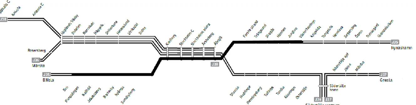
In this section, we present the input data for the numerical analysis performed on a commuter train line from Stockholm. Fig. 1 presents the commuter network (as of 2015) and the studied line (filled in black). We first study the part of the J35 line between Kungsängen (Kän) and Västerhaninge (Vhe). The line includes 17 stations (from a network total of around 50) with Stockholm central station as the largest passenger station. Part of the studied line (i.e., between Karlberg and Älvsjö) are shared with other lines (e.g., J38 and J36) that will later be studied and compared with the main studied line.

For each pair of stations, we know the number of trips in every 15 minutes over a normal day in September 2015, i.e., the time-dependent OD matrix, from smart card data. Fig. 2 illustrates the number of passengers entering each station per 15 minutes interval over the day.

A similar distribution is also available for the number of passengers alighting in each station per time interval. Given a certain train timetable (i.e., frequency), both distributions are used to calculate the number of passengers

boarding

𝐵

𝐴

𝑘

𝑖

𝐹

𝑘

𝑖,

The trip distribution that is used in this study is from a normal working day. The distribution can substantially vary from one working day to the other and find a normal (or typical) day can be challenging. Therefore, given the availability of the trip distribution data over several days, it is recommended to consider an average distribution. This is not the case in this study as we do not have such data.

Travel times between stations 𝑡𝑖 are known and constant. We study three main time intervals: morning peak

(6:00 – 9:00), afternoon peak (15:00 – 18:00) and mid-day off-peak (10:00 – 13:00).

The local public transport agency in Stockholm (SL) adopted in 2015 the commuter train timetable (i.e., frequency) presented in Table 2. It shows the actual service frequency from Kungsängen to Västerhaninge, including extra departures on parts of the line during peak hours.

Fig. 1. Studied (filled in black) line of the commuter train network in Stockholm, adapted from (SLL, 2015).

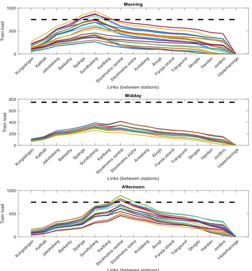
Fig. 3. Estimated number of passengers onboard trains from Kän to Vhe during different time intervals. Each line shows

passenger loads for one service from first to last station.

Table 2

SL's service frequency from Kän to Vhe for different time intervals during a working day.

Time interval Nb. regular departures

(per hour) Nb. extra departures (per hour) Total departures (per hour) Morning peak (6:00 - 9:00) 41 ₃2 _7.0 Mid-day off-peak (10:00 - 13:00) 4 - 4.0 Afternoon peak (15:00 - 18:00) 4 2 6.0

Using the total frequency and trip distribution, it is possible to estimate the total number of passengers onboard each train from Kungsängen to Västerhaninge for the different studied time intervals as illustrated in Fig. 3. Note that the horizontal dashed line refers to the total number of seats in a two-wagon train, i.e., 𝐾𝑐𝑎𝑝= 748 seats

(ALSTOM, 2004). Note that we also consider the passengers boarding (and alighting) from (and to) transfer trips from the OD-matrix. It is also important to note that since we study part of the whole line from Kungsängen to Västerhaninge, we assume that all trips, before Kungsängen, board from that first station. The same assumption applies for passengers alighting after last station Västerhaninge.

There is a regular service frequency during all the studied time intervals, see column 2 in Table 2. Trains serve parts or run beyond the studied line. However, peak hours include additional or extra train departures which are 1 _{Certain trains are running parts or beyond the studied line, e.g., to Älvsjö or Nynäshamn, from Jakobsberg.} 2 _{The provided frequency for extra departures is an average since not all are regularly running every X minute.}

not all regular. There are 9 departures in total during morning peak (i.e., every 20 minutes in average) and 6 departures in the afternoon (i.e., every 30 minutes), see column 3 in Table 2. Those extra departures, as the regular ones, do not operate the whole line but for the sake of simplicity, we assume they do which leads to the total frequency presented in column 4 of Table 2.

5. Results

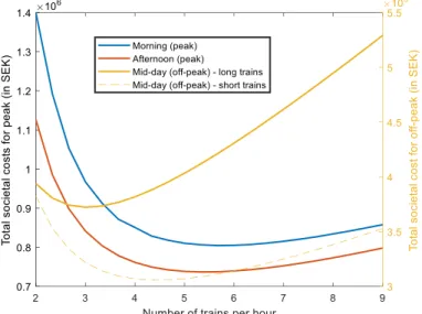
Given the input data and the method for calculating total societal costs presented above, we can calculate the total societal cost as a function of service frequency (trains per hour) for different time intervals: morning, mid-day and afternoon. For the mid-mid-day time interval, both long and short trains are presented with the corresponding total costs with a scale on the right y-axis.

Fig. 4. Total societal costs as a function of the frequency for different time intervals.

The total societal cost has a minimum which corresponds to the socially optimal frequency, given the parameters assumed above. A higher frequency than the optimal leads to operating costs larger than passenger benefits, whereas a lower frequency than the optimal leads to passenger costs increasing faster than savings in operating costs. The numerical values for the optimal frequencies in the different time intervals are reported in the second column in Table 3, and compared to the public transport agency’s actual frequencies.

Table 3

Comparison between the actual and the socially optimal train service frequency (trains per hour), given valuation parameters assumed in Table 1.

Time interval Optimal frequency (in trains/h) SL’s frequency (in trains/h)

Morning 5.7 7.0

Mid-day – long trains 3 4.0

Mid-day – short trains 4.3 -

Afternoon 5.3 6.0

The actual frequencies by the transport agency in Stockholm (i.e., SL) are slightly higher than the optimal ones, given the valuation parameters assumed in Table 1. Based on these parameters, the public transport agency should reduce the service frequency on this line and direction. But this result can also be interpreted as the agency putting a higher implicit valuation on either waiting time, crowding or both than the valuations assumed in Table 1. We thus turn to the question of identifying the agency’s implicit valuations, as implied by the choice of timetable.

For the sake of comparison, we study the societally optimal frequency on other lines and directions. In addition to the opposite direction of the studied line (i.e., from Vhe to Kän), we also look at the line between Upplands

Väsby (Upv) and Tumba (Tu) in both directions (i.e., southwards and northwards), see Fig. 1. The results are

Table 4

Comparison of the optimal frequency on other lines and directions.

Time interval

SL

Kän → Vhe

(Southwards)

Vhe → Kän

(Northwards)

Upv → Tu

(Southwards)

Tu → Upv

(Northwards)

Morning

7.0

5.7

5.7

6.7

7.3

Mid-day (long trains)

4.0

3.0

3.3

3.3

3.3

Mid-day (short trains)

-

4.3

5.0

5.3

5.3

Afternoon

6.0

5.3

5.7

6.7

6.3

As for the main studied line and direction (i.e., Kän to Vhe), the societally optimal frequency on the other lines and directions is generally slightly lower than the actual frequency by SL. The exceptions are in the afternoon peak hour on the line between Upv and Tu in both directions as well as in the morning peak hour from Tu on the same line. These are the only cases where SL is running fewer trains than optimum. Such higher optimal frequencies on these lines and directions is mainly due to the higher ridership which requires running more trains to reduce waiting time and crowding costs.

Note that using shorter trains during off peak hours always leads to a higher optimal frequency than SL’s, especially on the line Upv and Tu. The latter has a generally higher optimal frequency which is mostly due to the cheaper production costs (for shorter trains) justifying higher frequencies with higher ridership.

From an operational point of view, the frequency for the two directions on the same line should be similar. This constraint can be satisfied in different possible ways. For instance, the line frequency could be set as the average or maximum of the two optima. Another alternative is to modify the model in order to include all the line (i.e., both directions) with a single variable for line frequency. Further modifications to the latter to include the other line(s) allow to find the optimal service frequency in the network (if set to be the same for all the lines). However, such modifications require accounting for the transfer costs.

In what follows, we focus on the main studied line and direction (i.e., Kän to Vhe) to illustrate the implicit valuation of waiting time and crowding. Similar method can be used to study the other directions and lines.

5.1. Valuation of waiting time

The waiting time valuation 𝛽 affects the optimal service frequency. The fact that the actual frequency is higher than the optimal one calculated based on the parameters from Table 1 (𝛽0= 80 SEK/hour) implies that the

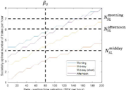
agency’s implicit valuation is higher than 𝛽0. Fig. 5 shows the variation of the optimal frequency when varying the

waiting time valuation 𝛽. The horizontal lines show the frequencies for morning, midday and afternoon whereas the vertical line relates to the stated preference value of 𝛽0.

As expected, we find in Fig. 5 that a higher waiting time valuation leads to a higher optimal frequency. If the actual frequencies for the different time intervals are projected on the axis for each curve, the corresponding x-axis projection values can be used to reveal the implicit valuation of waiting time. Table 5 presents the numerical values for the agency’s implicit valuations of waiting time for different time periods.

Table 5

The implicit waiting time valuation (𝛽0= 80 SEK/h).

Time interval Implicit waiting time valuation (SEK/h)

Morning 144

Mid-day (long trains) 144 Mid-day (short trains) 60

Afternoon 156

The agency’s implicit valuations in Table 5 are generally higher than passengers’ valuations (according to the studies CBA guidelines are based on), except for mid-day off peak hours if only short trains had been used. The valuations of waiting times implied by the agency’s choice of timetable is almost twice as high passengers’ own valuations, based on the studies and guidelines cited in Table 1. Note, though, that these are the implicit valuations obtained if only the waiting time valuation is changed, while the crowding valuation is kept constant. Next, we study the crowding valuation parameters.

5.2. Valuation of in-vehicle crowding

The crowding valuation depends on two variables, the factor 𝛾 and the exponent 𝜃. Fig. 6 presents optimal frequencies as functions of 𝛾 (left) and 𝜃 (right), ceteris paribus.

As expected, higher crowding valuations generally yield higher optimal frequencies. For mid-day (with long trains), there is no effect which is due to virtually negligible crowding levels. The numerical results revealing the implicit valuation of crowding are given Table 6 for peak hours. Off peak hours are not shown due to the negligible crowding levels during this time interval.

The implicit in-vehicle crowding valuation is more than twice as high as the one based on passenger valuations in Table 1. This is mainly due to the low crowding level in the commuter system.

Note, though, that our calculation is based on average seating occupancy, i.e., that passengers are spread evenly across the train. In reality, there are more passengers towards the ends of the trains. Since the crowding valuation is a nonlinear function of the seating occupancy, heterogenous occupancy along the train will increase the total crowding penalty, even more so if one also considers that more passengers will by definition experience high crowding than will experience low crowding (since there are by definition more passengers where there is higher crowding). The losses for high-crowding parts of the train will hence outweigh the benefits of the low-crowding parts. Later in this paper, we perform a sensitivity analysis to study the effect of varying seat capacity on the optimal frequency.

Table 6

Revealed implicit valuation of in-vehicle crowding during peak hours (𝜃0 = 3, 𝛾0= 0.085).

Time interval Implicit crowding factor Implicit crowding exponent

Morning 0.281 9

Fig. 6. Socially optimal train frequency as a function of the crowding parameter (left – factor, right - exponent)

Fig. 7. Joint analysis of crowding factor and waiting time valuation during morning and afternoon time intervals

Moreover, demand varies across days, and since the crowding valuation is nonlinear, the higher crowding penalties during high-demand days will outweigh the corresponding lower crowding penalties during low-demand days. Another sensitivity analysis is performed later in this study to look at the effect of varying the demand (i.e., OD matrix) on the optimal frequency.

5.3. Joint valuation of waiting time and crowding

In order to see the joint effect of crowding factor and waiting valuation, we study the variation of the optimal frequency when varying jointly these two parameters. Fig. 7 plots the results for (from left to right) morning and afternoon peak hours. The x-axis and y-axis show the value of the crowding factor 𝛾 and waiting time 𝛽, respectively. The contours show the level curves for the societally optimal frequencies (i.e., number of trains/h).

Fig. 7 shows that the sensitivity of the optimal frequency to the waiting time is much higher than to the crowding factor, i.e., level curves are almost vertical. This is explained once again by the low crowding in the train vehicles.

5.4. Sensitivity analysis

The results that were previously presented are based on the assumptions that the OD matrix is from a typical working day in winter season. However, day-to-day variations can happen and may lead to an increased (or decreased) number of passengers using the commuter system. To study these variations, we perform a sensitivity analysis on the OD-matrix.

Based on the already used OD matrix, we analyse the optimal service frequencies using OD matrix variants with +/- 10, 20 and 30 % of passengers boarding and alighting. The results are presented in Fig. 8 for the different lines and directions during afternoon time interval.

Fig. 8. Optimal frequency when changing the OD-matrix for different lines and directions during afternoon.

Fig. 9. Optimal frequency when changing the seating capacity for different lines and directions during afternoon.

The optimal frequency increases linearly when increasing the passenger demand. The variation is almost similar for the different lines and directions. The magnitude of the variation in optimal frequency is small compared to that of the passenger demand. For instance, a 30% increase in demand (OD matrix) would require only 17% increase in supply (frequency) from Vhe to Kän.

Previously, we also assumed that passengers are assumed to enter train wagons in a uniform way. However, passengers tend to choose wagons that are near the entrance (or exit) of the train station which leads to increased (or decreased) crowding in certain wagons (Fang et al., 2019).

One way to study this difference in crowding levels between wagons is to vary the available seating capacity compared to the total number of seats in the trains. We perform a sensitivity analysis on the available seating capacity by considering that it is +/- 10, 20 and 30 % of the total number of seats. Fig. 9 shows the results.

When decreasing seating capacity (e.g., shorter trains or unbalanced loads between train wagons), optimal service frequency increases almost linearly. The magnitude of such increase is small compared to the variation in seating capacity. A decrease of 30% in the number of seats would require an increase in frequency of 11% (from

Vhe to Kän).

The optimal frequency is less sensitive to the changes in available seating capacity compared to changes in OD-matrix. Fig. 9 indicates that the reduction in optimal frequency decreases for higher available seats whereas Fig. 8 shows that the increase in optimal frequency becomes substantial for larger positive change in OD-matrix, especially for already crowded lines and directions.

Both Fig. 8 and Fig. 9 are during afternoon time interval. Similar results can be found during morning peak hours. However, no significant impact is found when doing the analysis during off-peak hours.

5.5. Summary and discussions

Given the assumption that the public transport agency strives to provide train commuter services that minimise the societal costs, we have studied if this is the case. If not, we attempted to explain the differences by revealing the implicit valuation of waiting time and crowding.

Several assumptions were made before formulating an analytic model for the total societal costs of commuter train services. For instance, trains are assumed to be running according to the fixed schedule, i.e., no delays. Sensitivity analysis allowed to study two other assumptions, i.e., varying OD-matrix between days and crowding between wagons.

Moreover, given the mathematical complexity of such a model, we use a numerical approach to compute the optimal service frequencies for different time intervals, number of wagons, lines and directions.

The results reveal that the transport agency generally chooses a close to societally efficient service frequency. However, in some cases, significant anomalies or differences exist between the optimal and actual frequency which allowed to reveal an implicit valuation of waiting time and sometimes (on crowded trains) of in-vehicle crowding. The joint study of the two parameters shows that waiting time value has larger influence on the optimal frequency. PTA (or SL) should therefore be more careful when studying the waiting time valuation compared to the crowding value. In particular, they should use a more accurate and reliable value of waiting time valuation.

That these anomalies are explained by an implicit valuation of waiting time and/or crowding means that the PTAs seem to use these implicit valuations instead of the passenger (state or revealed) ones. However, the anomalies can also be explained by other (external) factors which drive the choice of the actual service frequencies. For instance, some railway infrastructure restrictions can hinder the transport agency from running more or shorter trains which leads to the adoption of inefficient service frequencies. Another example is the political influence on the decisions of the public transport agency which is not based on any cost benefit model. Most of these (external) factors can be seen as “incorporated” in the implicit valuations that the PTA seems to adopt in their choice of service frequencies.

6. Conclusions and Future Works

This study attempted to analyse the costs and benefits of the choice of commuter service frequencies using the parameters values based on passengers’ state preferences. The focus was on waiting time and crowding valuations as they are among the decisive factors for choosing the frequencies in large commuting systems.

From an analytic model of the total societal costs, we studied numerically the societally optimal frequency on one of the highly frequented lines in Stockholm commuter train system 2015. The results show that the local transport agency SL generally adopts a slightly higher frequency than the societally optimum (suggested by the cost-benefit model). This, in its turn, entails that the transport agency has a higher implicit valuation of waiting time and crowding than the one state by the passengers. Moreover, we reveal these implicit valuations and compare them to the adopted stated preference valuations. Finally, we also find that the choice of the optimal frequency should be driven by improvements to the waiting time rather than the crowding. Apart from the studied valuations of waiting time and crowding, there might be some other more subtle factors (e.g., political lobbying, labour laws, etc.) which can also lead to a different choice of frequency than optimum.

Such results have several policy implications on the different stakeholders, e.g., the transport agency and the passengers. On the one hand, the agency is required to justify the actual choice of service frequency and to explain any difference to the optimum that is suggest by cost-benefit analysis models. Moreover, such suggested non-optimality questions the effectiveness of the actual operational decisions (i.e., frequency). On the other hand, if the passengers’ preference is one of the main driving powers in the decision process, their broad participation in stated or revealed preference studies is required for broader representativity and more democratic choice by the transport agency.

As mentioned in the introduction, CBA can be used to solve conflicts between train path applications (Ait Ali et al., 2020). It is often assumed that the actual timetable for commuter trains is societally efficient. The results of this study show that such assumption may not hold, e.g., removing a certain commuter train path may lead to positive societal benefits. This assumption is also important when considering new infrastructure investments in which actual existing capacity is not efficiently used, e.g., railway infrastructure capacity.

The model in this study is not only applicable to public transport cases. It can also be used to study other transport systems (e.g., bus and metro) or public utilities and services. Another possible use of the analytic model in this study is in train timetabling for local commuter services. It allows to study different timetabling strategies

such as periodic or cyclic. Line planning may also be studied where central parts of the network have more frequent trains as opposed to outer parts, and passengers have to makes transfers to travel between the two parts.

There are several possible extensions to the study. One is to consider all the commuter train network instead of analysing one line and direction. A second possible improvement is to consider additional performance measures, such as punctuality and interchanges. A third one can improve the model for the distribution of passengers in the trains which is considered here as uniform. Finally, provided data availability, the same analysis can be done using trip distributions from multiple days instead of a single typical working day.

Acknowledgment

This research is part of the SamEff project about socio-economically efficient allocation of railway capacity (samhällsekonomiskt effektiv tilldelning av kapacitet på järnvägar). The project is funded by a grant from the Swedish Transport Administration (Trafikverket). The authors are grateful to Roger Pyddoke and John Nellthorp for the valuable discussions and comments.

References

ABEL, N. H. 1824. Mémoire sur les équations algébrique: où on démontre l'impossiblité de la résolution de

l'equation générale du cinquième dégré, Librarian, Faculty of Science, University of Oslo.

ABRANTES, P. A. L. & WARDMAN, M. R. 2011. Meta-analysis of UK values of travel time: An update.

Transportation Research Part A: Policy and Practice, 45, 1-17.

AIT ALI, A., WARG, J. & ELIASSON, J. 2020. Pricing commercial train path requests based on societal costs.

Transportation Research Part A: Policy and Practice, 132, 452-464.

ALGERS, S., BÖRJESSON, M., SUNDBERGH, P., BYSTRÖM, C. & ALMSTRÖM, P. 2010. Valuation of Time in Transport – The National Studies 2007/08 in Sweden. WSP report.

ALSTOM 2004. CORDIA 60X Stockholm Transport Renews its Commuter Fleet. ARROW, K. J. 1963. Social choice and individual values.

ASPLUND, D. & PYDDOKE, R. 2019. Optimal fares and frequencies for bus services in a small city. Research in

Transportation Economics, 100796.

BASU, K. 1980. Revealed Preference of Government, Cambridge University Press.

BASU, K. 1984. Fuzzy revealed preference theory. Journal of Economic Theory, 32, 212-227.

BJÖRKLUND, G. & SWÄRDH, J.-E. 2017. Estimating policy values for in-vehicle comfort and crowding reduction in local public transport☆. Transportation Research Part A: Policy and Practice, 106, 453-472. BOSSERT, W. & WEYMARK, J. A. 2004. Utility in Social Choice. In: BARBERÀ, S., HAMMOND, P. J. & SEIDL, C.

(eds.) Handbook of Utility Theory: Volume 2 Extensions. Boston, MA: Springer US.

BRENT, R. J. 1991. On the estimation technique to reveal government distributional weights. Applied

Economics, 23, 985-992.

BÖRJESSON, M. & ELIASSON, J. 2012. The value of time and external benefits in bicycle appraisal.

Transportation Research Part A: Policy and Practice, 46, 673-683.

ELIASSON, J. & BÖRJESSON, M. 2014. On timetable assumptions in railway investment appraisal. Transport

Policy, 36, 118-126.

ELIASSON, J. & LUNDBERG, M. 2012. Do Cost–Benefit Analyses Influence Transport Investment Decisions? Experiences from the Swedish Transport Investment Plan 2010–21. Transport Reviews, 32, 29-48. FANG, J., FUJIYAMA, T. & WONG, H. 2019. Modelling passenger distribution on metro platforms based on

passengers’ choices for boarding cars. Transportation Planning and Technology, 42, 442-458. FRANKLIN, A. L. & CARBERRY-GEORGE, B. 1999. Analyzing How Local Governments Establish Service Priorities.

Public Budgeting & Finance, 19, 31-46.

IM, T., LEE, H., CHO, W. & CAMPBELL, J. W. 2014. Citizen Preference and Resource Allocation: The Case for Participatory Budgeting in Seoul. Local Government Studies, 40, 102-120.

JOHNSON, D. & NASH, C. 2008. Charging for scarce rail capacity in Britain: a case study. Review of Network

Economics, 7.

LEWINSOHN-ZAMIR, D. 1998. Consumer Preferences, Citizen Preferences, and the Provision of Public Goods.

The Yale Law Journal, 108, 377-406.

MANAF, H. A., MOHAMED, A. M. & LAWTON, A. 2016. Assessing Public Participation Initiatives in Local

MCFADDEN, D. 1975. The Revealed Preferences of a Government Bureaucracy: Theory. The Bell Journal of

Economics, 6, 401-416.

MCFADDEN, D. 1976. The Revealed Preferences of a Government Bureaucracy: Empirical Evidence. The Bell

Journal of Economics, 7, 55-72.

MICHELS, A. & DE GRAAF, L. 2010. Examining Citizen Participation: Local Participatory Policy Making and Democracy. Local Government Studies, 36, 477-491.

MOHRING, H. 1972. Optimization and Scale Economies in Urban Bus Transportation. The American Economic

Review, 62, 591-604.

NELLTHORP, J. & MACKIE, P. J. 2000. The UK Roads Review—a hedonic model of decision making. Transport

Policy, 7, 127-138.

QIN, F. & JIA, H. 2013. Modeling Optimal Fare and Service Provisions for a Crowded Rail Transit Line. Journal of

Transportation Systems Engineering and Information Technology, 13, 69-80.

SCARBOROUGH, H. & BENNETT, J. 2012. Cost Benefit Analysis and Distributional Preferences, Edward Elgar Publishing, Incorporated.

SLL 2015. Fakta om SL och länet 2015.

SLL 2017. SAMS 3.0 Documentation In: ADMINISTRATION, T. (ed.) Strategic Development of Socio-economic

Analysis. 2017-03-03 ed. Stockholm: Transport Administration.

TIRACHINI, A., SUN, L., ERATH, A. & CHAKIROV, A. 2016. Valuation of sitting and standing in metro trains using revealed preferences. Transport Policy, 47, 94-104.

WARDMAN, M. & WHELAN, G. 2011. Twenty Years of Rail Crowding Valuation Studies: Evidence and Lessons from British Experience. Transport Reviews, 31, 379-398.

WEISBROD, B. A. & CHASE, S. B. 1968. Problems in Public Expenditure Analysis. Washington, DC: The Brookings