V¨
aster˚
as, Sweden
Bachelor Thesis in Computer Science (15 Credits)
MACHINE LEARNING BASED
PEDESTRIAN EVENT MONITORING
USING IMU AND GPS
Davi Ajmaya
daa15001@student.mdh.se
Dennis Eklund
eds04001@student.mdh.se
Examiner:
Shahina Begum
M¨
alardalen University, V¨
aster˚
as, Sweden
Supervisor: Mobyen Uddin Ahmed
M¨
alardalen University, V¨
aster˚
as, Sweden
Abstract
Understanding the behavior of pedestrians in road transportation is critical to maintain a safe en-vironment. Accidents on road transportation are one of the most common causes of death today. As autonomous vehicles start to become a standard in our society, safety on road transportation becomes increasingly important. Road transportation is a complex system with a lot of different factors. Identifying risky behaviors and preventing accidents from occurring requires better under-standing of the behaviors of the different persons involved. In this thesis the activities and behavior of a pedestrian is analyzed. Using sensor data from phones, eight different events of a pedestrian are classified using machine learning algorithms. Features extracted from phone sensors that can be used to model different pedestrian activities are identified. Current state of the art literature is researched to find relevant machine learning algorithms for a classification model. Two models are implemented using two different machine learning algorithms: Artificial Neural Network and Hid-den Markov Model. Two different experiments are conducted where phone sensor data is collected and classified using the models, achieving a classification accuracy of up to 93%.
Contents
1 Introduction 5
1.1 Problem Formulation . . . 5
2 Background 7 2.1 Road transportation . . . 7
2.2 Sensors and Features . . . 7
2.3 Machine Learning . . . 8
2.3.1 Artificial Neural Network . . . 8
2.3.2 Hidden Markov Model . . . 9
3 Related Work 11 3.1 Feature Extraction, Selection and Classification . . . 11
4 Method 13 4.1 Data collection . . . 14
4.2 Feature extraction . . . 14
4.3 Ethical and Societal Considerations . . . 15
5 Implementation 16 5.1 Data collection and feature extraction . . . 16
5.2 Artificial neural network . . . 17
5.3 Hidden Markov model . . . 18
6 Results 20 6.1 Overview . . . 20
6.2 Experiment 1: Fixed window . . . 21
6.2.1 Artificial Neural Network . . . 21
6.2.2 Hidden Markov Model . . . 22
6.3 Experiment 2: Overlapping window . . . 24
6.3.1 Artificial Neural Network . . . 24
6.3.2 Hidden Markov Model . . . 25
7 Discussion 27 7.1 Limitations . . . 28
8 Conclusions 30 9 Future Work 31 References 33 Appendix A ANN Validation Confusion Matrices 34 A.1 Experiment 1: Fixed window . . . 34
A.2 Experiment 2: Overlapping window . . . 37
Appendix B HMM Validation Confusion Matrices 40 B.1 Experiment 1: Fixed window . . . 40
List of Figures
1 A representation of a fully connected ANN . . . 9
2 A representation of how a 1 layered CFNN is constructed taken from Mathworks . 9 3 A Markov Chain with two states . . . 10
4 Hidden Markov Model with hidden states and observable symbols . . . 10
5 Bin collection . . . 17
6 Representation of the architecture of Neural Network used to classify the different events . . . 17
7 A Hidden Markov Model implementation in MATLAB . . . 19
8 Multiclass confusion matrix example . . . 20
9 ANN confusion matrix on test set with 0% crossover . . . 22
10 HMM confusion matrix on test set with 0% crossover . . . 23
11 ANN confusion matrix on test set with 25% crossover . . . 24
12 HMM confusion matrix on test set with 25% crossover . . . 26
List of Tables
1 ANN sensitivity and specificity table with 0% crossover . . . 222 HMM sensitivity and specificity table with 0% crossover . . . 23
3 ANN sensitivity and specificity table with 25% crossover . . . 25
4 HMM sensitivity and specificity table with 25% crossover . . . 26
Acronyms
IMU Inertial Measurement Unit GPS Global Positioning System AI Artificial Intelligence
ML Machine Learning
ANN Artificial Neural Network
CFNN Cascade Forward Neural Network
HMM Hidden Markov Model
GMM Gaussian Mixture Model EM Expectation-Maximization
VA Viterbi Algorithm
CNN Convolutional Neural Network
MSE Mean Square Error
P Positive N Negative TP True Positive FP False Positive TN True Negative FN False Negative
TPR True Positive Rate
TNR True Negative Rate
PPV Positive Predictive Value NPV Negative Predictive Value
1
Introduction
Road transportation is a complex system that poses great challenges for todays society. In a report published by the European Commission1 in 2015, 90% of all crashes are caused due to the risky behaviors of different actors (e.g. vehicle drivers, motorcyclists, bicyclists and pedestrians). In 2015, the report states that 26 300 fatalities were reported in the EU, of which 22% were pedestrians, 15% were motorcyclists, 8% were cyclists and 3% were mopeds. Road accidents also cause serious injuries. In 2014, it was reported that 135 000 injuries occurred. For every reported death there are roughly four crippling injuries, eight severe injuries and 50 minor injuries. The social cost of the road fatalities and injuries is estimated to be of at least 100 billion in EU2.
To improve the road transportation safety, it is not sufficient to only analyze the risky behavior of the drivers, but also to do a collective behavior analysis of the other actors involved, such as pedestrians.
The possibility of being able to identify the different activities that a pedestrian is performing is valuable. To minimize the risk of accidents occurring it is critical to understand and identify the risky behaviors of pedestrians. Recent research has been done where classification models have been implemented using machine learning algorithms to identify different pedestrian activities. A survey done in 2017 compares different studies that have been done where models have been implemented, using different algorithms with different types of sensor data, that identifies different activity types for a person [1].
The aim of this thesis is to investigate and implement a Pedestrian model for different events using machine learning algorithms on data extracted from Inertial measurement unit (IMU) sensors and Global Positioning System (GPS) signals. Such model would be beneficial to identify the behaviors of pedestrian where risky behaviors would be observable. In order to achieve the desired goal, relevant data parameters will be researched that are needed in order to model the behaviors of a pedestrian. Current literature studies will be overviewed to identify relevant machine learning algorithms that can be used in the model. Two machine learning algorithms will be chosen and used in the implementation. A comparison of the two methods will be done and presented in the report.
This report is intended for anyone interested in the field. The following section will explain the problem formulation in more detail. Section 2 and section 3 will provide the reader with the necessary background information and state-of-the-art in order to understand the rest of the report. The following section will explain how the problem has been tackled. The implementation of the model will be described and the results will be presented. Furthermore, a discussion and a final conclusion of the study will be present at the end of the report.
1.1
Problem Formulation
Foreseeing and preventing accidents in road transportation is no easy task. Accidents happen because of many different variables, one being because of the risky behaviors of pedestrians. A safe environment in road transportation becomes even more important as the popularity of autonomous vehicles rises. To prevent an accident, we have to identify any potential risks in order to stop them before an accident occurs. To identify risks in a road transportation system, we have to first understand and identify the different types of events for the different actors involved. This thesis will focus on the different behaviors of a pedestrian in road transportation. The objective of this thesis is to model different events for a pedestrian with machine learning algorithms using IMU sensors and GPS signals. In order to achieve the desired objective, the following questions will be investigated:
• What features could be extracted from IMU sensors and GPS signals to model different events of a pedestrian?
1http://ec.europa.eu/transport/road_safety/pdf/vademecum_2015.pdf 2http://europa.eu/rapid/press-release_IP-16-863_en.htm
• Define different events of a pedestrian that can be identified using IMU sensors and GPS signals.
• How can a model be implemented using machine learning algorithms to identify the different types of events?
2
Background
Today, nearly everyone carries a smartphone with them everywhere they go. The average smart-phone today has IMU, GPS and magnetometers built in. This means that valuable data can easily be extracted and used as a tool to model the different behaviors of pedestrians. It also eases the process of integrating such a system into society since the information is widely available. A current subject where a lot of research and progress is being made are autonomous vehicles. Self-driving cars are rising in popularity and will no doubt be a part of the future. Having data and information of surrounding pedestrians accessible to the self-driving vehicles, to identify potential risky behaviors of the pedestrians, could significantly reduce the chances of accidents occurring. Many studies have been done researching the behavior of drivers in road transportation, but as Rangesh et al. [2] mentions, accidents do not solely occur due to the behavior of the drivers. Mod-elling pedestrians to better understand their behavior would enable us to identify risky behavior resulting in less accidents occurring.
2.1
Road transportation
An actor within road transportation is a person who is in some way apart of transportation on road. The combined activities of all actors define the road transportation and the action of every single individual actor affects the road transportation in some way. An actor may for example be a vehicle driver, bicyclist or a pedestrian.
An event is an activity that is performed by an actor. An event describes the behaviors of the different actors involved in a road transportation system. For a pedestrian, an event is an activity that a person can do while they are out on the street, such as walking, running, standing or stopping. In previous studies, the most common type of pedestrian events that have been studied are walking, running, standing and stopping [3,4,5,6,7,8].
2.2
Sensors and Features
The collected data is the information that can be extracted using built-in sensors, e.g. Inertial Measurement Unit (IMU) and GPS in a smartphone running an Android based operating system. To collect the data from the sensors on the phone, a third party application will be utilized to measure and store the sensor values. The third party application is called OARS - IMU & GPS Data Logger3which is made by KidTurbo and is available on Google Play. Some of the sensor values
that the application measures are the accelerometer, gyroscope, magnetometer, GPS location and gravity. The sensor data are then stored in a SQLite database file that can be transferred to a computer for further processing. The values stored in the SQLite file can then be transformed into features used to classify different pedestrian activities. The smartphone during the data collection will either be attached on the center of a subjects chest, in the front pocket of the pants or on a phone holder on the arm.
Inertial Measurement Unit (IMU) is a collection of accelerometer, gyroscope and magnetometer which typically is used to measure and track the kinematic of an object [9]. The accelerometer provides the acceleration in gravity of the X, Y and Z axis. This sensor data is the amount of gravity that is inflicted on the accelerometer tri-axes. The gyroscope provides the measurement of the angle for every axis. Angle information can be used to correct the data given from the IMU as the locations of the IMU axes change during movement. Global Positioning System (GPS) use satellites to capture the latitude and altitude of the devices position. This coordination can be used to find the position of the device and roughly calculate the speed of the pedestrian. GPS signals can be used as a complement to the IMU sensor data to correct variations and errors when calculating the speed [3].
Features are different types of behavior that can be observed using the collected data from the IMU and GPS. The features can be the raw data acceleration on each of the axes, peak-to-peak time, average acceleration, standard deviation, average resultant acceleration [10], step distance ∆Latitude and ∆Altitude [3].
2.3
Machine Learning
Artificial Intelligence (AI) is a field within Computer Science that studies the theory and devel-opment of computer systems to automate processes and activities that typically require human intelligence to perform. The field of AI studies the possibility of simulating the human intelligence on machines. Within the broad field of AI there are five major areas that are studied: perception, manipulation, communication, reasoning and learning [11].
Machine Learning (ML) is a subfield of AI. Machine learning focuses on the learning aspect of computer machines. The main objective of machine learning is to make machines to inherit the ability to learn [12]. This is typically done using statistical techniques. There exist a lot of different algorithms that work differently well depending on the problem. A group of machine learning algorithms are what is called classification algorithms. These algorithms utilize supervised learning [13]. Supervised learning based algorithms map an input to an output based on previous observations. Typically, these algorithms require training datasets that are used for the learning process of the algorithm. New data is then processed based on the prior gathered knowledge of the training dataset. A classification algorithm tries to identify what category a newly given input belongs to.
2.3.1 Artificial Neural Network
Artificial Neural Network (ANN) is a machine learning algorithm, which as described by Wang [14] is:
”Inspired by the sophisticated functionality of human brains where hundreds of billions of interconnected neurons process information in parallel, researchers have successfully tried demonstrating certain levels of intelligence on silicon. Examples include language translation and pattern recognition software.”
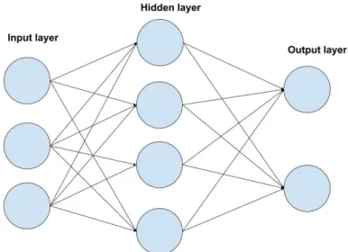
The neuron in the ANN consist of input signals, synaptic weights, linear aggregation, activation threshold or bias, activation potential, activation function and output signal [15]. Architecture of an ANN consists of layers of neurons, where each layer have one or more neurons. The basic structure is one input layer, any number of hidden layers and one output layer, this structure is shown in Figure 1. The output signal of each neuron is the summation of all the neurons Input signals x Synaptic weights and the total value of the summation inserted into the activation function. A common way to train an ANN is back-propagation which was used by Rangesh et al. to train the ANN [7]. By using the backpropagation algorithm the network is trained by hanging the weights on the connections using the error in the output layer. The Cascade Forward Neural network (CFNN) is made the same way as a feed forward network with fully connected layers, the difference is that in CFNN each layers output is connected to all the other layers as input. Figure 2 is a representation of a one layered CFNN taken from Mathworks documentation page on Cascadeforwardnet4. The
Cascadeforwardnet in MATLAB is trained using the Levenberg-Marquardt Algorithm.
Figure 1: A representation of a fully connected ANN
Figure 2: A representation of how a 1 layered CFNN is constructed taken from Mathworks
2.3.2 Hidden Markov Model
Hidden Markov Model (HMM) [16] is a machine learning algorithm that has its origin from the statistical Markov Model. Regular Markov Models utilizes Markov chains, which is a sophistic model with multiple states. The model describes the probability of events happening based on the previous state, where each state contains the probability of the model transitioning to another state. Figure 3 illustrates a Markov chain containing two states, and their respective probabilities of transitioning to the next state.
HMM uses the same principles, except for the fact that the states are hidden (i.e. unobserved). The model emits symbols (tokens) that represent observable data, which then can be analyzed. For every state in the model, there is an emission probability for every sequence of tokens. This means that the emitted tokens contain information that can be correlated with the states, even though they are hidden. HMM is most commonly used for recognizing speech patterns [17,18].
Figure 4 roughly displays the mechanism of a Hidden Markov Model where A represents the hidden states, B the emitted symbols and the arrows indicate the probability of transitioning from one state to another and the probability of emitting a symbol. Generally, when using a HMM, a system is described as having a finite amount of underlying states where transitions between these states occur according to a Markov chain. For every state, a symbol is emitted that represent observable
data. It is not possible to directly identify which state a model is, instead the identification is done based on the emitted (observable) symbols.
Figure 3: A Markov Chain with two states
Figure 4: Hidden Markov Model with hidden states and observable symbols
The observable input sequences can either be discrete (countable, quantized and finite) such as the results of rolling a dice or characters in an alphabet, or continuous (any value within a range) such as speech data, linear predictions or data collected from an IMU. To handle continuous data, it has to first be converted into quantized discrete symbols. However, a more common way is to use probabilistic models such as Gaussian Mixture Model (GMM) to represent the data [19].
When utilizing HMMs in different areas, three main problems may arise [16]. These three problems conclude:
1. Given a model and a sequence of observables (measurements), how can we calculate the probability of the sequence belonging to the model?
2. Given a model and a sequence of observables (measurements), how can we determine the sequence of states that best describe the sequence of observables?
3. Given a model, how can we optimize it to increase the precision of the probability for a sequence of observables (measurements)?
The most important points to consider when classifying a sequence of observables as a class k are problem 1 and 3. Essentially, to create a classifier using HMM a model has to be created for every class k that we want to classify. Each model should then be separately trained with data corresponding to the particular class. To test and classify a new sequence of data, the log-likelihood of the sequence belonging to each model is calculated. The sequence is then classified as the class for the model that produces the maximum likehood. This approach utilizes the Expectation-Maximization (EM) algorithm [19,20]. For problem 2, the Viterbi algorithm (VA) [21] is utilized. VA is an algorithm that estimates the most probable sequence of states that the model went through to produce a given sequence of observables.
3
Related Work
Previous research that studies the behavior of a person typically only studies a limited amount of events. These events are chosen and predefined before the experiments. For a pedestrian, the most common events have been monitored and studied in other research are walking, running/jogging and standing [2,3,4,5,6,7,8,10,22,23]. In some papers that have been published, other events such as sitting down, going up or down the stairs have also been studied [6,22]. These additional events however, are outside of our scope in this thesis. In a research done in 2012, the directions forward, backward, left and right are also taken into consideration when analyzing the walking behavior of a pedestrian. In the same paper, the event of turning around is classified as standing. However, in one of the studies, turning around is defined as a separate activity [4].
When data for the different events is collected, certain things such as locations and obstacles has to be taken into account. In a paper where the researchers study the behavior of pedestrians on sidewalk, they categorize the locations based on the width of the sidewalk, the amount of obstacles per 50 meters and how many pedestrians are walking on the sidewalk per minute [24]. Another method, used by Wells et al. [25] is to use a virtual environment where all the events are predefined. By using a combination of both of the previous data collection methods the events will have predefined conditions on the locations such as weather and traffic. The location on what body part the sensors are attached to will make a difference in how the values are changing during events. In an article published in 2011 by Arakawa et al. [26] the IMU system is attached to a helmet on the head, while researchers in another study [6,10] the sensors are located in the front leg pocket. Another method is to have the sensors attached on the chest which was used by two other studies [3, 22]. In some cases when data is being collected a camera is used to label time with the event [3, 7].
The IMU used in smartphones can give the accelerations of the X-axis, Y-axis and the Z-axis. The acceleration on the tri-axes of the IMU have been used in previous studies to detect the different activities that the subjects are performing [3, 6]. The most common way is to use only one IMU unit, but in some studies they are using multiple IMU units to be able to detect more complex activities such as reaching for objects or walking with a cane. In the study done by Nguyen et al. [4] 17 IMUs are utilized. With this many sensors a 17 point skeleton is created, this is similar to how it is done in other studies [2, 5] where a cameras are used to detect walking behaviors. In another study, GPS is used to calculate the velocity of the pedestrian, this velocity can be complimented with the dead reckoning method using the sensor values from the accelerometer [3]. The angles given from the gyroscope can be used correct the acceleration values to fit the rotation of the IMU [3], it can however also be used as a separate sensor value. The magnetometer is used to detect the orientation of the observed subjects.
3.1
Feature Extraction, Selection and Classification
By using a smartphone sensor data such as the accelerometer, GPS, gyroscope and magnetometer can be observed. The most common features is the raw data from the IMU [3, 4, 6, 7]. The raw data from the acceleration is measured in the gravity on each of the axes. The raw data is usually filtered using a low/high pass-filter to remove the noise in the sensor. Another feature is the linger-acceleration where the actual gravity is used to recalculate the raw data into m/s2. Using the dead reckoning method, the velocity and position can be gained, in the paper from Eric [3] he is using this to calculate the step length and use it as a feature. Using a sequence of the accelerometer and gyroscope values features that shows the behaviors can be extracted. Such behavior can be the peak-to-peak time, average acceleration, standard deviation, average resultant acceleration and step distance [10]. The sequence is a window of time in the data used to train and validate a classification algorithm, [7] are using a window of 14 samples and [10] are using a sequence of 10s that contains 200 data samples. It can also be done as a sliding window where the different windows overlap each other, this will give more training data [3].
models to classify different events. Convolutional filtering is used on a Convolutional Neural Network (CNN) to extract features and to classify seven different activities with an accuracy of 90.1% and with an auto-encoder the result achieved a precision rate of 94.1% [8]. A Multi-Layer Perceptron algorithm was implemented by Song et al. [7] to classify nine different activities with an average accuracy of 95.479%.
Another machine learning algorithm used to detect patterns in behavior is the Hidden Markov Model. HMM has been used in previous studies to statistically predict the behavior of a pedestrian [3,5,22]. Quintero et al. present a method where the most likely state is predicted using a given sequence of data to the Viterbi algorithm. The validation of the results is done using a One vs All strategy. This means that all events from one test subject were removed from the training data and was instead used to validate. This method managed to achieve an average accuracy of 93.25%. In another study, GMMs are used to train the HMM [3]. The parameters used in the GM are λ = {A, B, π}. π is the initial state distribution and in their case it was standing up that was that was the most likely initial state and A is the state transition probability distribution and it was also set manually by reasoning. B is the GMM part and is the observation probability distribution; one model is made for each state. Each model is represented by three parameters the mixture coefficient vector, the mean vector and the covariance matrix. Using GMM to train the system and Viterbi to validate they succeed in correctly classify 1361 out of 1383 of the steps made.
4
Method
The research in this thesis was done using empirical studies. The work is done using a data-driven modeling approach. To achieve the desired goal of the thesis, these following sub-tasks were performed:
• State-of-the-art and Literature study
– Identification of different pedestrian events
– Identification of features needed for data extraction – Identification of useful classification algorithms • Methods and Materials
– Study plan for data collection – Implementation specification
– Analysis of how to perform evaluation – Investigation of potential ethical issues • Implementation
– Collection of data
– Coding for feature extraction and selection – Coding for classification
• Evaluation
– Cross validation of model – Comparison of model
Recent research and state-of-the-art were viewed to better understand the field. Published articles reviewed in order to identify the different events researchers are investigating. This information was valuable in order to define the events that were the target focus of this thesis. Current literature was also used to identify what types of features are needed for data extraction. The choice of machine learning algorithms for the two models that were implemented in this thesis were chosen based on previous studies that showed promising results. Making the decisions based on information from current literature and state-of-the-art ensures the choice of good methodologies. The presented results in this thesis are valuable to the field since it provides additional information to already researched areas.
Based on current literature, a study plan for data collection and the implementation was speci-fied. The specification lists were used and followed in the later implementation phase. Potential ethical issues were investigated and were taken into account. A plan for how to evaluate the implementations for the two different machine learning algorithms was done. These specifica-tion lists provided a linearly structured plan that could be followed during the implementaspecifica-tion phase. Using these methodologies eases the process significantly and it also provides the reader with enough information on how the study was done to potentially be recreated for validation and future research.
During the implementation phase, data was gathered according to the specification done previously. Two models were implemented using two different algorithms chosen in the literature study. The precision rates of the two different models were analyzed for the different events that were previously defined using k-fold cross validation. The results are presented in the report and their significance is discussed presented in the report.
4.1
Data collection
In order to collect data for the machine learning algorithms, a group of different subjects carrying an android-based smartphone that will be performing certain pedestrian activities was used. Six different subjects were enlisted to carry a smartphone while performing certain sets of pedestrian activities. The attributes, e.g. gender, age, weight and height of the subjects wary. Five of the subjects were male and one subject was female. The subjects weight ranged between 60kg and 115kg and the height between 160 cm and 190 cm.
The following eight events were the target focus of this thesis: 1. Walking with the phone mounted on the arm
2. Running with the phone mounted on the arm 3. Standing with the phone mounted on the arm 4. Interval with the phone mounted on the arm 5. Walking with the phone in the pocket 6. Running with the phone in the pocket 7. Standing with the phone in the pocket 8. Interactive walking with the phone in hand
Each subject was asked to perform the events defined above for two minutes each. The subject had the choice to do as many recordings for the different activities as they wanted. However, events with less data were prioritized and events that already had enough data were not prioritized as much. Depending on the event, the phone was either mounted on the arm of the subject, put in the pocket of the subject, or held in the subjects hands.
Initially, a location was set for the collection of data to take place at. However, as the initial data was analyzed the location of the data seemed not to affect the overall precision rate of the two algorithms. Thus, the collection of data took place at either the defined location, or at another randomly chosen location. Every event was recorded for all the different locations. A third-party application called OARS Android IMU & GPS Data Logger was utilized to record data from the phones IMU sensors and GPS. The application can read the accelerometer sensor at a frequency up to 100Hz giving us 100 samples per second and read GPS data at a frequency of 1Hz, the recorded data is then stored conveniently in a SQLite file.
4.2
Feature extraction
Once the sensor data was collected for each of the different events, the data had to be processed first before being usable. For the machine learning algorithms to work, the sensor data should be first transformed into features. The choices of features were based on previous work done in the field. Previous studies were evaluated and widely used features that produced good results were picked. The following features were the most commonly used in other works:
• An average acceleration for each axis (x, y, z) • Standard deviation for each axis (x, y, z)
• Average absolute difference for each axis (x, y, z) • Average Resultant acceleration of all the axes • Average speed (m/s)
These features are creating using a window size. Due to irregularities in the sample rate from the sensors, the window size in this study was based on a fixed number of sensor readings instead of time. In other studies, it was more common to base the window size on time when selecting a window size. In the first experiment, the features were selected using a fixed window size of 100 sensor readings per window. In the second experiment, 100 sensor readings was selected using a sliding window with a crossover rate of 25%, meaning that the last 25% of the previous window’s sensor readings.
4.3
Ethical and Societal Considerations
The nature of this thesis does not introduce any major ethical or confidential issues that have to be taken into consideration. The data that was gathered from the subjects only contained GPS positions and IMU sensors signals for a specified area. Thus, the data does not contain any information that is correlated with any personal information of the subjects. The data was not be collected using the subjects phone, instead the equipment that was necessary was provided to them. This means that the subjects were not required to install any software on their own phones in order to record the data. Before every recording session, the subjects were notified of all this to get their consent. The subjects were also free to at any time cancel the recording if they so chose. Furthermore, no personal information of the subjects were saved.
5
Implementation
5.1
Data collection and feature extraction
The collection of data used for the training and analysis of the machine learning algorithms was divided into two categories of location, one outside M¨alardalen University and the other a collection of other randomly chosen locations. Six subjects with different genders, body weight and body length were chosen. The subjects were asked to perform the different events for approximately two minutes each. For the interval event, the subject was asked to switch between standing and running every three to five seconds.
The data was collected using two different Android smartphones. Depending on the type of event, the phone was mounted on subjects arm, put in their pocket or in their hands. Before and after each event, the OARS Android IMU & GPS Data Logger application was manually started and stopped. After each session, the names of the SQLite files were renamed to keep track of the type of event that the data represents. A total of 46 different sessions was recorded, these sessions was split up in 8 different types of observed events.
Using MATLAB, the data for each event was loaded. A window size of 100 samples was utilized meaning that the features were extracted for every 100 readings. For every window, a total of 41 features were gathered. Average acceleration for each axis was extracted with:
A = 1 N N X i=1 (xi)
For a random variable vector X made up of N scalar observations, the standard deviation feature for every axis was calculated as follows:
SD = v u u t 1 N − 1 N X i=1 (xi− µ)2
where µ is the mean of X is:
µ = 1 N − 1 N X i=1 (xi)
Average absolute difference feature was extracted using the equation:
AAD = 1 N N X i=1 ( N X i=1 (xi− 1 N N X i=1 (xi))
Average resultant acceleration is calculated by the square root of all the sum of all the values of each axis square:
R = 1 N N X i=1 (p(xi)2+ (yi)2+ (zi)2)
Average speed in m/s for every window is received directly from the third party application. This feature is calculated using difference in the previous and current longitude and latitude read-ings.
In binned distribution we set the range for the each of the axis to a maximum of 15G/s2 and a
minimum of -15G/s2, that range was then divided into 10 equal sized bins for each of the axis.
Each reading from the accelerometers x, y and Z axiss during the window time was used increment the corresponding bin with Samples1 . Figure 5 shows how three different values are selecting the correct bin to increment.
Figure 5: Bin collection
For each of the experiments the initial feature inputs were randomly scrambled to ensure less biased models. The data was then divided as follows:
• Training set: 64% • Validation set: 16% • Test set: 20%
5.2
Artificial neural network
An Artificial Neural network (ANN) was implemented using the MATLAB Shallow neural network. For each sequence, all the 41 feature where combined into an input array and a corresponding output array for the observed event during that sequence. The data is then divided into three different sets one set for testing the final model used and a set for training the network and a set for validating the trained networks performance. The test set is 20% from each event from collected sequence of data and the training and the validation datasets are divided using the five-fold method to divide the remaining 80% up into five different training and validation datasets. Each of the datasets is divided up with 80% training and 20% for validating the model from each of the events.
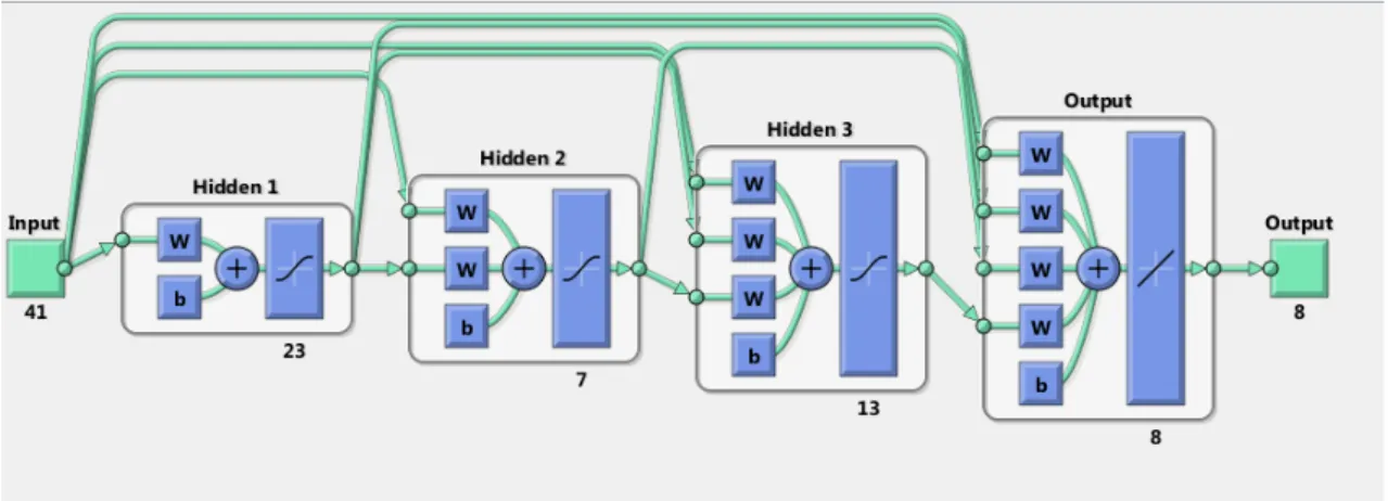
The CFNN network architecture was selected due to the results being noticeably higher than a Pattern recognition or the Fitnet Neural Network architecture. The CFNN is a more complex than the previous mentioned architectures since each layer output is connected with all the others. The constructed CFNN have three hidden layers, 41 inputs one for each feature and eight outputs each output representing one event. The first layer contains 23 neurons and the second layer has seven neurons and on the third layer has 13 neurons. Figure 6 show the size and how the layers and neurons are connected with the other layers and neurons.
Figure 6: Representation of the architecture of Neural Network used to classify the different events
calculates the error of the bias and weights then adjusts the bias and weights using backpropagation. Equation 1 shows the backpropagation used where the Jacobian jX is the performance with respect to the weight and bias variables X and E is all the errors and mu is an adaptive value that increases until the performance value decreases or it reached the max value of mu. When the performance value have decreased or mu reaches maximum value the changes are done on the network and mu value is decreased5. The initial value of mu is set to 0.001 and each increase is a factor of 10 and the decrease is factor of 0.1 and maximum value of mu is 1e10. The performance of the ANN is the Mean Square Error (MSE) of the bias and weights.
jj = jX ∗ jX je = jX ∗ E
dX = −(jj + I ∗ mu)/je
(1)
The training of the ANN will stop if any of the sets criteria is achieved. The set of criteria is maximum amount of epoch, performance value, and validation checks. The epoch maximum is set to 1000 so it ensures that there will not be any infinity loops while training. If the performance value reaches 0 the training will stop since it reached the best performance value from the training data possible. The training is using the validation dataset to protect the network from being overtrained on the training data. When the ANN have passed six validation checks in a row that criterion is achieved, this is the criterion that will have the highest chance of being accomplished first. When any of the criteria is achieved the model of trained ANN is finished. This procedure is repeated five times, one for each set of training and validation data. The model that had the lowest performance value is then chosen to be the final model used to test the network using the test part of the data to get the unbiased results.
5.3
Hidden Markov model
A classifier was implemented using Hidden Markov Model. First, all the required data is loaded and the features are extracted. The features are divided into 8 different matrices, one for every event. The matrices are then rotated appropriately to be compatible with the model.
The implementation is done in MATLAB using a toolbox created by Kevin Murphy called Hidden Markov Model (HMM) Toolbox for MATLAB6. Unlike the HMM toolbox that is provided in
MATLAB that only handles discrete data, this toolbox can handle continuous data using Gaussian outputs. This toolbox is also able to handle mixture of Gaussian outputs.
The model is created by implementing eight different HMMs, one for each event. The models are separately initialized and trained with their corresponding matrix that contains the extracted features. For every model, the amount of Gaussian mixtures and the amount of hidden states can be given. In this experiment, the amount of state is set to 1, 2 or 3 depending on the type of event. The amount of Gaussian mixture is initialized to 2 or 3. The performance of the models will vary depending on the choice of mixtures and states; initializing them to the correct values is essential for an HMM classifier to work properly.
The training is done using an Expectation-maximization algorithm that is known as Baum-Welch algorithm. Initially, the state of the model and the transition matrix is randomly generated. The training data is then fed to the algorithm and the EM algorithm iterates forward and backwards multiple times to recalculate and precise the parameters. This process is done for all the eight different models for their own given data.
Once the training is done for each of the models new sequences of observations are ready to be classified. This process works by providing the sequence of some measured data to each of the models. For every model, the log-likelihood of the sequence matching the model is calculated and the maximum is chosen as follows:
5https://se.mathworks.com/help/nnet/ref/trainlm.html 6
max(L1, L2, . . . , Ln)
where n is the total amount of models (in this case eight since there are eight different events) and where Liis the log-likelihood for a given sequence and a model. When the maximum log-likelihood
is found, the sequence is assumed to belong to that model. This can produce false-positives, so the actual event type is saved and later compared to calculate the precision rates of the models. Figure 7 shows a code snippet of a HMM implemented in MATLAB using the Kevin Murphy’s toolbox. The amount of Gaussian mixtures is set to M = 2 and the amount of states is set to Q = 2. Based on these parameters, some initial matrices are randomly generated. A 2D matrix containing training data is then fed to the model, and the Baum Welch EM algorithm is applied for 10 iterations updating the parameters every time. When the model is done training, another arbitrary long sequence testData, that contains some observables, is provided to the model. The log-likelihood of the sequence belonging to the model is calculated. This value can then for example be compared to another model, and depending on which model produces the highest log-likelihood the unknown sequence of observables will be classified as such.
1 M = 2; % Mixtures
2 Q = 2; % Amount of states
3
4 % Randomly generate start parameters
5 prior0 = normalise(rand(Q,1)); 6 trans0 = mk stochastic(rand(Q,Q));
7 [mul0, sig0 ] = mixgauss init(Q∗M, featRun,’full’) ; 8 mul0 = reshape(mu0, [O Q M]);
9 sig0 = reshape(Sigma0, [O O Q M]); 10 mix0 = mk stochastic(rand(Q,M)); 11
12 % Feed input from data
13 % Train using EM algorithm for 10 iterations to improve parameters
14 [LL, prior1 , transmat1, mul1, sig1, mix1] = ...
15 mhmm em(data, prior0, transmat0, mul0, sig0, mix0, ’max iter’, 10); 16
17 % Calculate the log−likelihood of a new sequence testData
18 % to determine if it belongs to the model
19 loglik = mhmm logprob(testData, prior1, transmat1, mul1, sig1, mix1);
Figure 7: A Hidden Markov Model implementation in MATLAB
Initially, 20% of the data will be reserved for testing. This data is not touched and is not a part of the training phase. The remaining data will be used for a k-fold cross validation where five different models will be trained and compared. In every iteration, the data will be divided into two parts: one part as the training data and the other as validation. 80% of the data is used to train the model, and the remaining 20% is used to validate the model to find the optimal parameters. The best performing model, according to the cross validation, will then be selected as the final model. Once a final model has been selected the training phase is complete and the data that is independent of the training (the test data) is tested and evaluated. This process ensures that the data that is being classified is not in any way already a part of the model and it ensured that the result is not biased.
6
Results
6.1
Overview
Section 6.2 and 6.3 the result of the two different experiments that were conducted will be presented. In section 6.2, one model for an ANN implementation and one model using a HMM implementation will be presented using a fixed window size of 100 sensor readings. In section 6.3 one model for an ANN implementation and one model using a HMM implementation will be presented using an overlapping window size of 100 sensor readings with 25% crossover.
For each model, a test confusion matrix will be presented. The test confusion matrix represents a multiclass classification confusion matrix that essentially describes the performance of the specific model. The confusion matrix shows how well the model managed to classify the different events. More specifically, a confusion matrix compares the predicted classes that the model predicts with the actual classes.
Figure 8 illustrates a confusion matrix example of a three class classification of dogs, cats and birds. As seen in the matrix, it compares the output class (the class that the model has predicted) with the target class (the actual classes). Each row in the matrix shows all the predicted instances of a certain class, while each column shows all the instances of the actual target class that the model should have predicted. This particular model in 8 correctly predicted two out of three dogs, while the third dog was misclassified as a bird. Moreover, the model misclassified one instance of the class cat and one instance of the class bird as the class dog.
Figure 8: Multiclass confusion matrix example
In addition to the confusion matrices, a table for each of the model will be presented containing information of the eight different events. These values are derived from the test confusion matrix and are the following:
• Positive (P), which refers to total amount of positive values (that belongs to the specific event being predicted)
• Negative (N), which refers to the total amount of negative values (that belongs to some other event)
• True Positive (TP), which is the amount of positive values that gets correctly classified as positive
• True Negative (TN), which is the amount of negative values that were correctly classified as negative
• False Negative (FN), which is the amount of positive values that were misclassified as negative • True Positive Rate (TPR) or sensitivity is the probability of the model predicting positive
when the data is positive
• True Negative Rate (TNR) or specificity is the probability of the model predicting negative when the data is negative
• Positive Predictive Value (PPV) shows the probability that the value is positive when it gets classified as positive
• Negative Predictive Value (NPV) shows the probability that the value is negative when it gets classified as negative
• Accuracy (ACC) describes the overall probability that the event will be classified correctly Positive or negative in this case will be the specific type of event that is being analyzed. For example, if the event ”walk” is being analyzed, then a dataset belonging to that event will be positive and all other datasets that belong to another class will be be negative (other). If a walking event were to be misclassified as something else, then that would produce a false negative.
6.2
Experiment 1: Fixed window
This section presents the results of the first experiment using a fixed window size of 100 sensor readings for both of the ANN and HMM implementations.
6.2.1 Artificial Neural Network
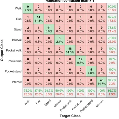
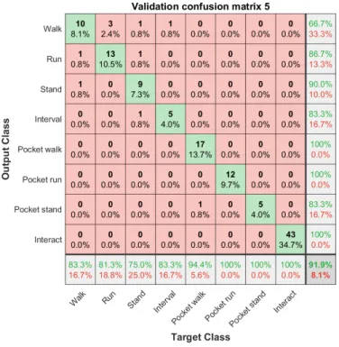
The ANN model with the the lowest performance value (MSE) using the validation dataset as input was selected as final model for the test dataset. The selected model had a performance value of 0.022282 and the average MSE of all the five models was 0.0268338. The other models in the 5-fold validation that was were selected received a performance value of 0.030631, 0.022719, 0.034704 and 0.023833. Appendix A.1 contains the confusion matrices of all five models from the validation phase. The final validation model achieved an overall accuracy of 93.5%, classifying most events with an accuracy of 91.7% or higher. The model underperformed when classify the interval event, however, when the ANN model predicted an event as interval, it predicted the event correctly two out of three times.
Figure 9 represents a confusion matrix showing the achieved results on the final ANN model using the test data as input data in the first experiment using a window size of 100 sensor readings. When the test dataset was classified on the chosen model it got a lower overall accuracy of 90.9% compared to the 93.5% it achieved during training. The ANN model is able to classify most events correctly, a big difference is when classifying standing and running where it standing was classified correctly with only an accuracy of 73.3% and running at 85%. The events pocket walk, pocket run and interact were always classified correctly, and there were no false positives on pocket walk and pocket run.
The values in Table 1 are taken from the test confusion matrix shown in figure 9 to provide a broader look at the model’s performance on test dataset. The accuracy for the different performance metrics are all 94.81% or higher.
Figure 9: ANN confusion matrix on test set with 0% crossover
Walk Run Stand Interval P. walk P. run P. stand Interact
P 14 20 15 8 22 14 7 54 N 140 134 139 146 132 140 147 100 TP 13 17 11 3 22 13 7 54 FP 4 4 1 3 0 0 1 1 TN 136 130 138 143 132 130 136 99 FN 1 3 4 5 0 1 0 0 TPR 92.86% 85.00% 73.33% 37.50% 100.00% 92.86% 100.00% 100.00% TNR 97.14% 97.01% 99.28% 97.95 % 100.00% 100.00% 99.32% 99.00% PPV 76.47% 80.95% 91.67% 50.00% 100.00% 100.00% 87.50% 98.18% NPV 99.27% 97.74% 97.18% 96.62% 100.00% 99.29% 100.00% 100.00% ACC 96.75% 95.45% 96.75% 94.81% 100.00% 99.35% 99.35% 99.35%
Table 1: ANN sensitivity and specificity table with 0% crossover
6.2.2 Hidden Markov Model
During the training phase of the model, a 5-fold validation is done. In appendix B.1 the five different confusion matrices for the validation models can be found. The final model is selected based on how the five different validation models perform. E.g. the model that has the highest accuracy is chosen as the final model.
Figure 10 represents a confusion matrix showing the achieved results for the final HMM model on the test data for experiment 1 using a fixed window size of 100 sensor readings. The model manages to achieve an overall accuracy of 92.9% and is able to correctly classify most of the events. For example, the model manages to correctly classify all of the data for pocket walk, pocket stand and interact. The model is also able to classify the events walk, stand and pocket run with an accuracy higher than 90%. However, the model seems to heavily under perform when trying to classify the interval events, where it only manages to achieve a precision rate of 50%.
Figure 10: HMM confusion matrix on test set with 0% crossover
Table 2. These values are derived from the test confusion matrix shown in figure 10, which provide a broader look at the model’s performance on new test data. The table shows different performance values for each of the eight events. As the table suggests, the model has a sensitivity (TPR) of over 92% for each of the events except run which has a 85% sensitivity and interval which only has a sensitivity of 50%. The specificity (TNR) is consistent across the board, hitting values above 97%. The positive predictive value, negative predictive value and accuracy are all consistently similar as well, where majority of values are above 90% with some values falling down to 80%. As the confusion matrix and table suggests, the model is able to consistently hit an accuracy of over 95% for most of the combinations. Occasionally the algorithm misclassified an event bringing the overall percentage down slightly.
Walk Run Stand Interval P. walk P. run P. stand Interact
P 14 20 15 8 22 14 7 54 N 140 134 139 146 132 140 147 100 TP 13 17 14 4 22 12 7 54 FP 2 4 0 1 1 1 1 1 TN 138 130 139 145 131 139 146 99 FN 1 3 1 4 0 2 0 0 TPR 92.86% 85.00% 93.33% 50.00% 100.00% 100.00% 100.00% 100.00% TNR 98.57% 97.01% 100.00% 99.32% 99.24% 99.24% 99.32% 99.00% PPV 86.67% 80.95% 100.00% 80.00% 95.65% 92.31% 87.50% 98.18% NPV 99.28% 97.74% 99.29% 97.32% 100.00% 100.00% 100.00% 100.00% ACC 98.05% 95.45% 99.35% 96.75% 99.35% 99.31% 99.35% 99.35%
6.3
Experiment 2: Overlapping window
This section presents the results of the second experiment using a sliding window of size 100 sensor readings using 25% crossover on both of the ANN and HMM implementations.
6.3.1 Artificial Neural Network
The ANN model for selected as the final model using 25% crossover dataset was the one with the lowest performance value (MSE) using the validation dataset as input was selected as final model for the test dataset. The selected model’s MSE value was 0.022282 and the average MSE of all the five models was 0.020242. The other four models had MSE values of 0.023089, 0.022460, 0.021584 and 0.017883. The confusion matrices for all models are displayed in Appendix A.2. When comparing the results on the validation phase from experiment 1 and 2, the results show that using a 25% crossover on the window gave a more stable accuracy on the events and less errors during training. The average accuracy gained while classifying the validation dataset was 95.2%, and as shown in the first experiment, it had high misclassification rate on interval where it only achieved an accuracy of 33.3%.
Figure 11 represents the confusion matrix while classifying the test dataset on the chosen ANN model. This model is able to classify the test dataset with an average accuracy of 92.9%. As seen during the training phase, the classification on interval brings down the overall accuracy. Compared to the model from the first experiment this model had a more stable result on walking and standing. However this model had some problems while classifying running and was predicting all events except pocket run and pocket stand. Since it misclassified running seven out of 28 times, it got an accuracy of 75%. This is both lower than the model in the validation phase and the model in experiment 1 which got 90% and 85%, respectively.
Figure 11: ANN confusion matrix on test set with 25% crossover
The values in Table 3 are taken from the test confusion matrix shown in figure 11 to provide a broader look at the model’s performance on test dataset. From this table we can see that the
accuracy on all the events are 96.67% or higher and all event except standing and interval have more than 90% PPV.
Walk Run Stand Interval P. walk P. run P. stand Interact
P 21 28 22 8 30 20 9 72 N 189 182 188 202 180 190 201 138 TP 19 21 21 3 30 20 9 72 FP 2 0 5 2 1 0 1 4 TN 187 182 183 200 179 190 200 134 FN 2 7 1 5 0 0 0 0 TPR 90.48% 75.00% 95.45% 37.50% 100.00% 100.00% 100.00% 100.00% TNR 98.94% 100.00% 97.34% 99.01 % 99.44% 100.00% 99.50% 97.10% PPV 90.48% 100.00% 80.77% 60.00% 96.77% 100.00% 90.00% 94.74% NPV 98.94% 96.30% 99.46% 97.56% 100.00% 100.00% 100.00% 100.00% ACC 98.10% 96.67% 97.14% 96.67% 99.52% 100.00% 99.52% 98.10%
Table 3: ANN sensitivity and specificity table with 25% crossover
6.3.2 Hidden Markov Model
The second experiment that was tested using the HMM implementation was by extracting the features using a sliding window with a 25% crossover. The model in this experiment was trained using cross validation. Five different models were tested in the validation phase and one final model was selected according to the overall accuracy of the models. The confusion matrices for the five validation models can be found in Appendix B.2 fort further viewing.
The results of the final test is shown in the confusion matrix in figure 12. As displayed in the confu-sion matrix, the model manages to reach an accuracy of 93.3% which is a very small improvement on the overall accuracy compared to the model in the previous experiment with a fixed window size. Most significantly, this new model is able to classify the pocket run event with a higher accuracy compared to the previous model. The model seems to perform worse when classifying walking, running and standing but the jump in the pocket run accuracy is greater than the combined loss which results in a slightly higher overall accuracy. Like the previous model in experiment 1, this model seems to be unable to achieve a higher accuracy than 50% when classifying the interval event.
Figure 12: HMM confusion matrix on test set with 25% crossover
The individual values for each of the events are shown in table 4. These values are extracted from the test confusion matrix and show the statistics for each of the events.Even though that the overall accuracy experiment 2 was higher than experiment 1, it is easily noticeable that there are more scenarios in experiment 2 where the probability of certain combinations of measurements fall below 85%. In experiment 1, there were only three scenarios where the accuracy fell below 85%. Here, as seen in the table, there are five different scenarios where the accuracy falls below 85%. Even though the model has a higher overall accuracy than the model in experiment 1, it is achieving that by being less consistent across the the board where the best performing measurements are performing better while the worse performing measurements are worse in comparison.
Walk Run Stand Interval P. walk P. run P. stand Interact
P 21 28 22 8 30 20 9 72 N 189 182 188 202 180 190 201 138 TP 19 22 20 4 30 20 9 72 FP 4 1 0 4 0 0 3 2 TN 185 181 188 198 180 190 198 136 FN 2 6 2 4 0 0 0 0 TPR 90.48% 78.57% 90.91% 50.00% 100.00% 100.00% 100.00% 100.00% TNR 97.88% 99.45% 100.00% 98.02% 100.00% 100.00% 98.51% 98.55% PPV 82.61% 95.65% 100.00% 50.00% 100.00% 100.00% 75.00% 97.30% NPV 98.93% 96.79% 98.95% 98.02% 100.00% 100.00% 100.00% 100.00% ACC 97.14% 96.67% 99.05% 96.19% 100.00% 100.00% 98.57% 99.05%
7
Discussion
One of the motivations for the study of this thesis was to use valuable information that phones already contain and produce and to use it for something practical. In this thesis, a third party application was used to gather data for our models. The reason for this was to access what could be done with information that is already available to us.
The events that are focused on in this thesis were chosen according to previous studies. Some events such as interval and interact were added to widen the scope of the thesis and to contribute with something to the research field. Another decision that was made to contribute to the area was to mix two different phone placements.
Observing previous studies it was clear that the most commonly used algorithms for similar type of research were Artificial Neural Network and Hidden Markov Model. One of the main objectives of this thesis was to find the current state of the art techniques and algorithms in the field. Hence, the two chosen algorithms that were implemented in this thesis were Artificial Neural Network and Hidden Markov Model.
In this study, the window size was based on amount of sensor readings and not elapsed time, unlike other most other studies, such as the study done by Eric Andersson [3] where a window size of 10 seconds was utilized. Due to the third-party application having irregularities in the sampling rate, where each window could wary up to one second, a window size based on a fixed number of sensor readings was used. Approximately, however, a window size in this study was around 7.5 seconds. In another study by Kwapisz et al. [10], a window size of 200 was utilized. While experimenting with the values, before the main implementation was done, it was clear that the classification algorithms performed worse the smaller the window size was. A window size of 100 was chosen because it was sufficiently small enough while still retaining a high enough accuracy.
The table in figure 5 shows an overview of the accuracies for ANN and HMM for the two different experiments that were conducted. Both ANN and HMM seemed to perform quite similarly, hit-ting an overall accuracy higher than 90%. HMM seemed to perform slightly better with a fixed window size, but with a crossover rate of 25% both of the models seemed to hit a similar accuracy rate of approximately 93%. The ANN algorithm seemed get a better performance increase when using sliding window compared to a fixed window size gaining a 2% increase, whereas the HMM implementation only gained an overall accuracy of 0.4%.
Model Experiment 1 Experiment 2
ANN 90.9% 92.9%
HMM 92.9% 93.3%
Table 5: Summary of the accuracies of the final models
The HMM based model in experiment 1 had an overall rating of 92.9% where all of the eight events except interval had a classification accuracy of 85% or more. In experiment 2, the HMM model had a greater overall classification accuracy but with the cost of the running event falling below 80% accuracy. Likewise, looking at individual One vs All classification results, the model in experiment one manages to have a more stable accuracy across the individual events, even though the overall accuracy is slightly lower.
In the ANN-based model in experiment 1, the overall rating was 90.1% where it was able to classify all events with accuracy of 85% or higher. In experiment 2 the ANN had slightly higher overall accuracy than the results in the experiment 1, and it had improvements on classifying most events except running that was classified at 75% or higher. Looking at the One vs all classification results, the second experiment has a higher certainty that the predicted event is the correct one
than experiment one. The number of layers and size of each layer was selected using trial and error testing to find the better size. These tests were done by creating random sized networks and training them to see the accuracy on the validation dataset. The selected size was the test that produced the most stable results during the implementation. However the network could be improved in accuracy or the computational power needed to run the ANN by optimizing the size of the network.
Important to distinct is that even though the overall classification accuracy rate for a model might be high, another model with a lower overall classification rate could be preferable depending on how the individual events are getting classified from between the models. For example, if the classification of a certain event is more valuable than another, then one would prefer a model having a higher classification rate on that event even though the overall accuracy may be lower. For pedestrians in particular, events that are risky in their nature might be of priority. This means that events that potentially could be a risk to the public (such as suddenly stopping or running) should be prioritized if the intention is to identify and warn others of risky behaviors. Depending on the end goal of the model, an appropriate performance metric should be taken into account. Seliya et al. [27] discuss the relationships of different performance metrics for classifiers. In the study they compare 22 different metrics and evaluate their imbalances.
Since the interval event is created by altering between the events standing and stopping, it gave similar values on the features as the standing and running event. This is seen in the results, where interval was mostly misclassified as standing or running. Another problem with interval was during collection of the data for this event, each sample had too many irregularities in timings since it takes time to stop running. Due to this, there was little point in collecting more data on interval, which is reason as to why it only consists of 3.8% of the total sampled data. However, this event still affects the results on the other events such as standing and running.
As shown in both of the models, the pocket type events and interact were classified with a sig-nificantly higher accuracy than the other events. This is most likely due to the fact that these events in particular were added as events later on and not all the subjects from the previous events’ dataset was in this dataset. Furthermore, a larger amount of data was collected for these events than the other events that had a lower accuracy. A third contributing factor was that the subjects of the pocket type events and interact were overall more similar physically compared to the other events.
In this study, phone placement was taken into consideration when classifying the behavior of a pedestrian (e.g. there were two events for walking, one with the phone on the arm and one in the pocket). These two events could arguably be merged into one event where the model is trained using data where the phone is placed in both places as the event itself is what is important to identify. One of the reason as to why this distinction was made was to determine if a machine learning model even could separate the two. As seen in this study, the model clearly manages to separate the two quite well so merging multiple phone placements into one event could be something to investigate further in the future.
7.1
Limitations
Road transportation is a complex system with a lot of varying variables and events. In order to model such a system one has to break it down to smaller sub models. In this thesis, the goal was to investigate and analyze the behavior of a pedestrian. More specifically, eight different finite events for a pedestrian were chosen and used for the classification models. The results presented in this study are thereby limited to these eight specific events. Using either fewer, more or another set of events would change the classification accuracies of the models.
Another limitation of this study was the amount of subjects that were used to gather the data for our models. In total, five subjects were used to collect the data. Using more subjects could lower the classification accuracy of the models depending on the differences between the subjects. The reason for this being that the data collected varies from subject to subject, and the more physical differences there are between the subjects, the more the data will vary. The model is also limited
to the subjects that it previously has trained on. In other words, if new data for a new subject, that the model previously has not seen, is inputted to the models then the models would almost certainly not perform as well.
The goal of this study was to investigate how machine learning models could be implemented using data from IMU sensors and GPS. A conscious decision was made to not store any information of the subjects that were used to gather the data. Confidential data of the subject such as gender, weight, height or other physical parameters can be used as a separate feature for the models and it would likely improve the overall accuracies of the models. This is arguably more important the more subjects you have, especially when the different physical parameters of the subjects vary a lot. Due to confidential reasons and because of our main objective of this thesis, these parameters were not considered.
The sensor readings for the subjects were collected from some predefined set of areas. Thus, the presented results in this thesis are limited to these set of areas since collection of data in other areas are likely to slightly differ. For the models, a set amount of features was used. These features were defined before the models were implemented. Using different sets of features would affect the overall classification accuracy of the models. Likewise, if another window size other than 100 or a different crossover rate than 25% were to be used, it would most likely affect the results as well.
8
Conclusions
The aim of this thesis was to investigate and analyze the behaviors of a pedestrian in road transport using machine learning. More concretely, the goal was to investigate which features could be extracted from IMU sensors and GPS signals to model different events of a pedestrian and to find out which events of a pedestrian that can be classified using these features. Furthermore, the aim was to research how such a model can be implemented and which machine learning algorithms are relevant in terms of classification accuracy.
In this thesis, eight different types of events were focused on. These events conclude walking, standing and running with the phone mounted on the arm, walking standing and running with the phone in the pocket and lastly an interactive event with the phone in the hand of the subject. The IMU sensor and the GPS in the phone were utilized to collect data. From the sensor readings, a set of features were extracted based on previous studies. These features were average acceleration, standard deviation, average absolute difference, average resultant acceleration, average speed and a custom bin collection.
In total, four different models were implemented and presented using two different machine learning algorithms: Artificial Neural Network and Hidden Markov Model. The choice of machine learning algorithms was based on previous studies done in the field, where ANN and HMM were the two most frequently used algorithms that showed promising results.
For both ANN and HMM, two different experiments were conducted. In the first experiment, the features were extracted with a fixed window size of 100 sensor readings per window. In the second experiment, the window size remained the same but a sliding window with 25% crossover rate was utilized instead of a fixed window. The proposed models in this study managed to achieve an accuracy of approximately 93% where HMM performed slightly better, especially in the first experiment. The ANN model seemed to gain a greater performance increase in terms of classification accuracy when switching from a fixed window size to a sliding window, gaining a 2% accuracy increase.
Other than the interval event which had an classification accuracy of approximately 50%, the models managed to maintain high classification accuracy across all the events. The most probable reason as to why the interval event did not perform so well is because the event in itself consists of walking and running so the interval event got mistakenly classified as either running or walking multiple times.
The proposed models in this study showed promising results. Real time classification applications will without a doubt be able to be implemented in the future. Currently, however, there is still room for research in the field. More specifically, being able to model real risky behaviors of a pedestrian, such as suddenly running or suddenly stopping, is important.
9
Future Work
Even though the presented models showed promising results, there are still opportunities for en-hancement. In order to make the algorithms more robust, there is a need for a larger amount of training data preferably with a bigger variance on the subjects attributes, e.g. height, length and weight. Looking at the presented results in this study, it can be seen that the events that had fewer subjects and more data overall, received a higher and better results than the ones with more subjects and less data.
As stated in the discussion, in this thesis, sensitive data such as gender, weight and height of the subjects were not taken into account as apart the model. Studies in the future could be conducted were such information is taken into consideration. Information that are specific and unique to a single subject is most likely very important, especially when many subjects are used with varied information. This of course raises some privacy concerns, especially when speculating about real time applications and would require consent from the user. Even though such study would require the researchers to tackle some ethical concerns, the potential information that such study can provide is very valuable to the field.
The results from ANN is overall decent but it can be optimized using algorithms such as Genetic Algorithms or Differential evolution to find a better size for network by adjusting the amount of layers and size on each layer.
The validation of the HMM is done by looking at the overall accuracy of the different folds. This validation step could be improved by using a more robust and efficient validation technique. Furthermore, the HMM can be altered quite significantly by changing the different parameters (such as amount of states and mixtures) which could affect the overall accuracy positively. In order to build more refined and accurate models, a more reliable and faster way of sampling the data from a smartphone is needed. Receiving the sampled data at a faster rate and more accurately, would ensure a more efficient model. By increasing the amount of samples, the physical time of the window size could be decreased making it closer to real-time.
On a broader scale, for this type of classification to be able to identify potential risky behaviors of pedestrian, additional events have to be investigated. In particular, risky events out of the ordinary that could potentially cause an accident, such as suddenly stopping or suddenly running.