BACHELOR THESIS WITHIN: Economics NUMBER OF CREDITS: 15hp
PROGRAMME OF STUDY: International Economics
and Policy
AUTHOR: Ademir Cabaravdic & Martin Nilsson JÖNKÖPING May 2017
The Effect of Corruption
on Economic Growth
Does corruption show a significance effect in the growth
of an economy?
Bachelor Thesis in Economics
Title: The Effect of Corruption on Economic Growth
Does corruption show a significant effect in the growth of an economy? Authors: Ademir Cabaravdic & Martin Nilsson
Tutors: Kristofer Månsson & Mark Bagley
Date: 2017-05-22
Subject terms: Corruption, Economic Growth, GDP, FDI
Abstract
Corruption as a subject of economic research is a trending topic, and in the age of technology when one has access to more information, bribes and corrupted actions are more easily detected. This thesis tries to answer the question “Does corruption show a significant effect in the growth of an economy” in the case of Southern Europe. The method used to examine this relationship is linear panel data regression model with robust standard errors specified in Methodology section. The outcomes of three different regressions with fixed effects are presented in section Results implying that corruption has a positive effect on real gross domestic product per capita growth of the countries in question. This means that in the short-run, corruption may have positive effect on economic growth in Southern Europe. Such an outcome provides evidence and confirms the hypothesis that corruption can grease the wheels of an economy by avoiding inefficient bureaucracy.
Acknowledgements
We would like to express our sincere gratitude to the people at Jönköping International Business School that have participated in our journey of finalizing this Bachelor Thesis.
Foremost we want to thank our supervisors who have advised and supported us throughout the entire process.
We would also like to show our appreciation to our family and friends who have supported us in with our study.
Table of Contents
1
Introduction ... 1
1.1 Background ... 1
1.2 Previous studies ... 1
1.3 Purpose and Contribution ... 3
1.4 Limitations ... 3
2
Theory ... 4
2.1 The Sanders and the Greasers ... 4
3
Data ... 6
3.1 Sample ... 6 3.2 Variables ... 7 3.2.1 Dependent Variable ... 8 3.2.2 Independent Variables ... 94
Methodology ... 12
5
Results ... 14
7
Discussion ... 18
8
Conclusion ... 20
References ... 21
Figures Figure 4-1 Model 1 and 2 ... 13Figure 4-2 Model 3 ... 14
Figure 0-1 Chi-Square test Hausman ... 24
Tables Table 3-1 List of variables ... 8
Table 3-2 Descriptive Statistics ... 11
Table 5-1 Hausman Test Coefficients ... 15
Table 5-2 Notes to table 5-2. Linear regression panel data model with fixed effects and robust standard errors. ... 16
Table 0-1 Autocorrelation test ... 23
Table 0-2 Correlation table ... 23
Table 0-3 Hausman Test ... 24
Appendix
9 Appendix 1 ... 231 Introduction
1.1 Background
”Dishonest or fraudulent conduct by those in power, typically involving bribery” reads the Oxford dictionary’s definition of corruption. Although corruption may take many forms, it is most often for personal gain through the use of entrusted power (Aidt, 2009; Mauro, 1995). According to Levy (2007) there has been a long debate on the impacts of corruption, however the absence of hard quantitative data, most likely because of its illegal nature, has complicated the corruption-related debates. Transparency International publishes the corruption index, which is widely used for economic research. It is an index of perceived corruption based on petty, grand and public corruption; it will be further described in the data section. The general thought of corruption and economic growth divides economists into two camps. The most common idea supported and presented by economists such as Murphy, K. M., Shleifer, A., & Vishny, R. W. (1993) and Mauro (1995) is that corruption is an obstruction on economic growth and development. That corruption “sands the wheels” of growth; economists supporting this idea are also knows as “sanders”. On the other hand there are economists who believe that corruption could “grease” the wheel of commerce and contribute to steady growth. Leff (1964) and Huntington (1968) propose a theory with the idea that economic growth could be positively affected if individuals could avoid any bureaucratic delays. They also brought forward the idea that employees of the government would be motivated to work harder with the possibility to receive bribes. Economists’ with opinions of this kind will further be referred as “greasers”.
1.2 Previous studies
In this study, a model with panel data regressions is applied, instead of the cross-country regression data models used by Aidt (2009), Mauro (1996) and Barro (1991). The model used in this study will be testing the hypothesis on a new region, which is Southern Europe and the Balkan countries. Furthermore the variable Foreign Direct Investment [FDI] has been added since it is considered as a good indicator of economic growth. Aidt (2004) uses GDP per capita growth rate as a dependent variable when testing his hypothesis, whether perceived corruption has a significant effect on economic growth. His study is performed on 60-80 developed and developing countries and it did not include Eastern Europe or any states of
the former Soviet Union. This study is conducted on countries in Southern Europe and the Balkan region for any significant impact corruption has on economic growth or on investment. The interesting point to emphasize is that both Aidt (2009) and Mauro (1996) are using a significantly larger quantity of countries in their models, however they are testing the effect corruption has on economic growth and development on average data over a period of time for all of their variables, while this study is creating a model that measures actual value of the country for each variable and for each year.
Since there are no proper statistics of corruption, economists use indices to compile tests of corruption with different variables. Transparency International began in 1996 to, every year, present a Corruption Perception Index (CPI). This index is determined by expert assessments and opinion surveys, based on thirteen surveys from twelve different institutions. Furthermore, CPI is based on perceived corruption, rather than absolute numbers of corruption. Since this study is compiled by data received from CPI, everything presented in this study is based on perceived corruption.
Transparency International (2016) has recently released a study, which shows that the public
perception of corruption is a major problem especially in the Balkan countries. One in three citizens believe that corruption is one of the main problems facing their country. The article (Transparency International, 2016) also states that 53 percent of the individuals that answered their questionnaire thought that their government was doing a poor job of fighting corruption in the public sector. The study showed worrying numbers of people’s perception on corruption, and 30 percent of the people were hesitant to even report corruption due to fear of consequences. This paper will review the different perspectives of corruption, and an empirical study, of 14 Southern European and Balkan countries over a twelve-year period will be conducted and presented.
The 14 countries included in this study are Albania, Bulgaria, Croatia, Cyprus, Greece, Italy, Macedonia (FYR), Montenegro, Portugal, Romania, Serbia, Spain and Turkey. Some of the countries have been excluded due to insufficient data.
1.3 Purpose and Contribution
The purpose of this study is to test the hypothesis whether perceived corruption has a significant effect on economic growth as measured in real gross domestic product per capita growth.
The close relationship between corruption and the economic performance of countries have been subjected to numerous studies (Leff, 1964; Huntington, 1968; Aidt, 2009; Levy, 2007; Mauro, 2002; Barro, 2013). Does corruption have short-term effects on the economy? If so, this research will examine if these short-term effects act like sand or grease for the growth of economy.
The contribution to the topic is to present results whether corruption in Southern European and Balkan countries has negative or positive effects on economic growth. Panel regression models have been constructed on cross-national data from countries in Southern Europe and Balkan countries. Previous studies present results of the effect corruption has on economic growth for different regions of the world, such as America (Barro, 1991), Europe (Aidt, 2009) and Asia (Khan, 2000). However no relevant previous studies have been found on the geographical area chosen for this thesis.
All the results and values of this research are presented in order to agree with the ‘‘sanders” or the ‘‘greasers” of previous economists researches of corruption and economic growth. Results on Southern Europe and the Balkan countries are presented to see how corruption affects economic growth in these countries and in a way our contribution is made to this topic by broaden the scope of studies, which can help in understanding this phenomenon.
1.4 Limitations
Many researchers have tried to gather evidence on the relationship between economic growth and corruption. However, it is believed that a large obstacle for empirical research on corruption is that the only indications of corruption that exist are perceived corruption indices. Transparency International is an organization on the topic of measuring corruption; however it is still an index based on the perception of experts and randomly selected individuals. Economists often use these indicators for empirical research. Even though CPI is a good indicator since it measures the level of corruption in the public sector of a country, it still has some disadvantages. CPI is based on citizens’ opinions, which can also represent
lagged perception of corruption in the country. This simply implies that level of corruption in the index for a specific year is actually the represented level of corruption from the perceived corruption of the previous of years. However, since there is no real evidence for this, we use the current years as a measure of the corruption. One other issue with CPI is the subjectivity. Since the index is based on humans’ perceptions, it represents the level of corruption, which is recognized by citizens of the countries. This causes CPI not to capture all corruption in the system of one country and therefore it affects the results by providing incomplete data. On the other side, Transparency International has been computing this index for many years, and it is as mentioned before, used in other similar studies, investigating corruption and economics growth relationship in countries. Articles on whether these indices1 are accurate enough have emerged lately and Campbell’s (2013) article Perception is not Reality is one of the most recent and relevant articles on the subject.
2 Theory
2.1 The Sanders and the Greasers
Aidt (2009) states that corruption and its effect on economic growth is populated by two types of supporters, or as he expresses it ‘‘Two different views on corruption”. Aidt (2009) further defines one side as “greasers”; whom are economists who believe that if corruption is contributed efficiently it could “grease the wheels of commerce”. One of the founding researchers who paved the way for this idea was Leff (1964): he wrote an article in 1964 and his work gave way to the first theoretical framework of the ‘‘greasing” aspect on the topic. Leff (1964) showed that under certain circumstances corruption could have a positive effect on economic growth and/or investments. His essential thought was that through corruption, a country could make beneficial trades that might not have happened unless corruption was a part of the equation. To illustrate his argument and further clarify his theory, he gave an example on how corruption could contribute positively with Chilean and Brazilian price control regulation in the 1960s. During this period, officials in Brazilian and Chilean
1 The leading indexes are: CPI (Corruption Perception Index provided by Transparency International)
CC(control of corruption provided by Worldwide Governance Indicator, a project at World Bank) ICRG(International Country Risk Guide, provided by a private business consulting company)
governments enforced the bureaucracy to make price regulations on food (freezing the prices) in order to keep the stagnated inflation under control. In Chile the public acted loyally towards the regulation and prices stayed relatively stagnated. Inflation started to rise but at the cost of a decrease in food production. In Brazil however, the bureaucracy could not hinder sabotage from the public on the presented price regulations and an increase in prices followed, the production of food however increased as well as it partially stabilized the course of inflation. His opinion of the effects of corruption was described as the success of entrepreneurs and corrupt officials producing a more effective policy than the government. Another example of corruption acting as grease to the wheel of commerce is “the Asian paradox”. Asian countries have been known to have a rapid growth for the past decades even though they place high on the perceived corruptions index. “The Asian Paradox” described by Rock and Bennett (2004) as the combination of high corruption and high growth – in terms of stable and mutually beneficial exchanges of government promotional privilege for bribes and kickbacks. Rock and Bennett performed a statistical analysis for five large Asian developing countries, testing for any impact corruption might have on investment and growth. Their results corroborated with the Asian Paradox theory. There is however no explanation as to why this phenomenon exists. Economists have tried to explain the phenomenon by combining characteristics of corruption from earlier empirical investigations (Rock & Bennet, 2004; Ugur & Dasgupta, 2011). According to the paper on corruption and economic growth by the OECD2(2013), there have been a number of possible arguments as to the causes of the paradox, any robust and direct explanation is however yet to be found. Further, Aidt (2009) describes the other side of researchers as “sanders”. The group consists of economists who performed studies with the “sand in the wheels” hypothesis. De Soto (1990) performed an experiment in Peru: he had a theory that too much of Peru’s wealth and economic transactions were performed outside of the official economy. In his attempt to find a reason, he asked fellow researchers to legally set up a factory including two sewing machines. The process took 300 days, working 6 hours a day to get all of the legal documents in order so set up the business. According to the article, it was no longer a question as to why entrepreneurs would try to enter the market with the help of a bribe to speed up the process, or simply stay outside the informal market. In 2002 Simeon Djankov and his fellow
2 An investigation by OECD presented to the G20 leaders at the St. Petersburg summit in September 2013 with the core objective to increase the efforts to fight corruption.
researchers made an empirical study on the regulation of entry of start-up firm in 85 countries to test De Soto’s theory (Djankov et al. 2002). Their study confirmed that countries with heavy regulations for start-up firms were in fact infected with high-perceived corruption and a larger illegal economic sector. According to Mauro’s (2002) article, he states that in recent years researchers recognition of corruption by public officials and other corrupt governance that have a negative effect on economic growth have increased substantially. In his article (Mauro, 2002) he questions why countries do not strive harder to improve their fight against corruption. One of his conclusions on why corruption is so difficult to fight is because in some countries corruption is too widespread for individuals to even try, even though everyone would be better off with the elimination of corruption. He presents two models complementary to each other since they view corruption through two different angles. The first model he displays is the multiple equilibrium in corruption and growth-model, a result he claims not been obtained in modern day research. A basic interpretation is that individuals have to allocate their time between stealing from government expenditures and being productive with any work activity. He compares it with Murphy’s model (Murphy et. al, 1993), where if there are a lot of people stealing then the chances of one getting caught is slim. The second model presented is to test corruption through political instability, where he questions if it could be reinforcement towards economic growth.
3 Data
3.1 Sample
The sample of this study is 14 countries in the Southern European and the Balkan region. This specific area is chosen based on the fact that they have not been the basis or measure of similar studies before. Therefore we have chosen this sample to include a part of the world that had not been researched a lot in terms of corruption and economic growth. Since there are many definitions of Southern Europe, which are based on different metrics, we decide to define Southern Europe as Europe’s three peninsulas, Iberian Peninsula, Apennine Peninsula, and Balkan Peninsula. Those three peninsulas consist of 21 countries, which are used in the models initially. However, due to missing data for Andorra, Gibraltar, San Marino, Vatican, Malta, Kosovo, and Bosnia and Herzegovina, we have to deduct these countries, and the models are eventually constructed with 14 countries for which we could find all values for each variable.
The time span is dictated by two factors. The first factor is relevant data, and trying to collect the latest data available in order for the analysis to provide the most recent and updated results possible. The second dictating factor is the availability of data for the countries in question. Only data for period 2003-2014 could be gathered. This is mainly because numerous countries included in the sample are missing values for either GDP Per Capita Growth or Foreign Direct Investment Net Inflow. Because of these constraints in sampling the data, it comes out to be a strongly balanced panel data for 14 countries with the time span of 12 years. It is also important to note that values for Montenegro between 2003 and 2006 are not used since it was part of Serbia and Montenegro until middle of 2006. To account for this problem, a structural break dummy is constructed for the regressions.
3.2 Variables
Based on previous studies and research (Barro, 2013; Barro, 1991; Aidt, 2009.), the following variables are included in this study. As the dependent variable, we chose the annual growth of real gross domestic product per capita in percentage. This variable is mostly used as an indicator of economic growth in countries (Barro, 1991). As independent variables, we chose Corruption Perception Index, population growth, trade openness as a percentage of gross domestic product, gross fixed capital formation as a percentage of gross domestic product, foreign direct investment net inflow as a percentage of gross domestic product, lagged real gross domestic product per capita growth and finally as mentioned in the previous section a structural break dummy to account for Serbia and Montenegro. All the variables are calculated and gathered on an annual basis starting from 2003 leading up to 2014.
Variable Name Corruption Perception Index Real GDP Per Capita Growth Gross Fixed Capital Formation
Trade Openness Population Growth
FDI Net Inflow Structural Break Dummy Lagged Real GDP Per Capita Growth
Table 3-1 List of variables
3.2.1 Dependent Variable
Real Gross Domestic Product Per capita Growth
The variable that is dependent in this study is real gross domestic product per capita growth expressed in percentages. Since we are trying to estimate the effect of corruption on economic growth, real GDP per capita growth is the most suitable variable to use according to previous researchers such as Toke (2009). Real GDP per capita growth is gathered from World Bank (2017). It is calculated in terms of constant US dollars from 20103. This variable shows real economic growth of countries and provides a good estimation of country’s economic well-being which can be seen from the usage of this indicator. Other studies (Barro, 1991; King & Levine, 1993; Mo, 2001) use this variable to see the economic growth of the countries in their research.
3 It is simply calculated as real GDP per capita in current year t minus real GDP per capita in t-1 and divided
3.2.2 Independent Variables
Corruption Perception Index
Transparency International created Corruption Perception Index [CPI] with the goal to measure
the corruption in public sector of the country. This is a composite index, which represents combination of different indices and surveys and is widely recognized as one of the best measures of corruption. It has been used in other reputable studies (Aidt, 2009), where the effect of corruption on economic growth is examined in a similar manner to our study. CPI is measured on a scale from 0 to 100 where 0 represents maximum perceived corruption and 100 represents country without any perceived corruption. No country is believed to be completely free from at least some amount of public sector corruption. In 2016, the number of countries where CPI was computed was 176 and no country achieved 100 on the scale. This shows the importance of corruption in our study since every part of the world and every nation are familiar with this issue.
Gross Fixed Capital Formation
Gross Fixed Capital Formation [GFCF] is collected from World Bank (2017). It shows “how much of the new value in the economy is invested rather than consumed” (World Bank, 2017). The Gross Fixed Capital Formation variable is measured as a percentage of gross domestic product. Some other studies (Aidt, 2009) use initial investment share instead of gross fixed capital formation as an independent variable, but we could not find all the values for the countries in question and we wanted to be consistent so we chose Gross Fixed Capital Formation variable from World Bank.
Trade Openness
Trade Openness is measured as a share of gross domestic product consisting of the sum of imports and exports of goods and services. It is collected form World Bank (2017). It can take on values higher than 100 percent since it represents summed value of imports and exports instead of netted which is part of a country’s GDP. It is argued (Grossman & Helpman, 1990) that the more open economy is, the more developed it is.
Foreign Direct Investment Net Inflow
From World Bank (2017), one more variable has been retrieved, which is Foreign Direct Investment Net Inflow. This variable represents “share of FDI net inflows of investment to acquire a lasting management interest in an enterprise operating in an economy other than that of the investor” (World Bank, 2017). It is represented as a share of GDP of the country and it may take on the values from 0 to 100 percent.
Population Growth
Furthermore, population growth is collected from the World Bank (2017) database, which represents annual growth in percentage of a country’s population4. This variable may take on any positive or negative percentage value depending on the increase or the decrease of the population.
Structural Break Dummy
This panel study covers 14 countries during the timeframe 2003 to 2014, where two of the countries once were merged. Hence, there is a need to control for some structural breaks. Fortunately, the data in this study already accounts for Kosovo as having separate values from Serbia under this period5, but it is necessary to control for Serbia and Montenegro, as they were one country in parts of this study and in parts of the retrieved data6. Therefore, a structural break dummy which accounts for this problem is created. This leads to a decrease from 168 observations to 164.
4 Population is based on the de facto definition of population (World Bank, 2017).
5 Kosovo and Serbia were one country until February 2008 then the split into separate countries.
Variable No. of
Observations Mean Deviation Standard Min. Max. Real GDP Per Capita Growth 164 1.824 3.935 -8.998 10.505 Corruption Perception Index 164 45.317 12.683 23 71 Gross Fixed Capital Formation 164 23.171 5.370 11.590 40.473
Trade Openness 164 82.458 25.999 45.609 145.328
Population Growth 164 .183 .745 -1.666 1.851
FDI Net Inflow 164 6.067 17.119 -43.462 198.305
Structural Break Dummy 164 .024 .155 0 1
Table 3-2 Descriptive Statistics
Lagged Real Gross Domestic Product Per capita Growth
This is the same variable as Real Gross Domestic Product per Capita, but with a lag of one year which means that for example, the value for 2005 is real GDP per capita growth from 2004. It is used since it is a good estimator of economic growth in this case.
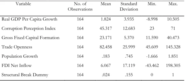
As mentioned in previous section (Table 3-2), the number of observations conducted in this study is 164, reduced from the initial 168 observations due to a structural break dummy for Serbia and Montenegro. Since the countries used in this panel study are mostly developing countries, it is shown that real GDP per capita growth has a maximum of 10.50 percent, but also a minimum of negative 8.99 percent rate of growth. This can potentially be explained by the fact that the period 2003-2014 covers a period of recession, which all countries in this study experienced around 2008. When investigating the CPI variable, the minimum value in this study is 23, which belongs to Serbia and Macedonia in 2003. This is because ex-Yugoslavian countries went through a hard period7 of their history and the effect of war and low growth made people insecure and not as trusting towards their respective governments. On the other hand, Spain scored a maximum value of 71 out of 100 in 2004, however they did as well decline with more than ten points until the year 2014. This exemplifies that the countries in this study still provide great variety due to cultural, national and economical differences, even though they are close to each other geographically.
7 Ex-Yugoslavian countries had a stormy part in their histories and went through demonstrations, war and war
Another explanatory variable that is examined is the population growth variable. Even though it might take on any value, it still stays in the range between negative 1.66 percent and positive 1.85 percent growth. This may not look like a huge difference, however when a country of 5 million inhabitants increases in population more than one percent, it makes huge difference in rough numbers.
4 Methodology
Since economists have different opinions whether corruption greases the wheels of commerce (Leff, 1964; Huntington, 1968) or sands them (Mauro, 1995; Murphy et al., 1993; Toke, 2009) by slowing or even stopping the economic growth of a country, the research done in this paper tries to contribute to this question. The researchers on both sides share arguments for and arguments against their opinions. However since this is a complex issue, this paper hopes to solve, or at least contribute to a better understanding of the subject. As discussed in the data section, six explanatory variables are used together with one structural break dummy, whereof the dummy variable accounts for Montenegro not existing as an independent country before 2006. Using the panel regression study was the best option based on the available observations for the region in question since cross-sectional study covers fewer observations, and time series studies have some gaps in data availability throughout the years. Therefore, the variables gathered from year 2003 until 2014 provide one with all values and allow for strongly balanced panel data. The hypothesis which is being tested in this thesis, by running a panel study on 14 countries under the timeframe from 2003 to 2014, is to observe whether corruption affects economic growth of countries in Southern Europe and Balkan countries and if so, which kind of effect does it have.
Even though previous papers within the field of corruption (Toke, 2009; Barro, 1991; Mauro, 1996), often approach this question by doing cross a-sectional study that is not the course of this paper. Instead, the models in this paper are adjusted for panel data. To test our hypothesis, three linear regression panel data models with fixed effects are specified. All three models that are specified (Model 1; Model 2; Model 3), test for effect of corruption on economic growth. Panel study is chosen since it enables following dynamic changes in both cross-sectional and time series, but also it examines the short-run effects, which are interesting to test for.
When panel study is compiled, one can choose between fixed and random effects to get the regressions which are most appropriate for the study. Both regressions with random and fixed effects have been performed. Based on the results, it is possible to run Hausman test to determine which effects are more appropriate for the regressions in this study. Hausman test makes it possible to determine whether differences between countries are caused by random variances or not, for each country. In this way, Hausman test implies which of these two effects are more appropriate for the regressions (See Figure 0-1 in Appendix 1).
Besides discussion about effects, test for pure autocorrelation is made (See Table 0-1 in Appendix 1). Since results of the test show that there is in fact pure autocorrelation in the data, robust standard errors are used.
Real GDP Per Capita Growthit=β0i+β1*Corruption Perception Index+β2*Lagged Real GDP Per Capita
Growth+β3*Structural Break Dummy+uit (Model 1)
Real GDP Per Capita Growthit=β0i+β1*Corruption Perception Index+β2*Gross Fixed Capital
Formation+β3*Trade Openness+β4*Population Growth+β5*Lagged Real GDP Per Capita
Growth+β6*Structural Break Dummy+uit (Model 2)
Figure 4-1 Model 1 and 2
Correlation matrix (See Table 0-2 in Appendix 1) is also computed in order to check for within-panel correlation structure. None of the variables exceed 0.570 correlation, which is correlation between Gross Fixed Capital Formation and Lagged Real GDP/Capita Growth. These results imply that all of the variables can be used when running linear regression panel models. In further sections, models consist of two simplified versions (Model1; Model 2) where potential different outcomes are going to be tested for. The first variation (Model 1) that is going to be tested is whether CPI, representing corruption in this study, regressed together with lagged real gross domestic product per capita growth affect the real gross domestic product per capita growth, without including the rest of the variables in the regression. In the second variation of the regression (Model 2), all variables except for foreign direct investment net inflow, as a percentage of GDP, are used.
Real GDP Per Capita Growthit=β0i+β1*Corruption Perception Index+β2*Gross Fixed Capital
Formation+β3*Trade Openness+β4*Population Growth+β5*Lagged Real GDP Per Capita Growth+β6*FDI
Net Inflow+β7*Structural Break Dummy+uit (Model 3)
Figure 4-2 Model 3
In all three models (Model 1; Model 2; Model 3), the null hypothesis is that there is no effect of perceived corruption (CPI) in public sector on economic growth. In the section Results, outcomes of the regressions will be examined to see if the null hypothesis is to be accepted or rejected. Based on that, it is possible to estimate the effect of corruption on economic growth in the case of the Southern European countries8.
5 Results
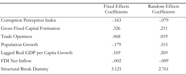
After gathering all the needed variables and choosing the right methodology, three linear regressions are run. Since panel study is done and the area of Southern Europe consists of the countries which are culturally and geographically close to each other, but also, politically and systematically different from one another, fixed effects regressions are used for testing. To control for this and to be sure that fixed effects fit better than random effects, Hausman test is performed. Since the outcome of Hausman test (Figure 0-1 Hausman) is not statistically significant, which means it is below 0.05, the null hypothesis is rejected. This means that differences in coefficients are systematic which implies that fixed effects should be used when running linear regression panel models.
Table Hausman Hausman test Fixed Effects
Coefficients Random Effects Coefficients
Corruption Perception Index -.163 -.079
Gross Fixed Capital Formation .326 .211
Trade Openness .068 .019
Population Growth -.179 .315
Lagged Real GDP per Capita Growth .169 .269
FDI Net Inflow -.002 -.009
Structural Break Dummy 3.121 2.761
Table 5-1 Hausman Test Coefficients
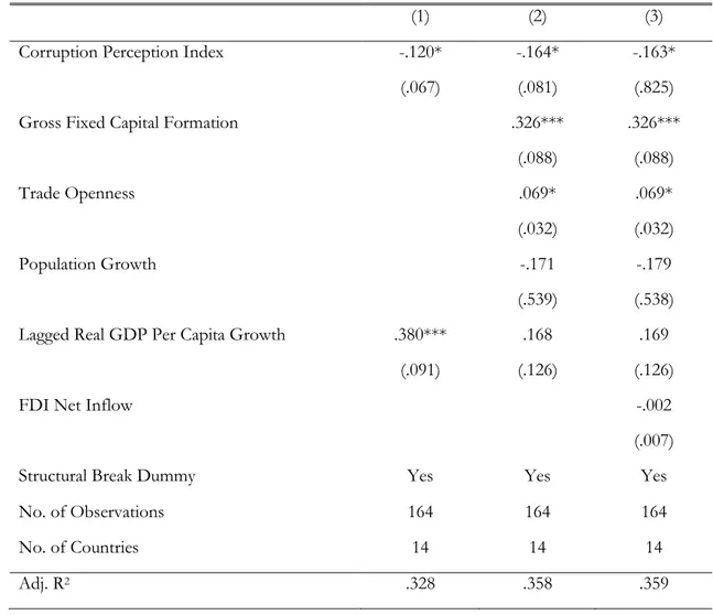
The first regression (1) includes CPI and Lagged Real GDP Per Capita growth in order to see the effect of corruption on economic growth in the Southern European region. Result of this regression is that CPI is statistically significant variable at 10 percent. This regression (1) tests for a clear effect of corruption on economic growth since CPI and Lagged Real GDP Per Capita Growth are included only. Regression (1) implies that increase in CPI by one unit, which means that level of corruption in the countries decreases9, leads to a decrease in economic growth of the country (Real GDP Per Capita Growth) by 0.120 percent. This finding goes hand in hand with claims (Leff, 1964; Huntington 1968) that corruption serves as a greaser of the wheels of the economy. In regression (2), Gross Fixed Capital Formation, Trade Openness and Population Growth are included to see whether the significance and the effect of CPI on economic growth will change. It turned out not to be the case since CPI is still statistically significant at 10 percent with coefficient being negative and even increasing the negative effect on economic growth. This result indicates that one unit decrease in corruption would lead to a decrease in economic growth of the countries by 0.164 percent. Beside this effect, we can see that by including the three new variables in the regression (2), its R-squared increases from 0.328 to 0.358 which implies that the three extra variables explain more of the variation in dependent variable which is economic growth in the case of this study.
Dependent variable: Real GDP Per Capita Growth
(1) (2) (3)
Corruption Perception Index -.120* -.164* -.163*
(.067) (.081) (.825)
Gross Fixed Capital Formation .326*** .326***
(.088) (.088)
Trade Openness .069* .069*
(.032) (.032)
Population Growth -.171 -.179
(.539) (.538) Lagged Real GDP Per Capita Growth .380*** .168 .169
(.091) (.126) (.126)
FDI Net Inflow -.002
(.007)
Structural Break Dummy Yes Yes Yes
No. of Observations 164 164 164
No. of Countries 14 14 14
Adj. R2 .328 .358 .359
Table 5-2 Notes to table 5-2. Linear regression panel data model with fixed effects and robust
standard errors estimates effects of corruption in public sector on economic growth; Robust standard errors are in parentheses’; * significant at 10%, **significant at 5%, ***significant at 1%.
Trade Openness and Gross Fixed Capital Formation are good indicators of economic growth which can be seen from the regression (2), where both variables are statistically significant as determinants of economic growth. This goes especially to Trade Openness, which has been recently considered to play an important role in economic growth of the country (Pradhan, R. P.; Arvin M. B. & Norman N.R., 2015). In the last regression (3) run, Foreign Direct Investment Net Inflow is added, which is a good determinant of economic growth (Zhao, 2013), to see if there are any changes in relationship between corruption and economic growth of the countries in Southern Europe. The retrieved results imply that corruption is still statistically significant at 10 percent and that it positively affects the economic growth. One unit increase in CPI leads to 0.163 percent decrease in economic
growth of a country implying that corruption still seems to be a greaser of the economy in Southern Europe. When it comes to R-squared, it slightly increases due to the new variable added and has a value of 0.359 or it explains 35.9 percent of the variance in dependent variable. Compared to other papers in this field, R-squared is on similar level with the ones (Swaleheen, 2011) that use Real GDP Per Capita Growth as a dependent variable. This is encouraging since it shows that the study does not stand out from other studies in negative sense and it explains as much as they do. Contrary, studies that have used real GDP per capita as a dependent variable (Toke, 2009) have much higher R-squared.
Since regressions run in this study are linear regression panel data models, results reported in Table 5-2 are the results obtained from controlling for heteroscedasticity and autocorrelation with robust standard errors. This way, the significance levels and coefficients are more robust since they are not affected by any of the two problems, which can appear when dealing with panel data.
7 Discussion
Even though the results show a significant value that corruption might act as grease to economic growth of a country, conclusion should not be made that this is in fact true. Corruption may seem harmful in some situations where it is considered as petty cash, however in the long-run almost all papers on the subject have brought forward the general idea that corruption has a negative effect for a country. It has been stated that corruption is such a difficult variable to find real data on, due to the given illegal nature and that corrupt transactions are typically cloaked or hidden from the public. Ambiguity with the results in this study which has been presented in previous part of the paper is that a positive effect of corruption is found. However, according to other articles (Aidt, 2009), even though corruption may have a positive effect on economic growth, it is most likely only in the short-run. Our result of corruption being a “grease” on economic growth are results based on panel data which can be interpreted as a study of the economy in the short-run. Previous studies such as the ones from Mauro (1996) and Barro (1993, 1995) conduct cross-sectional regressions by taking averages over the sample period, which could be interpreted as studies over the long-run. Both article and studies provide regressions with a significant negative relationship with corruption index towards economic growth and development.
The decision to create a study using panel data regressions to test our hypothesis and not cross-sectional data is because of the different aspects of the two measurements. Panel data measures the result throughout time, each variable for each year, whereas cross-sectional data only measure averages over a period of time. Previous researchers have stated that cross-sectional data could be considered as studies measuring the long-run since they use averages over time. Many articles have been studied where the authors conduct their studies using cross-sectional and a few that delivered studies based on panel data. Aidt (2009) and Barro (1991) both use cross-sectional data and conclude that corruption has a negative effect on economic growth and development in the long-run. This study can be interpreted as a study of corruption’s impact on economic growth in the short-run since the growth rate is used instead of the real GDP and perhaps that is why this study shows opposite results from the mentioned authors’ results. Perhaps the results in this study would be similar to those of Barro (1991) and Aidt (2009) if regressions were conducted based on the same regression models as previous studies presented.
In previous part of this thesis a phenomenon called “the Asian paradox” is mentioned. It describes a situation where perceived corruption is high, (not to be mixed with the numbers in CPI where high corruption is reflected with a lower value on the scale from 0-100) the countries seem to grow in an unexplainable manner. Furthermore, even though the results in this study show that corruption may have a positive effect on economic growth and investment, one cannot be certain that the achieved results are strong enough to prove or conclude that what is happening in Southern Europe and the Balkan countries is the same as what is happening in East Asia.
Further there is an existing problem with indices that measure corruption. Hence, it cannot be stressed enough why it needs to be discussed. Because of its illegal nature no official aggregate hard data is provided for the existence of corruption. Campbell (2003) questioned the accuracy of the indices that are widely used for empirical research nowadays. However it is found that the perception indicators are useful tools for people such as economists and political leaders to base their thoughts and decisions on.
An interesting point to discuss is that people have different ways of looking at corruption. How much is a bribe and when would you consider it to be an element of corruption. The CPI classifies perceived corruption as “Petty”, “Grand” and “Political” depending on the amount of money lost in the sector that it occurs.
8 Conclusion
The nature of humans and their complex social relations allow for bribing and corruption around the world. One of the indicators of this can be CPI, which is used in this study where no country gets even close to the perfect score of 100 in 2016 implying that corruption is present around the globe. This study gives interesting results since it shows that the relationship between economic growth and corruption is statistically significant in the regressions run and that effect of corruption on economic growth, in case of the countries in Southern Europe, is positive. This implies that a higher level of corruption leads to a higher real gross domestic product per capita growth. Since this is the panel data study, only short-run effects of corruption have been examined and corruption may indeed grease the wheels of the economy in short-run. Southern Europe seems to have a similar phenomenon akin to the “Asian Paradox” and since the majority of the countries in this region are less developed than countries covered by Asian Paradox, maybe they should apply policies which were successful and did not make same mistakes as the Asian countries did to achieve the highest possible growth. In conclusion, this study provides some interesting results and covers a region which has not been comprehensively researched or investigated in terms of economic growth and corruption as closely connected variables. More research and studies will hopefully be made to better understand corruption and its effects on economy and this paper is just a small contribution to that.
References
Aidt, T. S. (2003). Economic analysis of corruption: a survey. The Economic Journal, 113(491), F632-F652.
Aidt, T. S. (2009). Corruption, institutions, and economic development. Oxford Review of Economic Policy, 25(2), 271-291.
Barro, R. (1991). Economic Growth in a Cross Section of Countries. The Quarterly Journal of Economics, 106(2), 407-443. Retrieved from
http://www.jstor.org/stable/2937943
Barro, R. J. (2003). Determinants of economic growth in a panel of countries. St. Louis: Federal Reserve Bank of St Louis. Retrieved from
http://proxy.library.ju.se/login?url=http://search.proquest.com.proxy.library.j u.se/docview/1698153731?accountid=11754
De Soto, H. (1990), The Other Path: The Invisible Revolution in the Third World, New York, Harper
https://www.researchgate.net/publication/44814947_The_Other_Path_The_ Invisible_Revolution_in_the_Third_World
Djankov, S., La Porta, R., Lopez-de-Silanes, F., & Shleifer, A. (2002). The regulation of entry. The quarterly Journal of economics, 117(1), 1-37.
Grossman, G., & Helpman, E. (1990). Trade, Innovation, and Growth. The American Economic Review,80(2), 86-91. Retrieved from
http://www.jstor.org/stable/2006548
Khan, M. H., & Jomo, K. S. (2000). Rents, rent-seeking and economic development: Theory and evidence in Asia. Cambridge University Press.
King, R. G., & Levine, R. (1993). Finance and growth: Schumpeter might be right. Quarterly Journal Of Economics, 108(3), 717.
Leff, N. (1964), ‘Economic Development through Bureaucratic Corruption’, American Behavioral Scientist, 8(3), 8–14.
https://www.researchgate.net/publication/239060975_Economic_Developme nt_Through_Bureaucratic_Corruption
Levy, D. (2007), ‘Price Adjustment under the Table: Evidence on Efficiency- enhancing Corruption’, European Journal of Political Economy, 23, 423–47.
Mauro, P. (1995). Corruption and growth. The quarterly journal of economics, 110(3), 681-712.
Mauro, P. (1996). The effects of corruption on growth, investment, and government expenditure.
Mo, P. H. (2001). Corruption and economic growth. Journal of comparative economics, 29(1), 66-79.
Murphy, K. M., Shleifer, A., & Vishny, R. W. (1993). Why is rent-seeking so costly to growth?. The American Economic Review, 83(2), 409-414.
Pradhan, R. P., Arvin, M. B., & Norman, N. R. (2015). A quantitative assessment of the trade openness - economic growth nexus in India. International Journal of Commerce and Management, 25(3), 267–293.
http://proxy.library.ju.se/login?url=http://search.proquest.com.proxy.library.j u.se/docview/1704506321?accountid=11754
Rock, M. T., & Bonnett, H. (2004). The comparative politics of corruption: accounting for the East Asian paradox in empirical studies of corruption, growth and
investment. World Development, 32(6), 999-1017.
Swaleheen, M. (2011). Economic growth with endogenous corruption: An empirical study. Public Choice, 146(1/2), 23–41.
http://www.jstor.org/stable/41483616
Ugur, M., & Dasgupta, N. (2011). Evidence on the economic growth impacts of corruption in low-income countries and beyond. London: EPPI-Centre, Social Science Research Unit, Institute of Education, University of London, 2.
Zhang, A. (2012). An examination of the Effects of Corruption on Financial Market Volatility. Journal of Emergin Market Finance, Vol. 11(3), 301-322.
http://journals.sagepub.com.proxy.library.ju.se/doi/pdf/10.1177/0972652712 466501
Zhao, S. (2013). Privatization, FDI inflow and economic growth: evidence from China's provinces, 1978–2008. Applied Economics, 45(15), 2127-2139.
http://web.a.ebscohost.com.proxy.library.ju.se/ehost/pdfviewer/pdfviewer?si
d=7b73ca0f-05ef-46f3-9c22-53688492f456%40sessionmgr4006&vid=1&hid=4206
Internet sources:
World Bank (various years), World Development Indicators, Washington, DC, The World Bank. www.worldbank.org/
PEOPLE AND CORRUPTION: EUROPE AND CENTRAL ASIA 2016 https://www.transparency.org/whatwedo/publication/7493
https://www.oecd.org/g20/topics/anti-corruption/Issue-Paper-Corruption-and-Economic-Growth.pdf
9 Appendix 1
Autocorrelation test:
Table Autocorrelation Wooldridge test for autocorrelation in panel data
H0:no first-order autocorrelation
F (1,13)= 11.659
Prob>F= .005
Table 0-1 Autocorrelation test
Correlation matrix:
Table Correlation REALGD~C CPI GFCF TRADEO~S POPGRO~H LAGGED~C FDINET~W SMDUMMY
REALGDPGRPC 1.000 CPI -0.393 1.000 GFCF 0.481 -0.173 1.000 TRADEOPENN~ S 0.129 0.102 0.093 1.000 POPGROWTH -0.190 0.488 -0.170 -0.158 1.000 LAGGEDREAL~ C 0.555 -0.375 0.570 0.087 -0.162 1.000 FDINETINFLOW 0.001 0.023 0.022 0.172 0.006 0.060 1.000 SMDUMMY 0.180 -0.229 -0.085 -0.058 -0.010 0.184 0.015 1.000
Hausman test:
Table Hausman Hausman test
Fixed Effects
Coefficients Random Effects Coefficients
Corruption Perception Index -.163 -.079
Gross Fixed Capital Formation .326 .211
Trade Openness .068 .019
Population Growth -.179 .315
Lagged Real GDP per Capita Growth .169 .269
FDI Net Inflow -.002 -.009
Structural Break Dummy 3.121 2.761
Table 0-3 Hausman Test
Test H0: difference in coefficients not systematic Chi2(7)=(b-B)’((V_b-V_B)*(-1))(b-B)
=20.32 Prob>Chi2=.005