Economic and Business cycle indicators
- Accuracy, reliability and consistency of Swedish indicators
Master’s Thesis within Business Administration Authors: Martina Karlsson 900327
Helen Orselius 891007
Supervisors: Johan Eklund
Therese Norman
Acknowledgements
The authors of this thesis would like to express their gratitude to their supervisors Johan Eklund and Therese Norman, for their support, and guidance through this process of writing. Furthermore, the authors would like to thank their fellow student in the thesis group for their feedback.
Last but not least, the authors would like to thank their family and friends for their support during this process.
Martina Karlsson Helen Orselius
Jönköping International Business School, May 2014
Master’s Thesis in Business Administration
Title: Economic and Business cycle indicators – Accuracy, reliability and consistency of Swedish indicators
Authors: Martina Karlsson and Helen Orselius Supervisors: Johan Eklund and Therese Norman
Date: 2014-05-12
Subject terms: Economic indicators, Business cycle indicators, GDP growth, stability, financial crisis
Abstract
Background: Economic and Business cycle indicators are used when predicting a country’s Gross Domestic Products, GDP. During recent time, Purchasing Managers Index and its ability to signal changes in the economy have received attention. It provides inconsistent signals since the financial crisis in 2008. Decision makers in the society rely on macroeconomic forecast when implementing strategic decisions. It is therefore necessary for indicators to provide correct signals in relation to GDP. Previous research about indicators’ stability is mostly conducted in the U.S. According to the authors’ knowledge, scarce research has been made in Sweden. The area lacks observations where a wider range of indicators is included to get a broader perspective of the economy.
Purpose: The purpose of this study is to examine Swedish indicators and observe if they are stable and provide accurate, reliable and consistent signals in relation to GDP growth. Furthermore, the financial crisis in 2008 is used as a benchmark when observing stability and indicators’ predictive ability.
Method: Ten indicators within the categories financial, survey-based and real economy indicators are selected. Quarterly data with a time period of maximum 1993-2013 are analyzed. The statistical tests conducted include Correlation, Cross-Correlation and Simple Linear Regression, an interaction term is also included to account for the financial crisis.
Conclusion: The results show that nine out of ten indicators are unstable. Purchasing Managers Index show largest changes compared to other indicators. Industry Production index is the best performing indicator. When it comes to the categories; survey-based, financial and real-economy indicators, no category overall provide stability.
Abbreviations and Definitions
GDP – Gross Domestic ProductOMXSPI – OMX Stockholm_PI PMI – Purchasing Managers Index CCI – Consumer Confidence Index RTI – Retail Trade Index
IPI – Industry Production Index SPI – Service Production Index
Economic indicators – indicators that reflect the total economic condition and provide signals about the health of the economy.
Business cycle indicators - economic indicator time series identified as either leading, coincident or lagging the corresponding movements of business cycles. These indicators measure the sensitivity of the economy's cyclical movements.
Leading indicators – give early signals of changes in the economy. They can predict beforehand when the economy is entering a recession or expansion phase.
Lagging indicators – give signals and provide information of economic change, after the actual change occurs.
Coincident indicators – follow the existing economy and confirm the economic state. Volume index - is a measure of volume or quantity in relation to another point in time. It can represent the relative change from one time to another.
Diffusion index – measure change in economic activities and give signals indicating an economic expansion or recession. The signals are based on surveys from industries and the answers are averaged into a benchmark of economic change.
Procyclical – positively correlated with the overall state of the economy. Countercyclical – negatively correlated with the overall state of the economy.
Table of Contents
1
Introduction ... 1
1.1 Background ... 2 1.2 Problem Discussion ... 4 1.3 Purpose ... 4 1.4 Delimitations ... 5 1.5 Outline ... 62
Theory and Previous Literature ... 7
2.1 Descriptive Information of Business Cycles ... 7
2.2 Business Cycle Theory ... 8
2.3 Economic Indicators ... 9
2.3.1 Financial indicators ... 9
2.3.2 Survey-Based Indicators ... 11
2.3.3 Real Economy ... 12
3
Methodology, Data and Descriptive Statistics ... 16
3.1 Research Philosophy, Approach and Design ... 16
3.2 Method ... 17
3.2.1 Selection of Data and Test Period ... 17
3.2.2 Data Gathering ... 17
3.2.3 Independent Variables –Indicators ... 17
3.2.4 Data Arrangement and Quality ... 19
3.3 Statistical methods ... 21
3.3.1 Correlation and Cross-Correlation ... 21
3.3.2 4 quarters moving average - MA (4) ... 21
3.3.3 Regression Models ... 22
3.3.4 Consistent and Opposite Signals ... 23
3.3.5 Validity, reliability and generalizability ... 23
4
Empirical Findings ... 24
4.1 Correlation and Cross-correlation ... 24
4.2 Visual Interpretation ... 26
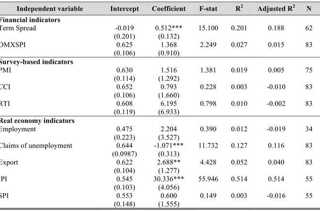
4.3 Regression models ... 34
5
Discussion ... 40
5.1 Financial indicators ... 40
5.2 Survey-based indicators ... 41
5.3 Real economy indicators ... 42
6
Conclusion ... 45
6.1 Limitations and Suggestions for Future Research ... 46
7
References ... 47
8
Appendix ... 53
8.1 Graphs before data transformations are conducted ... 53
Graphs
Graph 1 - Percentage Change in GDP - Term Spread ... 26
Graph 2 - Correct and Opposite Signals - GDP - Term Spread t-1 ... 26
Graph 3 - Percentage Change in GDP - OMXSPI ... 27
Graph 4 - Correct and Opposite Signals - GDP - OMXSPI t-1 ... 27
Graph 5 - Percentage change in GDP – PMI ... 28
Graph 6 - Correct and Opposite Signals - GDP - PMI ... 28
Graph 7 - Percentage Change in GDP – CCI ... 28
Graph 8 - Correct and Opposite Signals – GDP - CCI t-2 ... 29
Graph 9 - Percentage change in GDP - RTI ... 29
Graph 10 - Correct and Opposite Signals - GDP - RTI t-1 ... 29
Graph 11 - Percentage Change in GDP - Employment ... 30
Graph 12 - Correct and Opposite Signals - GDP - Employment t-2 ... 30
Graph 13 - Percentage Change in GDP - Claims of Unemployment ... 31
Graph 14 - Correct and Opposite signals GDP – Claims Of Unemployment ... 31
Graph 15 - Percentage Change in GDP - Export ... 31
Graph 16 - Correct and Opposite Signals - GDP - Export ... 32
Graph 18 - Percentage Change GDP - IPI ... 33
Graph 19 - Correct and Opposite Signals - GDP - IPI ... 33
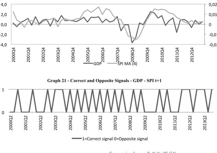
Graph 20 - Percentage Change in GDP - SPI ... 33
Graph 21 - Trend Adjusted – 4 Quarter Moving Average ... 34
Graph 22 - Correct and Opposite Signals - GDP - SPI t+1 ... 34
Tables Table 1 - Categories and Perspectives ... 5
Table 2 - Comprehensive Picture of Indicators ... 19
Table 3 - Data Transformation ... 21
Table 4 - Correlation ... 24
Table 5 - Cross-Correlation between GDP growth and Independent variables .... 25
Table 6 - Simple Linear Regression ... 35
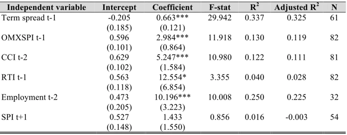
Table 7 - Simple Linear Regression Including Lag-Structure ... 36
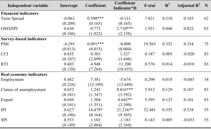
Table 8 - Simple Linear Regression Including Interaction Term ... 37
Table 9 - Explanatory Power Comparing Table 6 and Table 8 ... 37
Table 10 - Lag Structure with Interaction Term ... 38
Table 11 - Comparison Between Explanatory Power in Lag Structure from Table 7 and Table 10 ... 39
Table 12 – Summary - Empirical findings of indicators ... 44
Figures Figure 1 - Business Cycle ... 7
Appendix A. 1 - GDP and Term Spread ... 53
A. 2 - GDP and OMXSPI ... 53
A. 4 - GDP and CCI ... 54 A. 5 - GDP and RTI ... 54 A. 6 - GDP and Employment ... 54 A. 7 - GDP - Claims of Unemployment ... 55 A. 8- GDP and Export ... 55 A. 9 - GDP and IPI ... 55 A. 10 - GDP and SPI ... 55
A. 11 - Correct and Opposite Signals GDP - Term Spread ... 56
A. 12 - Correct and Opposite Signals GDP - OMXSPI ... 56
A. 13 - Correct and Opposite Signals GDP - CCI ... 56
A. 14 - Correct and Opposite Signals GDP - RTI ... 56
A. 15 - Correct and Opposite Signals GDP - Employment ... 57
1
Introduction
This chapter introduces the reader to the subject of this thesis. A background and problem discussion is provided, which lay ground for the purpose and research question of interest. In addition, delimitations and the outline for this thesis are presented.
After years of economic instability and financial crisis there is an increased attention towards the economic situation all over the world. In this context economic and business cycle indicators play an important role, since they provide information that state past, current and predict the future of a country’s economy. Indicators contain information that can help understand and forecast business cycles. Elliott, Granger and Timmermann (2006) argue that knowing the economy’s possible direction and events in advance will improve the process for decision makers. Government policy makers, economists, businessmen, investors, employees and consumers all rely on forecasts for future judgment and base their strategic decisions on this information (Zarnowitz, 1992). Therefore, it is important that economic indicators are reliable and provide accurate information in order for different players to interpret them correctly. In this thesis both economic and business cycle indicators is grouped under the name indicators.
Lately, the stability of Swedish indicators has been questioned. Research made by Boström (2013) at Danske Bank1, discuss the trustworthiness and stability of two economic indicators in Sweden; Purchasing Managers Index (PMI) and National Institute of Economic Research (NIER) business confidence. The cause of concern is their deterioration during the last few years. After the financial crisis in 2008 there has been an increase in inconsistent signals between survey and actual data of production. On the contrary, Bahlenberg (2013) reports that the divergences in data are not remarkable and these numbers have appeared before. The different views mentioned above raise the question of how economic indicators should be interpreted in the future. The authors of this thesis are interested to see if Boström’s argument is supported when observing a wider range of indicators.
Moore and Shiskin (1967) introduce a list of criteria that indicators should be evaluated on before they are selected for predicting the economy. Three of these will be observed in this study; “(1) economic significance in relation to business cycles, (2) statistical
1 Danske Bank is one of the players in the financial market that look at economic indicators
adequacy, (3) consistency of timing during business cycles” (p. 8). Based on the evaluation criteria, Hoagland and Taylor (cited in Kauffman, 1999), present stability as an important factor for indicators. Stability is the absence of randomness in indicators’ fluctuations compared to cyclical trends. When investigating consistent signals of indicators, they should follow the direction of the economy, GDP, in order to reflect the economic conditions.
In Sweden, GDP is published with a lag of 60 days after the end of each quarter. This data is also continuously revised and adjusted when new information is revealed (Statistics Sweden, 2014a). Therefore, there is an increased demand of forecasts, in order to explain the current situation and predict the direction of GDP. In this context, indicators are useful (Mitchell, 2009).
According to the authors of this thesis there is a lack of research about Swedish indicators. In order to analyse this further, the underlying hypothesis is to test whether Swedish indicators are stable over time. Furthermore, observe if stability changes before and after the financial crisis. For economist within the banking sector, among others, the generated findings could be important when making strategic decisions. In order to observe stability; Correct signal of up-and downturns in indicators compared to GDP is first graphed. Secondly, correlation and cross-correlation is implemented to observe where the direction and strength is strongest and get an understanding of indicators’ lag structure. Thirdly, regression analysis of GDP against each indicator is performed to understand their explanatory power.
1.1 Background
As previously stated, indicators play an important role for different decision makers. According to Riksbank (2011) the Swedish Central Bank use macroeconomic forecasts based on economic indicators when regulating the benchmark rate. Their mission is to keep inflation at a low and stable level for maintaining financial stability. All major banks in Sweden have research departments that analyze macroeconomic trends, regionally, nationally and internationally. The information is combined to give a broader view of where the economy is heading. For instance, Danske Bank Research (2014a) publishes analysis in order to give their institutional and corporate clients a deeper insight into the economic situation. The aim of the research is to help companies in their decision making process and to achieve higher performance (Danske Bank Research, 2014b). Another example is Insurance Sweden, an organization that develops a competitive market for insurance companies within Sweden. They analyse macroeconomic changes and focus on long-term investments for the ability to dampen cyclical fluctuations. Insurance companies’ role is to take over risks of individuals
and businesses and therefore need to know the economy in advance (Erlandsson, Friman & Ström, 2013). In addition, businesses look at predictions of the future economy to make decisions of employment and inventory needs (Zarnowitz, 1992).
Originally, Mitchell and Burns (1946; 1961) present a study of indicators. They introduce that indicators discover patterns of economic fluctuations which is defined as business cycles. In their first work they also list indicators according to their trustworthiness in relation to business fluctuations2. Furthermore, Mitchell and Burns (1946) identify movements in indicators with respect to their timing of business cycles, considered as leads and lags. This information is later used by Moore (1961) who divides indicators into groups of leading, coincident and lagging indicators.3 The author argues that there are two perspectives and the user needs to decide which one to obtain; less in depth information about the business cycles or irregular in depth information at an early stage. Indicators are also categorized according to their attributes and performance. Drechsel and Scheufele (2010) define some categories of indicators; financial, survey-based, prices and wages, real economy and composite indicators. The strength of financial and survey-based indicators is their availability to give early signals of the real economic situation. Clemen (1989) observes combined indicators and states that when combining indicators into an index, this provide more accurate forecasts compared to using single indicators. Composite indicators are for many researchers synonyms with combined indicators.
Moore (1961) renews Mitchell and Burns’ (1961) list of indicators, which is based on a study made from pre and post-war information. Indicators’ ability to describe and predict movements in business cycles change, where some leading indicators show coincident characteristics after the war. A major finding is that indicators after the war often exclude business cycles turns, which generate errors. Other indicators included more business cycle turns compared to the real economy. When it comes to indicators’ ability to signal an expansion or recession, Stock and Watson (2003a) conclude that every recession decline in a different way. Hence, indicators perform differently in each recession. Mitchell and Burns (1961) argue that this occur since indicators reflect different characteristics of economic activity. Therefore, different results of the same indicator can be obtained for different recessions in time.
2 This study later receives critique from Koopman (1947), who argue that the absence of a theoretical model in
their findings is a disadvantage for the analysis of economic fluctuations.
3 Moore (1961, p. 45) defines the classifications according to “their tendency to reach cyclical turns ahead of,
1.2 Problem Discussion
What can be seen during recent time is that PMI’s and NIER business confidence’s stability has deteriorated, which has caused concern among economists. Boström (2013) and Bahlenberg (2013) have different perspectives of the seriousness of the problem. However, despite the disagreement, economists and analysts use the information on a daily basis when making strategic decisions.
A problem seen in previous research is ambiguous findings regarding indicators’ stability. Most research has been conducted in the U.S. or with perspective of the U.S. economy. Scarce research has been made regarding Swedish indicators. However, the conducted research focuses mostly on the survey-based category and excludes other categories. Österholm (2014) publishes a research where the author observes the predictive ability of survey-based data in relation to Swedish GDP growth.
In Germany on the other hand, Drechsel and Scheufele (2010) observe a broader picture when predicting the economy. The authors focus on indicators within the categories; financial, survey, price and wages, real economy and composite indicators. With respect to this, it can be interesting to contribute in a similar manner, obtaining a Swedish perspective, by analysing a wide range of indicators.
An additional problem according to previous literature is that indicators’ consistencies over time have been questioned. Boström (2013) see changes in PMI and NIER business confidence since the financial crisis in 2007-2008. Moore (1961) suggests that major events like wars change the economy and the stability of some economic indicators. Both war and financial crisis are sources of economic disruption. When considering financial crisis, a similar effect on indicator as seen in pre-and post-war information can be possible. When observing a number of indicators with the same time period, this makes it possible to compare results across indicators and categories.
1.3 Purpose
The purpose of this research is to empirically study selected Swedish economic and business cycle indicators’ stability over time with respect to GDP growth. Stability is in this thesis defined as indicators ability to provide reliable, accurate and consistent signals of the economy’s direction, GDP. The aim is to get a better understanding of indicators’ ability to predict future movements in the economy. The effect of the financial crisis in 2008 will be used as a benchmark to see if there has been a change in indicators’ ability to predict GDP growth.
1.4 Delimitations
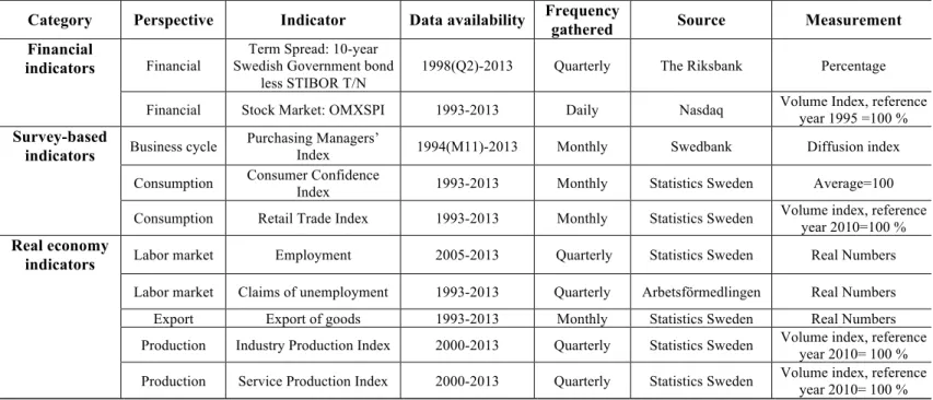
The focus is on Swedish indicators’, both economic and business cycle indicators, predictive ability against GDP. Ten indicators are selected with respect to the following criteria; the widespread use of economic indicators by different players in the market, important indicators according to previous studies and publicly available data. The authors have selected indicators that fulfil these criteria to get a broad perspective of the economy. The selected indicators are grouped into three categories; financial, survey-based and real economy indicators. The following indicators will be studied:
Table 1 - Categories and Perspectives
Category Perspective Indicator Data availability
Financial
indicators Financial Term Spread: 10-year Swedish Government bond less STIBOR T/N 1998(Q2)-2013
Financial Stock Market: OMXSPI 1993-2013
Survey-based
indicators Business cycle Purchasing Managers Index 1994(M11)-2013 Consumption Consumer Confidence Index 1993-2013
Consumption Retail Trade Index 1993-2013
Real economy
indicators Labor market Employment 2005-2013
Labor market Claims of unemployment 1993-2013
Export Export of goods 1993-2013
Production Industry Production Index 2000-2013
Production Service Production Index 2000-2013
Previous research of indicators in Sweden is limited; the literature focuses mostly on the U.S. and the overall European economy. Each country’s economy behaves differently and the indicators can therefore behave in different ways depending on the chosen country. However, these differences will not be considered in this thesis. The empirical findings will be connected to the Swedish market and conclusions will be drawn with respect previous research conducted in other countries than Sweden. Furthermore, some areas within the literature have recently been updated while this is not the case for all previous literature. Therefore, some previous literature included does not study the modern economy today. However, this thesis tries to capture the most prominent work of previous publications. During the last few decades, statistical models have also been developed with attempts to improve the composition of indicators that indicate movements in business cycles. Examples of such models are the dynamic factor model and pooled indicator. However, these will not be included in this study. The financial crisis in 2008 will be used as a benchmark for stability. The sample period includes additional financial crisis, these will not be considered. Further consideration in relation to stationary and nonstationary time series are not made. A visual examination of the graphs shows no sign of stationary. This thesis will study stability in
indicators, however it will not examine if the cause of potential deterioration in stability is due to the economy or the underlying mechanism in the indicator.
1.5 Outline
This thesis is divided into sections as follow: in section 2, previous research within business cycles and stability of economic indicators are presented. In section 3, the underlying methodologies and methods for the conducted research are explained. In section 4, empirical findings and basic analysis are presented, and in section 5 the empirical findings and previous literature more in depth are discussed. Finally, in section 6 the authors make concluding remarks, present limitations of the study and give suggestions for future research.
2
Theory and Previous Literature
In this section we present to the reader theories behind business cycles and its link to GDP. Furthermore, important milestones in the history and developments of economic and business indicators are presented. The aim of this section is to help the reader understand the context and use of indicators and their ability to signal economic changes and conditions. Different authors have tried to evaluate indicators, however scarce research has been conducted for some of the indicators.
2.1 Descriptive Information of Business Cycles
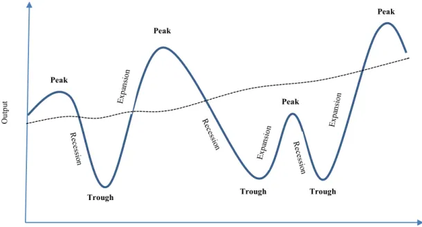
Business cycles are explained as the difference between actual GDP and the underlying trend. The underlying trend can be seen as potential GDP, which is obtained when the economy experiences full employment. The economy is in an expansion when actual GDP is above the underlying trend, and in a recession when actual GDP is below the trend. Turning points in the economy are named peaks and troughs, indicating the highest and lowest point that the economy can reach in the current economic condition (Fregert & Jonung, 2010). A whole business cycle is the period it takes for the economy to undergo both an expansion and recession, seen in figure 1. Furthermore, it can be seen as the economy’s way to react to different disturbances, derived from both supply- and demand side. One example could be changes in production or changes in demand for investment goods (Dornbusch, Fischer, & Startz, 2011)
Figure 1 - Business Cycle
Source: Authors’ own graph
Peak Peak Peak Peak Expa nsio n Re ce ssio n Re ce ssion Re ce ssio n Expa nsio n
Trough Trough Trough
Time Ou tp ut Expa nsio n
One of the oldest and most basic uses of national accounts is to measure the growth of an economy. Gross Domestic Product, GDP summarises a country’s economic position (Eurostat, 2012). GDP is the total value of all products and services that are produced within the borders of a country and are used in consumption, export and investment during a set period, normally one year. Foreign owned companies that produce goods within Sweden are included and domestic companies that produce goods abroad are excluded (Statistics Sweden, 2013a). A commonly used model in macroeconomics to describe GDP is defined as follow:
𝑌 = 𝐶 + 𝐼 + 𝐺 + 𝑁 (2.1)
Y is the demand for output in a country; C stands for consumption spending by households; I reflect businesses and households investment spending; G is purchases of goods and services by the government; N stands for foreign demand of a country’s net export. Indicators measure different economic factors and have therefore connection to the above formula (Dornbusch, Fischer, & Startz, 2011)
2.2 Business Cycle Theory
The most prominent work on business cycles is developed by Samuelson (1939) who combines different hypotheses into a coherent framework to describe market fluctuations. The theory is based on rigorous and mathematical approaches; the model is called multiplier-accelerator. This model shows that changes in purchasing power give rise to cyclical fluctuations. A basic description is that when purchase power rises, it leads to an increase in the multiplier-accelerator effect which initiates investment and generate further economic growth. When the economy experience maximum capacity, eventually production will slow down and investments fall. After a period of decline in production, various investments are made, which give rise to an upswing in the economy.
Keynes (2007) discusses ideas of how to dampen cyclical changes and points out the importance of striving to reach full employment. The author argues that there are no guarantee that produced goods will be required by consumers. Therefore unemployment can be a natural cause if there is lack in demand, especially during a downturn economic phase. Government spending should put underused savings into work in order to increase aggregated demand and hence economic activity. According to Keynes this would increase employment and decrease deflation.
Modern business cycle theory is based on two fundamental approaches; (1) there are predetermined elements in the economic cycle. The predetermined element makes GDP and economic indicators change in a low pace and the business cycles duration can last several
years. Therefore, no radical changes between subsequent quarters can be seen. (2) There are also random elements that can cause sudden events, which make the business cycle abruptly change direction (Fregert & Jonung, 2010).
To explain the two fundamental approaches, Frisch (1933) develops an impulse-propagation model. The economy is constantly exposed to external random disturbances, known as impulses. Different reasons why the disturbances appear can be increases in oil prices or changes in the worldwide economy. The economy’s process of adapting to these disturbances is slow and takes time. The impulse describes the random events in the business cycle and the slow adapting process describes the predetermined elements. The impulse-propagation model is used to distribute the impulse signals over longer time cycles through slow dispersal mechanisms. The business cycles lengths increase when the dispersal mechanisms are slower.
Cyclical movements in business cycles are normally between three and eight years (Fregert & Jonung, 2010). However, Kondratieff and Stolper (1935), Kuznet (1961) and Juglar (1862) provide research and argue for cycles that stretch over longer time periods. Kondratieff and Stolper (1935) discover cyclical waves ranging from forty to sixty years. The authors study developments in wholesale prices, wages and interest rates by using a smoothing average technique when eliminating trends in the economic times series. Kuznet (1961) observes cycles ranging from fifteen until twenty-five years. The author implements a more qualitative approach when including both physical production and price variation of commodities. Juglar (1862) studies changes in industrial economies by observing changes in fixed capital investments and find cycles ranging between seven and eleven years. Most economists today refer to these Juglar cycles when talking about business cycles.
2.3 Economic Indicators
2.3.1 Financial indicators
The interest of using financial indicators when forecasting economic activity has been present ever since Mitchell and Burns (1961) introduced Dow Jones composite index of stock price as a leading indicator. Extensive research include and discuss financial variables’ predictive ability and stability with respect to GDP growth, in different forms; term spread, stock price, dividends yield, interest and exchange rates (Stock & Watson, 2003b).
Stock and Watson (2003b) provide a literature review and empirical analysis of financial indicators. The authors find that instability is a common feature among financial indicators. Empirically, Stock and Watson (2003b) find that different financial indicators are
significant when marginally predicting GDP growth over different time periods. However, no financial indicator shows predictive ability over several sectors within different countries4. Financial indicators have good predictive power in one period while this is not always the case in the following periods. Term spread was the financial indicator that provided most stability over different time periods. The authors claim that financial indicators’ instability generally come from economic shocks, part of random fluctuations and development in financial systems.
Term spread
Bernanke and Blinder (1992) as well as Estrella and Mishkin (1997) claim that term spread is closely connected to a country's pursued monetary policies. When tightening monetary policies, higher short-term rates can be seen which generates a lower term spread and economic slowdown, and vice versa. When term spread increases, a positive change in GDP is predicted for the future (Ang, Piazzesi & Wei, 2006; Wheelock & Wohar, 2009).
Extensive researches have been conducted with respect to the US economy. Among those Estrella and Hardouvelis (1991), Wheelock and Wohar (2009), and Bernanke and Blinder (1992) argue that term spread forecast GDP growth. Estrella and Mishkin (1997) confirm that this also is true for the Euro area. Wheelock and Wohar (2009) conclude that researchers most common view are that term spread provide forecasting abilities, six to twelve months ahead of GDP growth. Estrella and Mishkin (1997) on the other hand observe different countries and claim that term spread, on average, has a predictive ability between one and two years. Wheelock and Wohar (2009) argue that term spread generally provides more reliable predictions in terms of recessions compared to growth in business cycles. It has the ability to predict a possible slowdown one year in advance. Estrella and Hardouvelis (1991) found that term spread performs better forecasts compared to survey-based indicators.
Stock price - Stock market
According to Stock and Watson (2003b), stock prices have been considered a forecaster of GDP growth during a long time. The use of stock price as an indicator is considered valid in macroeconomics since future earnings on stocks are argued to reflect the current stock prices. Hence, it indicates investors’ future expectations. Fisher and Merton (1984) argue that changes in stock prices both positive and negative, provide good forecasts. However, the
4 Stock and Watson (2003b) study seven countries; Germany, Italy, France, the UK, the US, Canada and Japan for a
majority of researchers claim the opposite. Both Drechsel and Scheufele (2010) and Stock and Watson, (2003b) argue that stock prices have shown empirically unstable results when predicting GDP. Estrella and Mishkin (1998) observe stock prices in relation to recessions. The authors’ results show that it accurately predicts a recession, one to three quarters ahead its occurrence.
2.3.2 Survey-Based Indicators
Österholm (2014) claims that survey data in the NIER Business Tendency Survey has “informational value” (p.135) and can improve short-term forecasts of Swedish GDP growth. Hansson, Jansson and Löf (2005) highlight important factors for survey-based indicators’ reliability in relation to GDP performance. Survey data is immediately available, have very few or no measurement errors and disregard the process of being revised.
Purchasing Managers’ Index - PMI
An increased value in PMI shows that manager reports successful business surroundings and have positive predictions of the future. However, the index does not capture the difference in sizes between companies and its related circumstances, which can explain why economic shifts sometimes are overlooked by PMI. The index is publicly available the first day during the next month and its timeliness is valuable as a first indication of economic change. Furthermore, it is considered to be a leading indicator (Koenig, 2002).
Kauffman (1999) finds that PMI has high correlation to GDP and lags the overall business cycle. Harris (1991) indicates that GDP does not follow a smooth development pattern, therefore PMI often shows peaks when the economy is recovering, and it also shows many smaller peaks during an upward phase of the economy. Correct signals in relation to recessions occur between zero and twenty month ahead an upturn, however irregularity in this aspect is also seen. Many economists use PMI as a signal of change and put less weight on its leading ability. Harris (1991) makes a summary of previous research, the findings supports that PMI indicates up- and downturns in the economy. However, there is little evidence that PMI actually provide new information, which is not provided by other indicators.
Consumer Confidence Index – CCI
CCI’s measure is based on economic optimism, expressed through consumers’ attitudes in relation to savings and consumption. These attitudes affect the economic aggregated demand. When CCI increases, consumption grows and higher demand for goods and services is seen,
which affect GDP (Dornbusch et.al, 2011). According to Ludvigson (2004) survey questions in CCI relate to consumers’ present situation and contain meaningful information. Hence, it is used as a benchmark for the current economic level. Taylor and McNabb (2007) show that CCI are procyclical and have a significant impact when predicting downturns in the economy. Authors such as Carroll, Fuhrer and Wilcox (1994) and Matsusaka and Sbordone (1995) analyze CCI to see if it provides additional information in relation to other economic indicators. The authors find that CCI has important explanatory power for fluctuations in GDP, even when other macroeconomic variables are considered. On the contrary, Al-Eyd, Barrell and Davis (2009) see decreasing predictability in CCI and question its reliability. Batchelor and Dua (1998) findings show that including CCI can increase the chance of discovering a recession and highlight its ability to see economic fluctuations.
Retail Trade Index - RTI
In the American market, Retail Trade Index investigates the dollar value of goods sold in the retail trade industry. Retail Sales Index is closely linked to Retail Trade Index and is observed by many economists. Its aggregated value makes up for two-thirds of the overall GDP. It reflects the current economic state, and therefore is included as a coincident indicator. Furthermore, it is also valuable when measuring the inflation rate (Winton & Ralph, 2011).
2.3.3 Real Economy
Banbura and Rüstler (2011) observe the relation between hard and soft data when forecasting short-term GDP growth in the Euro area. Soft data reflect expectations while hard data state what actually happens in real numbers. Survey data are included in the higher frequency data section and are categorized as soft data, while hard data observe specific mechanisms in GDP. Differences in lag structure impact the number of correct signals in relation to GDP. When ignoring lags of publications, hard data provide more information with precise signals. When including differences in lags, hard data decrease its relevance and soft data have a higher impact on the forecast.
Employment / Claims of Unemployment
Drechsel and Scheufele (2010) argue that labor market indicators can be useful when studying GDP growth. The authors discuss unemployment rate, employment and vacancies in the labor market as leading indicators. Banerjee, Marcellino and Masten (2005) especially point out the following indicators; unemployment rate, employment, claims of unemployment and hours worked to best forecast GDP growth.
The relationship between GDP and labor market is widely recognized. As previously stated in section 2.1, the unemployment output “gap” represents differences between potential and actual economic output. Furthermore, Potential output exists when the economy experiences full employment. When the unemployment rate rises, GDP declines and vice versa (Friedman & Wachter, 1974). The reason for this relationship to exist is that higher cost of unemployment is considered as productivity loss for a country. If people do not work, the country decreases its production levels and less tax is generated for the government (Dornbusch et.al., 2011). However, Galvin and Kliesen (2002) argue that this relationship tends to hold in recessions but not over the whole business cycle and is therefore not a reliable predictor of GDP growth. The reason is due to changes among some microeconomic variables. The number of people being employed or unemployed is affected by demographics, unemployment benefits as well as cultural and social structures in the society. Dornbusch et.al (2011) add inflexibility in labor markets, especially in Europe, as an effect on unemployment and thereby its relationship to GDP. Real wage changes tend to move slowly, there are often high costs included when firing employees; this tends to keep unemployment at higher levels. The labor market can therefore have an extensive effect on the economy in recessions due to reluctance of hiring people.
Stock and Watson (1999) argue that employment is strongly procyclical. Additionally the authors state that employment has a lag of about one quarter with respect to the business cycle. However, Stock and Watson (2003a) argue that employment serve as a coincident indicator.
Stock and Watson (1999) argue that new unemployment claims lead the business cycle. Stock & Watson (2003a) argue that claims of unemployment is and have been an early indicator of when the business cycle is entering a downward phase. According to Montgomery, Zarnowitz, Tsay and Tiao (1998) this economic indicator include valuable information and leading abilities since it signal what direction unemployment will take in the following months.
Export of Goods
In equation (2.1) in previous section, N in relation to GDP represents net export and can either have a positive or negative impact on GDP, depending on the country’s export levels. Countries strive to increase the levels of production in order to generate a positive net export. The mechanism behind the ability to achieve a higher export is closely connected to a flexible exchange rate (Feenstra & Taylor, 2011).
Previous research among export and economic growth are divided into two sections. First, trade strategies and their effect on economic performance are examined, together with changed policies of export. Secondly, the relationship between increased levels of export and further economic growth are observed (Kavoussi, 1982). More emphasis in previous literature has been made with respect to the latter section. Tyler (1981) claims that understanding the importance of export can lead to increased investment levels in more effective sectors of the economy, thus generating improved productivity.
Karpaty and Kneller (2011) argue that Sweden’s economic growth is largely due to internationalization through foreign invested capital and increasing levels of export. Some evidence confirms that there is a positive relationship between increased amount of exports and productivity. Furthermore, this generates benefits from large scale of production.
Industry Production Index/ Service Production Index
Production has through out history been used in various forms as indicators to predict the economic direction and GDP growth. Moore (1961) introduces manufacturing, new orders and durable goods, which is part of production as leading indicators for business cycles in the U.S. Banbura and Rüstler (2011) argue that since production indices (both industrial and service production) are based on real activity with real numbers, the availability of data is delayed. This can delay information about GDP, however, they give accurate signals of GDP.
Production consists of a process where inputs, like material, is transformed into output and is generated to products. The relationship between input and output depends partly on production technology. This is something that is rapidly developing, and it constantly changing the means of production efficiency (Rasmussen, 2013).
According to Hosley and Kennedy (1985) the industrial sector together with construction represent the main variation in output. By analyzing the industrial production, structural changes in the economy can be measured and clarified. The Industry Production Index therefore reveals detailed information on different components in industry sectors. Furthermore, the authors highlight a close relationship between growth in industrial production and the exchange rate as well as a country’s trade deficit. A strong domestic currency and trade deficit commonly leads to growth in the industrial production sector.
Indices that measure service production have received increased attention during past decades. Moore (1991) discusses service industries and their increased economic importance. The reason for its increased importance is a rise in employment levels within the sector; hence it contributes more to GDP compared to previous decades. The author argues that growth
rates in indices based on service industries strongly move in the same direction as business cycles. Nowadays they have a complementary role in relation to industrial production when explaining countries’ fluctuations in the total economic output, which determine the direction of short-term movements (OECD, 2007). Layton and Moore (1989) argue that the service sector is more stable compared to industry production especially during recessions since there is no need for inventory. Additionally, the authors discuss services to be based mainly on demand, whereas both demand and supply play an important role in industry production.
3
Methodology, Data and Descriptive Statistics
In this section the philosophical basis of the chosen research method will be presented. The authors will illustrate how the empirical methods will be conducted, including data gathering, data arrangement and statistical methods that will be used. This chapter will also conclude a section where validity, reliability and generalizability of this thesis are discussed.
3.1 Research Philosophy, Approach and Design
The research philosophy is connected to the knowledge development of the research. It reflects the way a specific research view the world. There are three main philosophies; positivism, realism and interpretivism in the current literature (Saunder, Lewis & Thornhill, 2012). This thesis will obtain positivism as a philosophical standpoint. According to Saunders et al. (2012) data is collected from reality and is analysed in order to see relation and common features. This information is considered as generalized laws for researchers. Through this philosophy, we aim to establish if there is stability between economic indicators and GDP.
Research approaches reflects the way theory is used, there are three different approaches; deduction, induction and abduction (Saunders et al., 2012). This study will be based on a deductive research approach. The selected approach will include some of the main characteristics that Saunders et al. (2012) define when explaining the deductive research. The approach first involves developing a hypothesis based on previous research, which is later tested. It tries to explain the relationship between variables, additionally it is generalised through selecting a large data set. It is also possible to conduct an abductive approach, where new theories are developed by identifying patterns based on explaining facts. However, this is not illustrated in this thesis since it is not in line with the purpose.
Research design, sometimes referred to research strategy, involves the structure, outline and framework of the research being conducted. Often the research is exploratory, descriptive or casual design, also called explanatory design (Cooper & Schnidler, 2011). For this study, a descripto-exploratory research design is most suitable. Saunders et al. (2012) argues that the use of this design will link descriptive and explanatory views together. Firstly through calculations describing the data and then by providing interpretations of the relationships. A quantitative research method with secondary data will be conducted. This research method investigates the relationship between variables (Stock & Watson, 2012).
3.2 Method
3.2.1 Selection of Data and Test Period
Ever since Mitchell and Burns (1961) introduced the first list of useful economic indicators, the list has been revised over the years. The authors of this thesis will use previous research as a compliment when deciding which indicators to study. Further information with respect to Sweden will be gathered from Statistics Sweden, they publish and provide information of the most frequently used indicators. In relation to this, further research will be conducted to see which indicators that are used by the Central Bank in Sweden, other major banks, institutions, the insurance sector and companies. Indicators will be selected from the following three categories; Financial, Survey-based and Real economy. Stock and Watson (1999) analyze a wider range of indicators and classifie them into different perspectives based on the economic sector they belong to. From their way of classifying indicators, similar perspectives will be implemented.
The sample period will be based on publically available data. GDP will be used as dependent variable and indicators as independent variables. The test will include a maximum of 20 years since GDP is available from the first quarter of 1993 until the last quarter of 2013. However, indicators have different introduction dates and variety of length. Therefore some indicators have shorter time periods and the data will be included since they first were published. Exports, Claims of Unemployment, CCI and RTI are included from 1993 and cover the whole time frame of 20 years. IPI, SPI, Employment, OMXSPI, Term Spread and PMI cover different shorter time periods.
3.2.2 Data Gathering
The authors gathered information from the original sources. Seasonally adjusted GDP, IPI, SPI, Export, Employment, CCI and RTI are collected from Statistics Sweden. Claims of Unemployment from Arbetsförmedlingen, OMXSPI from NASDAQ, Term spread from the Riksbank (the Swedish central bank) and PMI from Swedbank.
3.2.3 Independent Variables –Indicators
Financial Indicators
Term Spread is the difference between long-term and short-term interest rate on maturity debt. There are different types of measures for term spread that can be used. The most common measures are long-term government bond rate less three-month government bond and long-term government bond rate less overnight rate (Stock & Watson, 2003b). This thesis uses the latter, where 10-year Swedish Government Bond rate is taken minus STIBOR N/A.
OMXSPI includes all companies’ shares in the stock market, listed on OMX Nordic Exchange Stockholm. It is an aggregated measure of the overall current value and changes of the stocks, combined into an index (The NASDAQ OMX Group Inc., 2014).
Survey-based Indicators
Purchasing Managers Index (PMI) is a qualitative survey where about 200 purchasing managers in the manufacturing industry in Sweden are interviewed. It reflects the companies’ current condition and the purchasing managers’ opinions of the near future, with respect to changes from the previous month. The aggregated information in relation to order intake (30 %), production (25 %), employment (20 %), supplier’s delivery time (15 %) and inventory (10 %) are combined into a diffusion index (Swedbank, 2014).
Consumer Confidence Index (CCI) is part of the Economic Tendency Survey, where 1500 Swedish households are asked questions about their economy (NIER, n.d.). Four questions on participants’ personal finances are averaged into representing CCI. Additionally, it includes participants’ view of the current and future Swedish economy for up to 12 months ahead. Lastly, a question is asked if they think it is a good time to buy consumer goods (Statistics Sweden, 2014b).
Retail Trade Index (RTI) is published every month and reports total retail sales development. It is based on the total revenue, including taxes and excluding exports. The survey is one of the primary sources when it comes to calculating private consumption in GDP (Statistics Sweden, 2013b)
Real economy Indicators
Employment is the number of people employed, both men and women in the age of 15-74 years old. Permanent and temporary employment as well as self-employment is included. Employment is part of the Labour Force Survey (Statistics Sweden, 2014c).
Claims of Unemployment is when employers give an early redundancy notice
employees within the companies. All claims of unemployment is collected and added for Sweden. However, companies only need to report reduction of employees when the number is at least five people. Therefore, the statistics do not include reductions less than five people (Arbetsförmedlingen, 2014).
Export includes the total value in Swedish Krona of all exported goods (Statistics Sweden, 2014c).
Industry Production Index (IPI) is a volume index designed to measure the industrial changes in the economy. It measures the industrial contribution to GDP between
two time periods. Data from mining, manufacturing, electricity, gas and heat are reported. IPI include three main data sources in the production sector; deliveries, hours worked and price changes (Statistics Sweden, 2013d).
Service Production Index (SPI) measures the growth of production within the service sector. SPI include data from trade, hotel and restaurants, transport, storage and communication, business services, education, health and care services and other services. The different components in SPI are selected based on consistency over time and cover a widespread of sectors (Statistics Sweden, 2008).
Table 2 - Comprehensive Picture of Indicators
Category Perspective Indicator Data availability Frequency gathered Source Measurement Financial
indicators Financial Swedish Government bond Term Spread: 10-year less STIBOR T/N
1998(Q2)-2013 Quarterly The Riksbank Percentage Financial Stock Market: OMXSPI 1993-2013 Daily Nasdaq Volume Index, reference year 1995 =100 % Survey-based
indicators Business cycle
Purchasing Managers’
Index 1994(M11)-2013 Monthly Swedbank Diffusion index Consumption Consumer Confidence Index 1993-2013 Monthly Statistics Sweden Average=100 Consumption Retail Trade Index 1993-2013 Monthly Statistics Sweden Volume index, reference year 2010=100 % Real economy
indicators Labor market Employment 2005-2013 Quarterly Statistics Sweden Real Numbers Labor market Claims of unemployment 1993-2013 Quarterly Arbetsförmedlingen Real Numbers Export Export of goods 1993-2013 Monthly Statistics Sweden Real Numbers Production Industry Production Index 2000-2013 Quarterly Statistics Sweden
Volume index, reference year 2010= 100 % Production Service Production Index 2000-2013 Quarterly Statistics Sweden
Volume index, reference year 2010= 100 %
3.2.4 Data Arrangement and Quality
The data chosen for this study have different underlying measures5. Indicators that are presented in volume indices are constructed in the same way but have different base periods. In order to make correct comparisons between GDP and index numbers6, the base period will be changed (Aczel & Sounderpandian, 2009). GDP use the fourth quarter of 2012 as a base period, the indicators will therefore be transformed into the same period. The following formula will be used to change the base period for the indices:
𝑁𝑒𝑤 𝑖𝑛𝑑𝑒𝑥 𝑣𝑎𝑙𝑢𝑒 = !"# !"#$% !"#$%
!"#$% !"#$% !" !"# !"#$ × 100 (3.1)
5 Index, Diffusion index, Real number and Percent.
6“Index number is a number that measures the relative change in a set of measurements over time”, to construct
a simple index, a base year is chosen and the index number is the percentage of the ratio between two values, the current value divided by the value of the base year, times 100 (Aczel & Sounderpandian, 2009, p 583)
The indicators that will be used are either released daily, monthly or quarterly. OMXSPI is released on a daily basis while Export, CCI, RTI and PMI are released monthly. IPI, SPI, Claims of Unemployment, Employment and Term Spread are released quarterly together with GDP. In order to compare economic indicators with GDP, the indicators released on a daily or monthly basis will be transformed into representing quarterly data. This procedure differs depending on the underlying measure. Export is release in real numbers on a monthly basis and will therefore be aggregated by adding together three months’ data for each quarter. When consider indices, diffusion indices or survey-based measures, the last date or month in each quarter will be included. This facilitates the procedure of making direct comparisons. An alternative approach is to use three months average value in each quarter. However by doing so, important information about fluctuations in the indicators can be overlooked.
GDP growth measures the percentage change in GDP from one period to the next. Logarithmic Transformation, with natural logarithm, will be conducted on the data of indicators, while the percentage change for GDP will not include a logarithmic transformation. In developing economics it is common to use logarithmic transformation to get GDP growth (Stock & Watson, 2012). However, since Sweden is considered a developed country, it is said not to experience exponential growth. Therefore the growth will not include a logarithmic transformation.
∆𝑦! = 𝐿𝑁 !!
!!!! (3.2)
7
When observing a diffusion index8, the absolute change in relation to the previous period is already measured. Hence, errors will appear if this data is transformed into representing percentage change. Therefore, the absolute number of diffusion index will be used, without any changes. Previous literature considers the absolute level of the spread, the same will be considered here.
7 ∆𝑦!= 𝐿𝑁 !!
!!!! = 𝐿𝑁 𝑦!− 𝐿𝑁 𝑦!!!
8 A diffusion index ranges between 0-100. 50 defines no change (50 percent of the firms/industries experience
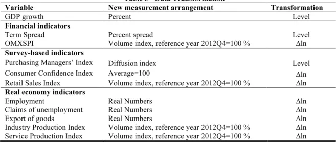
Table 3 - Data Transformation
Variable New measurement arrangement Transformation
GDP growth Percent Level
Financial indicators
Term Spread Percent spread Level
OMXSPI Volume index, reference year 2012Q4=100 % ∆ln
Survey-based indicators
Purchasing Managers’ Index Diffusion index Level
Consumer Confidence Index Average=100 ∆ln
Retail Sales Index Volume index, reference year 2012Q4=100 % ∆ln
Real economy indicators
Employment Real Numbers ∆ln
Claims of unemployment Real Numbers ∆ln
Export of goods Real Numbers ∆ln
Industry Production Index Volume index, reference year 2012Q4=100 % ∆ln Service Production Index Volume index, reference year 2012Q4=100 % ∆ln
3.3 Statistical methods
3.3.1 Correlation and Cross-Correlation
To examine the chosen economic indicators’ change associated to GDP growth, correlation between these will be tested. Correlation is a non-unit measurement that indicates the strength and direction of an association between two variables. The measure of correlation is expressed as values between -1 and 1. The value of 0 indicates no association between variables, -1 indicates a maximum negative relationship and 1 show a maximum positive relationship (Stock & Watson, 2012). This test will provide information of the linear relationship between indicators and GDP growth. A high positive correlation will indicate that two variables move in the same direction, whereas the opposite is true for a negative correlation.
Cross-correlation is an extension of correlation that is used to study similarities in waves for time series that have cyclical movements. Cross-correlation measure the correlation between two time series when one of them either lead or lag, Xt-1 or Xt+1. It is useful to
determine how indicators signals are correlated with respect to lag structure for an up- or downturn movement in GDP growth (Chatfiels, 2004). This test will also give information of specific indicators and their ability to serve as leading, coincident or lagging indicator. Cross-correlation is beneficial as a measurement since its relation to trends does not need to be considered. The test can be implemented regardless of stationary or non-stationary in time series (Taylor & McNabb, 2007).
3.3.2 4 quarters moving average - MA (4)
There can be irregular patterns in time series, which decrease consistency and show irregular movements. Sometimes a visual understanding of a plotted time series can be difficult to
interpret. When smoothing the time series using a moving average, the picture gets clearer. The idea behind the concept is that large irregular movements at any point in time will generate less effect if they are averaged together with four quarters, totally representing a year. The seasonal effects are combined and shown through one seasonal moving average. (Newbold, Carlson, & Thorne, 2013).
A visual interpretation of the plotted graphs will be made under the section empirical findings. After this, a decision will be made if some of the indicators need to be adjusted with moving average. For these indicators, these values will be used in addition to the original data in the Correlation and Cross-Correlation tables.
3.3.3 Regression Models
The purpose of this thesis includes testing if economic indicators’ predictive ability has changed, after the financial crisis, in relation to GDP growth. First a simple linear regression model (3.3) will be conducted. It shows the relationship between the dependent and independent variable with respect to the whole time period. 𝛽! is where it intercept Yt and 𝛽! indicate the slope of the line. Later, an additional regression model will be included with an interaction term of a continuous variable multiplied with a binary variable, representing the time period after the start of the financial crisis (Aczel & Sounderpandian, 2009).
𝑌! = 𝛽!+ 𝛽!𝑋! + 𝑢! (3.3)
𝑌! = 𝛽!+ 𝛽!𝑋!+ 𝛽!(𝑋!×𝐷) + 𝑢! (3.4)
The above-mentioned tests will be conducted for each economic indicator. The binary variable D, also named dummy variable, is denoted 0 for the time period before the financial crisis and 1 from the second quarter of 2008 until the end of the test period. Focus is to examine the indicators’ explanatory power in relation to GDP.
The level of significance in the tested variables measures the probability that the true beta value lies within a specific confidence interval. The standard significant values are 1%, 5% and 10%. If the p-value falls below the chosen significance level, H0 will be rejected. A
significant level of 10 % equals the probability that the true coefficient value lies within a 90 % confidence interval; a similar interpretation can be made for other levels of significance (Aczel & Sounderpandian, 2009).
R2 shows how much of the dependent variable that is explained by the independent
variable. It could also be used to describe how well the regression line and data coincide. R2 is
always between 0 and 1 and its interpretation is made in percentage. When more independent variables are added to the equation, R2 increases. To adjust for this increase, adjusted R2 can
be observed when different numbers of independent variables are included (Aczel & Sounderpandian, 2009).
3.3.4 Consistent and Opposite Signals
To observe if the indicator give correct or opposite signals in relation to GDP. A function is used that show signal 1 if the indicator move in the same direction as GDP does. It signals 0 when the indicator moves in the opposite direction. However, when it comes to PMI and Term Spread, a positive change in PMI is above 50 while a negative change is below 50. Term Spread indicates a positive change when the absolute level has increased from the previous quarter. A negative change can be seen when it decreased from the previous quarter.
3.3.5 Validity, reliability and generalizability
To ensure that correct data have been used, the secondary data is collected from original sources. Furthermore, all data are checked twice to ensure accuracy. Cooper and Schnidler (2011, p.280) define reliability as “accuracy and precision of a measurement procedure”. With respect to this, reliability empirical findings are conducted. The study intends to measure stability and the conducted tests capture the changes in indicators. The statistical tests are performed to observe stability and the underlying hypothesis can therefore be answered. This ensures validity by measuring what is intended to measure (Cooper & Schnidler, 2011). The authors want to highlight the possibility that the empirical findings in this thesis may not be subject to generalizability if similar tests will be conducted with different samples. The reason for this is findings in previous literature, where no consensus has been made with respect to indicators’ stability. When it comes to practicality and usefulness, the concluded result provided a first overview of indicators’ stability. However, it can be considered that users of the empirical findings in this thesis conduct a deeper research on the specific indicator of interest before it is implemented in the decision-making processes.
4
Empirical Findings
In this section empirical findings in form of tables and graphs will be presented based on the selected methods in previous section. Descriptive text to illustrate the tables and graphs is included, in addition to some basic analysis of what can be seen. This section is divided into sub-sections based on the different statistical methods used; Correlation and Cross-Correlation, Visual interpretation with Graphs and Correct/Opposite Signals, and finally Regressions. Tables and graphs are the authors own construction based on the collected data.
When interpreting the empirical findings, the authors use the terms reliable, accurate and consistent, in order to analyse stability. Accuracy is used to describe indicators’ explanatory power, R2. To check for reliability, the correct and opposite graphs are observed to see if the indicator moves in the same direction as GDP. Lastly, consistency is used to observe if indicators follow GDP’s direction over time. Here indicators’ significance in the regression models is analysed.
4.1
Correlation and Cross-correlationTable 4 illustrates correlation between GDP growth and each indicator. Exports of goods and SPI, show seasonal fluctuations (see graphs 15 and 20 respectively, in section 4.2). Therefore, these time series are adjusted with four quarter moving average. The table below includes the moving average correlation to show its enhanced correlation when adjusted for seasonal movements.
Table 4 - Correlation
Independent variable Correlation Correlation MA* Financial indicators Term Spread 0.448 OMXSPI 0.164 Survey-based indicators PMI 0.593 CCI 0.053 RTI 0.099
Real economy indicators
Employment 0.110
Claims of unemployment -0.356
Export of goods 0.228 0.562
IPI 0.717
SPI 0.053 0.571
GDP growth as dependent variable *Moving Average (4)
Term Spread, PMI, and IPI show relatively high positive correlation with GDP growth. This means that changes in indicators follow changes in GDP. IPI is the economic indicators that best follow GDP growth by 71,7 %. Claims of unemployment indicate a negative correlation,