Working Paper 2009:18
Department of Economics
Lending Relationships and
Monetary Policy
Yunus Aksoy, Henrique S. Basso and Javier
Coto-Martinez
Department
of
Economics
Working
paper
2009:18
Uppsala
University
December
2009
P.O.
Box
513
ISSN
1653-6975
SE-751 20 Uppsala
Sweden
Fax: +46 18 471 14 78
L
ENDINGR
ELATIONSHIPS ANDM
ONETARYP
OLICYLending Relationships and Monetary Policy
∗Yunus Aksoy†, Henrique S. Basso‡ and Javier Coto-Martinez§
October 2009
First version April 2009
Abstract
Financial intermediation and bank spreads are important elements in the analysis of business cycle transmission and monetary policy. We present a simple framework that introduces lending relationships, a relevant feature of financial intermediation that has been so far neglected in the monetary economics literature, into a dynamic stochastic general equilibrium model with staggered prices and cost channels. Our main findings are: (i) banking spreads move countercyclically generating amplified output responses, (ii) spread movements are important for monetary policy making even when a standard Taylor rule is employed (iii) modifying the policy rule to include a banking spread adjustment improves stabilization of shocks and increases welfare when compared to rules that only respond to output gap and in-flation, and finally (iv) the presence of strong lending relationships in the banking sector can lead to indeterminacy of equilibrium forcing the central bank to react to spread movements.
JEL Codes: E44, E52, G21
Keyword: Endogenous Banking Spread, Credit Markets, Cost Channel of Monetary Transmission, Firm-bank Relationships
∗We would like to thank Paul de Grauwe, Nils Gottfries and seminar participants at the
Bank of England, Bank of Finland/CEPR Conference in Helsinki, Riksbank, Cagliari University, Catholic University of Leuven and Uppsala University for comments. The usual disclaimer applies.
†School of Economics, Mathematics and Statistics, Birkbeck, University of London, Malet
Street, WC1E 7HX, London, United Kingdom, Tel: +44 20 7631 6407, Fax: +44 20 7631 6416, e-mail: yaksoy@ems.bbk.ac.uk
‡Corresponding Author. Department of Economics, Uppsala University, P.O. Box 513,
SE-751 20, Uppsala, Sweden, e-mail: henrique.basso@nek.uu.se
§Department of Economics and Finance, Brunel University, Uxbridge, Middlesex, UB8 3PH,
1.
Introduction
There has been a recent focus on the effects of financial intermediation, and more particularly on the impact of different short term interest rates on economic and monetary policy analysis. The main contributions to the literature can be divided into two clusters: one that focus on including a banking sector that produces loans and deposits following Goodfriend and McCallum (2007) and one that focus on the costly state verification approach of Bernanke, Gertler, and Gilchrist (1999) and Carlstrom and Fuerst (1997). Lending or firm-bank relationships, however, have been so far neglected.
Lending relationships are directly aimed at resolving problems of asymmetric information as identified by Diamond (1984). In order to obtain better borrowing terms a firm might find optimal to reveal to its bank proprietary information that is not available to the financial market at large. Banks will have the incentive to invest in acquiring information about a borrower in order to build a lasting and profitable association. That way, the information flow between banks and firms improve, increasing the added value of a firm-bank relationship (see amongst oth-ers, Boot (2000) and Petersen and Rajan (1994)). On the other hand, as pointed by Rajan (1992), such relationships also have a (hold-up) cost. After a relation-ship is formed banks gain an information monopoly that increase their bargaining power over firms. Santos and Winton (2008), using data from the US credit mar-ket, show that banking spreads can increase up to 95 basis points in a recession due to the fact that banks exploit this informational advantage after relationships are formed. Hence, banking spread movements driven by the existence of these relationship are significant and add to the “bank channel” effect of business cy-cle transmission and monetary policy. The hold-up or locked-in problem is also emphasized by the European Commission report on the banking sector (Euro-pean Commission (2007)). They conclude that competition problems within the industry are exacerbated as a result of information asymmetries between banks and their customers, which contribute to increasing switching costs. Finally, De-gryse and Ongena (2008) and references therein present empirical evidence of the positive link between lending relationships and bank rents.
The primary objectives of the present paper are to provide a simple theo-retical framework that augments the standard New Keynesian model to include lending relationships and to analyze its effect on credit market outcomes and eco-nomic activity. In our model, demand for credit is determined by working capital
assumptions. Firms must borrow to pay for the capital input and salaries, thus they are subject to cost channels of monetary transmission. In order to intro-duce lending relationships we assume that each firm selects a set of banks to acquire those funds from, but it has a preference to continue doing loans with the banks it traded with in the previous period. These preferences introduce an implicit switching cost that, although not modeled here, reflect greater infor-mational asymmetries with other borrowers. Hence, we do not explicitly model the hold-up problem but, similarly to Ravn, Schmitt-Grohe, and Uribe (2006), adopt a framework that reproduces a customer market effect in the baking sector. Given these intrinsic preferences banks gain market power, as a fraction of the current loan demand is not interest rate sensitive.
In line with the empirical evidence presented by Santos and Winton (2008) and Aliaga-Diaz and Olivero (2007), our model generates countercyclical banking spreads due to the existence of firm-bank relationships. When output and loan demand are high, banks are willing to decrease the banking spread to form as many relationships as possible. That reflects the fact that banks recognize that higher current demand leads to higher future loan demand. However, as out-put decreases, banks exploit the relationships already formed, increasing banking spreads and sustaining a higher profit margin during a downturn. The cyclical properties of banking spreads lead to two main corollaries. First, given an ini-tial shock that dampens output, banking spreads tend to increase. Loan interest rates, which are part of the firm’s current marginal and capital investment costs, also increase. As a result, investment and total production decrease further lead-ing to an amplification of output responses. This result is similar in nature to the financial accelerator proposed by Bernanke, Gertler, and Gilchrist (1999). In our model the amplification is a direct effect of the bank relationship and the cost channel, particularly on investment, while in Bernanke, Gertler, and Gilchrist (1999) it arises due to movements in firm’s net worth.
Second, the stronger the firm-bank relationships in the economy, the higher the banking spread response will be to an initial shock in output and loan de-mand. Higher banking spreads further dampens loan demand, leading to a new round of banking spread adjustments. If banking spreads are volatile enough, this process does not converge and the economy does not have a unique local rational expectations equilibrium. This feature is directly related to the fact that a significant portion of the loan demand is not interest rate sensitive. We show that there are, in principle, at least two ways to ensure determinacy. One is to
assume adjustment costs in the relationship banking, i.e. while firm-bank relation-ships are strong, banks also have a cost of maintaining relationrelation-ships. The basic motivation to include such costs would be that sharp spread movements might trigger firms to break the relationship and search for other banks. For instance, Ongena and Smith (2001) provide evidence that firms occasionally break lend-ing relationships. Alternatively and possibly more relevant for policymaklend-ing, we obtain determinacy if we allow the monetary policy to follow a spread-adjusted Taylor rule. If sharp banking spread changes are matched by base rate cuts, the final loan interest rate does not increase as much and the output-banking spread spiral that leads to indeterminacy does not occur. This result indicates that not only stabilization but also determinacy should be a concern for monetary policy in economies where competition in the banking sector is imperfect and lending relationships are present.
Finally, our analysis also sheds light on the effects of endogenous banking spreads on monetary policymaking. We initially assume that the central bank base rate only responds to inflation and output, employing a standard Taylor rule. Although not directly, the base rate responds to spread changes given its impact on output and inflation. We find that after a supply shock that leads to an increase in spread of around 110 basis points, the base rate response is 60 basis points lower compared to the constant spread case. Therefore, rein-forcing the results in Goodfriend and McCallum (2007), we conclude that ignor-ing the effects of bankignor-ing sector characteristics on monetary policy could lead to sub-optimal policy responses. Following Taylor (2008) we verify whether a spread-adjusted monetary policy improves stabilization. We find that respond-ing directly to spread movements may curb the output amplification observed in the presence of firm-bank relationships without increasing inflationary pres-sures. Furthermore, following Schmitt-Grohe and Uribe (2004a), we employ a second order approximation to welfare, and show that when banking spreads are endogenous, responding to spread movements leads to an improvement in welfare. As mentioned earlier a number of other studies have already proposed changes to a standard staggered pricing DSGE model to include different types of credit frictions and/or financial intermediation where a wedge between short term in-terest rates play an important role. Curdia and Woodford (2008), for instance, assume credit spreads between the loan and the central bank base rate that might change with credit aggregates loosely motivated by costly state verification. They find that movements to the spread are important for policymaking and that a
spread-adjusted Taylor rule, although not optimal, may improve stabilization. Assuming different effective discount factors they are able to ensure the same agent type lends and borrows, without the need of separating the agents that make deposits (households) and loans (firms) as most of the other contributions do. However, the endogeneity of spreads are ad-hoc and the monetary transmis-sion is via the consumption Euler equation without a consideration of investment and cost channels. De Fiore and Tristani (2008) also analyze optimal monetary policy in the presence of credit frictions derived from a costly state verification set-up. As Aliaga-Diaz and Olivero (2007) show banking spreads are countercycli-cal after controlling for credit spread changes indicating that the characteristics of the banking sector that we focus here are important determinants to the wedge between loan and base rates. Hulsewig, Mayer, and Wollmershuser (2006) and Teranishi (2008) also focus on the characteristics of banking sector on a model of cost channel similar to ours. However, their main assumption is that loan contracts are changed in a staggered fashion, while we focus on the endogeneity of banking spreads due to lending relationships.
The paper’s outline is as follows. Section 2 presents the model. In section 3 we begin by presenting the equilibrium conditions and then focus on the lin-earized system of equations and the parameters used in the numerical analysis. Section 4 presents the model’s main dynamic properties and the results of our policy experiments. Section 5 considers the determinacy properties of our model economy. Finally, Section 6 concludes.
2.
Model
The economy consists of a representative household, a representative final good firm, a continuum of intermediate good firms i ∈ [0, 1], a continuum of banks j ∈ [0, 1] and a central bank.
2.1 Households
The household maximizes its discounted lifetime utility given by:
max Ct,Mt+1,Dt,Ht, Et ∞ X t=0 βt à Ct1−σ 1 − σ − χ Ht1+η 1 + η ! , β ∈ (0, 1) σ, η > 0 (1)
where Ctdenotes the household’s total consumption and Htdenotes hours worked.
The curvature parameters σ, η are strictly positive. β is the discount factor. The household faces the following budget and cash in advance constraints:
Ct+DPt t + Md t+1 Pt 6 WtHt Pt + Rt,CBDt Pt + Mt Pt + R1 0 Πi,tdi Pt + R1 0 ΠBt,jdj Pt (2) Ct+DPt t 6 Mt Pt + Wt PtHt (3) where Md
t+1are money holdings carried over to period t + 1,
R1
0 Πi,tdi represents
dividends accrued from the intermediate producers to households,R01Πt,jdi
rep-resents profits of the banks accrued to the household, and finally Rt,CB is the rate of return on deposits Dt. We assume the central bank sets Rt,CB directly
according to a monetary policy rule to be specified. Although not modeled here, this is equivalent to allowing households to buy government assets, which pay a return rate equal to Rt,CB, as well as making bank deposits. Assuming no
arbitrage conditions, the deposit rate would be equal to Rt,CB.
The cash-in-advance constraint (CIA) imposes the condition that the house-hold needs to allocate money balances and labour earnings for consumption net of deposits it has decided to allocate to the financial intermediary. This specification implies that the labour supply is not affected by real balances (see Christiano and Eichenbaum (1992)). Another important assumption regards the timing of de-posits, which affects the evolution of consumption. We assume deposits are paid back in the same period (intra-period deposits) in order to avoid real balance frictions related to consumption in the money market.
2.2 Firms
The final good representative firm produces goods combining a continuum of intermediate goods i ∈ [0, 1] with the following production function
Yt= ·Z 1 0 yε−1ε i,t ¸ ε ε−1 . (4)
As standard this implies a demand function given by yit= µ Pit Pt ¶−ε Yt, (5)
where the aggregate price level is Pt= ·Z 1 0 Pi,t1−ε ¸ 1 1−ε . (6)
The intermediate sector is constituted of a continuum of firms i ∈ [0, 1] pro-ducing differentiated goods with the following constant returns to scale produc-tion funcproduc-tion
yi= KiαHi1−α, (7)
where Ki is the capital stock and Hi is the labour used in production. Each
firm hires labour and invests in capital. It is assumed that the firm must borrow money to pay for these expenses.
To characterize the problem of intermediate firms, we split their decision into a pricing decision given their real marginal cost, the production decision to minimize costs and a financial decision of allocation of bank loans.
Following the standard Calvo pricing scheme, firm i, when allowed, sets prices Pi,t according to max Pi,t Et ( ∞ X s=0 Pt+sQt,t+sωsyi,t+s · Pi,t Pt+s − Λt+s,i ¸) , (8)
subject to the demand function (5), where Qt,t+s is the economy’s stochastic
discount factor, defined in the next section and Λt+s,i is the firm’s i real marginal cost at time t + s. To obtain the real marginal cost, we need to solve the firm’s intertemporal cost minimization problem. That is
min Ki,t+1,Hi,t Et (∞ X t=0
Q0,t(Rt,iγ1WtHi,t+ Rt,iγ2PtIi,t)
)
, (9)
subject to the production function (7) and investment equation Ii,t = Ki,t+1−
(1 − δ)Ki,t; where Wtis the nominal wage, and Ri,t the index of rates charged by
the banks in the economy for the loan made by firm i in period t, to be paid in t + 1. Finally, PtΛt,i is the multiplier of the constraint (7).
Expression Rγ1
t,iWtHi,t + Rγt,i2PtIi,t in the cost minimization problem
charac-terizes the costs of firms given that they need to borrow to finance wage and investment payments1. Parameters γ
1 ∈ [0, 1], γ2 ∈ [0, 1] specify the importance 1Note that as Rγ1W H ≈ W H + (R − 1)γ1W H the cost function used in the firm’s problem
is equivalent to having the firm paying the full labour costs and the net interest rate on the portion γ1W H that needed to be borrowed. That implies the firm has only a portion (1 − γ1) of
of the cost channel of labour and investment, respectively. Although cost chan-nels are not a basic feature of new keynesian models, the labour cost channel has been introduced by, amongst others, Christiano, Eichenbaum, and Evans (2005) and Ravenna and Walsh (2006), while all costly state verification models, e. g. Bernanke, Gertler, and Gilchrist (1999), assume cost channel on investment. Ravenna and Walsh (2006) and Barth and Ramey (2001) present corroborating econometric evidence for the direct (costly) influence of monetary policy on the U.S. inflation adjustment equation. Furthermore, Mayer and Sussman (2004) report empirical evidence that US firms rely on debt relative to equity in financ-ing investment implyfinanc-ing the presence of investment cost channel in monetary transmission.
In order to ensure that the separation between the factor inputs decision and the loan decision is consistent the following loan payment clearing condition is assumed
Z 1
0
Rt,i,jLt,i,jdj = γ1Rt,iWtHi,t+ γ2Rt,iPtIi,t. (10)
The financial department of the firm decides how to raise the total funds needed to pay the production costs from the continuum of banks j ∈ [0, 1]. We assume the firm establishes relationships with the banks that have issued loans to the firm in the previous period. Although we do not explicitly model the benefits of a relationship, a simple way of motivating them is the potential reduction in the cost of providing information for bank credit ratings (see Boot (2000)). In order to formally incorporate this relationship that translates into a bank switching cost in a simple way, we follow Ravn, Schmitt-Grohe, and Uribe (2006) and assume the financial part of the firm cares about a measure Xt,i of loans given by2
the labour costs at its disposal at the beginning of the period, when wages must be paid. The same applies for investment.
2Note that an alternative and perhaps more intuitive measure would be to consider Xt,i = hR1 0 (Lt,i,j− θLt−1,i,j) 1−1% dj i 1 1− 1%
. In that case equation (11) becomes Lt,i,j =
à P∞ K=0θkEt[Qt,tkRt+k,i,j] hR1 0( P∞ K=0θkEt[Qt,tkRt+k,i,j])1−% i1/(1−%) !−%
Xt,i+ θLt−1,i,j. As it will be clear in the next
section the main driver of our results is the second term in the loan demand which would still be present here. However, there are two important differences. Firstly, firms would care not only about the rate banks set today but the path of future rates. Secondly, that would imply the bank problem, to be explained next, is not recursive, thus the loan interest rate decision would not be time consistent (see Ravn, Schmitt-Grohe, and Uribe (2006) for details). We are currently working on an extension to the model using this loan index.
Xt,i= ·Z 1 0 (Lt,i,j− θLt−1,j)1− 1 %dj ¸ 1 1− 1% . The problem of the financial department of the firm is
min Lt,i,j Z 1 0 Rt,i,jLt,i,jdj s.t. ·Z 1 0 (Lt,i,j − θLt−1,j)1− 1 %dj ¸ 1 1− 1% = Xt,i.
As standard the interest rate index of the loans made by the firm across all banks j is given by Rt,i =
hR1
0 (Rt,i,j)1−%dj
i 1 1−%
. Using this definition we have that the demand for loans from firm i to bank j is given by
Lt,i,j = µ Rt,i,j Rt,i ¶−% Xt,i+ θLt−1,j. (11)
Similar in nature to Ravn, Schmitt-Grohe, and Uribe (2006), the parameter θ determines how relevant the previous level of loans are to determine the current demand of loans for each bank j, altering the interest rate elasticity of credit demand. Under a standard switching cost framework, loan demand is interest rate insensitive as long as the increase in cost does not trigger a switch, or the interest rate move is within a threshold. From equation (11) we observe that a higher θ implies that a higher portion of the demand is interest rate insensitive, independent of the interest rate move, thus reproducing a case of greater switch-ing costs (a wider threshold). Note that the condition above also implies that Rt,iXt,i =
R1
0 Rt,i,j(Lt,i,j− θLt−1,j) dj. Rearranging and using the loan payment
clearing condition we have that Z 1 0 Rt,i,j Rt,i Lt,i,j = Xt,i+ θ Z 1 0 Rt,i,j Rt,i Lt−1,jdj = γ1WtHi,t+ γ2PtIi,t. (12) 2.3 Banks
Each bank j ∈ [0, 1] gets deposits from the household and lends money to the each firm i in the form of loans (Lt,i,j). The rate on deposits is the short term
rate set by the central bank Rt,CB. Bank j nominal profits, which are part of the
ΠBt,j = Rt,jLt,j − Rt,CBDt,j− ACt,j,
where Rt,j = Rt,i,j, Lt,j =
R1
0 (Lt,i,j) di and ACt,j is a banking spread
adjust-ment cost defined in detail below.
The balance sheet clearing condition implies Lt,j = Dt,j. Let the bank’s j spread be given by µt,j = RRt,CBt,j , and let the average spread of the banking sector
be µt= Rt,CBRt , where Rt=
R1
0 (Rt,i) di. Profits then become
ΠBt,j+ ACt,j = (Rt,j− Rt,CB) Lt,j = (µt,j− 1) Lt,jRt,CB = (µt,j− 1) µt
Lt,jRt. We follow Rotemberg (1982) and set the spread adjustment cost to
ACt,j = ψ2 µ µt,j − µt−1,j µt−1,j ¶2 Lt.
This quadratic adjustment cost is not related to standard menu cost stories, which focus on the fixed cost of an interest rate change. As in Rotemberg (1982) we rationalize it by the existence of adverse effects of spread changes on the firm-bank relationships, which increase in magnitude with the size of the spread change. In reality, banks might refrain from undertaking sharp changes in the spread to ensure firms do not often break the relationship and search for other banks (see Ongena and Smith (2001)). As ψ is a free parameter, in simulations, we can easily compare cases with and without adjustment costs and apart from the indeterminacy analysis, changing ψ does not alter the qualitative results of the model.
Bank’s j problem, therefore, is to maximize profits subject to the demand constraint, which, considering all firms are equal, is given by Lt,j =
³ Rt,j Rt ´−% Xt− θLt−1,j. Formally, max µt,j,Lt,i,j ΠBt,j = Et ∞ X t=0 Q0,t ( (µt,j− 1) µt Lt,jRt− ψ 2 µ µt,j− µt−1,j µt−1,j ¶2 Lt +νt "µ µt,j µt ¶−% Xt+ θLt−1,j− Lt,j # ) .
3.
Equilibrium
The equilibrium of the economy is defined as the vector of Lagrange multipli-ers {νt, Λt}, the allocation set {Ct, Ht, Kt+1, Lt, Mt+1, Yt, Dt}, and the vector of
prices {Pi,t, Pt, Wt, µt,j} such that the household, the final good firm,
intermedi-ate firms and banks maximization problems are solved, and the market clearing conditions hold.
The consumer problem is represented by the following first order conditions3
βEt à Rt,CBCt+1−σ πt+1 ! = Ct−σ (13) χHtη Ct−σ = Wt Pt . (14)
Where πt+1= Pt+1/Pt. The goods market clearing condition is given by
Yt= Ct+ It. (15)
The capital and labour market clearing condition are given by Kt= Z 1 0 Ki,tdi and Ht= Z 1 0 Hi,tdi. (16)
Using the conditions above, investment evolves according to
It= Kt+1− (1 − δ)Kt. (17)
We assume firms and banks discount future cash flows by Q0,t. Given that the households own the firms and banks and receive their profits/dividends we use the consumption Euler equation and set the nominal discount factor (or the pricing kernel) to be the ratio of the marginal utilities adjusted to inflation (the real discount factor is therefore equal to the ratio of marginal utilities). Therefore, we can write Qt,t+1= βEt à Ct+1−σ πt+1Ct−σ ! = 1 RCB,t.
Given that the purpose of our analysis is not to look at the effects of firm-specific capital we assume that there exists a capital markets within firms. As
3The consumption Euler equation is an equality as long as D
t> 0, which is always the case
firms must borrow to invest in newly produced capital, the price of capital in this market is RtPt. That way all firms will have the same labour-capital ratio and
Λt,i = Λt for all i, as in the case where a capital rental market is available. The
net aggregate investment in (new) capital is then acquired from the final good producer. Note that, as shown by Woodford (2005) and Sveen and Weinke (2007), the relevant difference of considering firm-specific capital is that the parameter κ in the Phillips curve (26d) would be lower, increasing price stickiness. Our results are not qualitatively affected by this change4.
Based on that the price setting equation is given by solving (8), substituting for the stochastic discount factor and using Λt+s,i = Λt+s. That gives:
pi,t= ε − 1ε Et ½ P∞ s=0 C−σ t+s Ct−σ (ωβ)sΛ t+sYt+s( Qs k=1πt+k)ε ¾ Et ½ P∞ s=0 C−σ t+s C−σ t (ωβ) sYt+s(Qs k=1πt+k)ε−1 ¾ , (18)
where, pi,t= Pi,t/Pt and
1 = (1 − ω)p1−εi,t + ωπtε−1. (19)
From the firm cost minimization problem we obtain the demand for capital and labour. After rearranging the first order conditions and substituting for the stochastic discount factor Qt,t+1, we obtain following equilibrium conditions5:
Λt = R γ1 t WtHt PtYt(1 − α) (20) Rγ2 t = Et ½ πt+1 RCB,t · Λt+1αYKt+1 t+1 + (1 − δ)Rγ2 t+1 ¸¾ . (21)
As conditions (20) and (21) reveal, when both cost channels of labour and investment are present, the real marginal cost of the firm will be a function of both current and future expected short term rates. The investment cost channel also reveals the impact of the expected labour supply decisions on the real marginal cost.
The banks first order conditions, using the fact that all banks are equal and
4The derivation and simulation results are presented in a separate note available from the
authors upon request.
letting lt= Lt/Ptand xt= Xt/Pt , are: ltRt = %νtxt+ ψ µ µt µt−1 − 1 ¶ µt µt−1lt− Et · πt+1 Rt,CBψ µ µt+1 µt − 1 ¶ µt+1 µt lt+1 ¸ (22) νt = (µtµ− 1) t Rt+ Et · θνt+1 Rt,CB ¸ . (23)
Equation (23) exhibits the effects of lending relationships onto the loan in-terest rate decision. The lagrange multiplier on the loan demand equation, νt, is equal to the bank’s marginal gain to an extra unit of loan demand. If θ > 0, then an extra unit of demand today increases profits due to the current period gain (first term) and the discounted future period gains from the additional rela-tionships formed today (second term). Therefore, the bank will increase banking spreads when its effect on the current marginal gain (positive) is greater than the effect on the future marginal gain (negative, due to the decrease in the number of future relationships), and decrease it otherwise.
Finally, the credit market clearing conditions are given by: xt+ θlt−1π t = γ1 WtHt Pt + γ2It (24) xt = lt− θlt−1π t . (25)
3.1 The Linearized Model
The linear model for the set of variables n
b
ct, brt, bΛt, byt, bπt,bit, bkt+1, bht, blt, bνt, brCB,t, bµt
o is summarized as follows (see Appendix for details):
b ct= Et(bct+1) −σ1Et[brt,CB− bπt+1] (26a) γ2brt= −brt,CB+ bπt+1 (26b) +(1 − β(1 − δ))Et h b yt+1+ bΛt+1− bkt+1 i + βγ2(1 − δ) Et(brt+1) b Λt= γ1rbt+ (1 + η) bht+ σbct− yt (26c) b πt= βEt(bπt+1) + κbΛt (26d) b yt= scbct+ sIbit (26e) b kt+1= (1 − δ)bkt+ δbit (26f) b yt= αbkt+ (1 − α)bht (26g) b Λt= (s sL L− γ2sI)blt − γ2sI (sL− γ2sI)bit− byt+ γ1brt (26h) blt+ brt− bνt= (1 − θ)1 h blt− θblt−1+ θbπt i +ψ rEt[(bµt− bµt−1) − β (bµt+1− bµt)] (26i) µ (µ − 1)brt− 1 (µ − 1)brCB,t= 1 (1 − βθ)Et[bνt− βθbνt+1+ βθbrCB,t] (26j) b µt= brt− brCB,t (26k)
where κ = (1 − ω)(1 − ωβ)/ω, sc= C/Y , sI = I/Y and sL= l/Y . µ is the
banking spread at steady state and r = µ/β the loan rate at steady state. We close the model by assuming the central bank sets the reference rate according to:
b
rt,CB= ²ybyt+ ²ππbt+ ²rrbt−1,CB.
It has been extensively argued that such monetary policy rules, where mon-etary authority reacts to inflation and output gap, are remarkably successful for stabilization purposes. Hence, section 5 of the paper focus on the implications of strengthening lending relationships to the determinacy properties of the model economy given different monetary policy rules. Apart from the parameters that govern the firm-bank relationships (θ and ψ) and the monetary rule parameters (²y, ²π, ²r) the benchmark model has 11 free parameters: σ, γ1, γ2, δ, η, sc, sI,
α, β, ω and µ.
We set the parameter of intertemporal elasticity of substitution σ = 1 and the parameter of intertemporal elasticity of labour supply η = 1.03. The discount
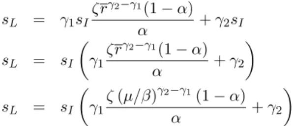
factor, β, is calibrated to be 0.99, which is equivalent to an annual steady state real interest rate of 4 percent. Following Goodfriend and McCallum (2007) we set the annual banking spread at steady state to 2 percentage points or µ = 1.005. The depreciation rate, δ, is set equal to 0.05 per quarter. We set α = 0.36 which roughly implies a steady state share of labour income in total output of 65%. The share of steady state consumption (sc) is set equal to 0.725, while
the share of steady state investment (sI) is set equal to 0.275. Using the credit
market clearing condition we show the relationship between the share of loans and investment at the steady state. Parameters γ1, γ2regulate the importance of
labour and investment cost channels; we set γ1,2= 1, implying full-cost channel.
Finally, we set the value of the Calvo parameter ω (fraction of firms which do not adjust their prices) as equal to 0.66 consistent with the findings reported in Gali and Gertler (1999).
4.
Banking spread and the propagation of shocks
In our model the strength of the firm-bank relationship is represented by the size of the variable θ. High θ implies a firm is more attached to the set of banks that have offered them loans in the past, making the demand for loans less interest rate elastic, increasing the market power of banks. On the other hand, in order to maintain a relationship, preventing the firm from searching for other credit houses, the bank must refrain from changing spreads sharply. That can be interpreted as a cost for the bank as it develops these relationships. Parameter ψ controls this cost. In fact ψ is also important to ensure our model economy has a unique equilibrium since a high volatility of banking spreads under strong lending relationships may imply the economy does not converge back to equilibrium after a shock. The determinacy properties of our model are discussed in detail in the next section.
Given that very little empirical research has been done on banking spreads, we do not have a specific measure to calibrate θ and ψ. In view of that we focus on the qualitative responses as θ increases from zero to 0.75. Additionally, we set ψ = 256. In order to facilitate the comparison of our impulse response to 6In order to establish how much spread persistence that entails we have run spread responses
after an inflation shock, holding θ = 0.45, for ψ = 0 and ψ = 25. With higher ψ, spreads do not increase as much but are more persistent, although the half-live in both cases is still only one period. After four periods, the spread deviations converge. In the first case the ratio of the standard deviation of spread and GDP is 1.4%, while in the second it decreases to 0.8%.
ones presented in other studies (e.g. Woodford (2003) and Curdia and Woodford (2008)) we set the Taylor rule parameters as follows: ²π = 2, ²y = 0.5 and ²r = 0.
The qualitative answers do not change when other parameter configurations are considered7. We first look at the economy’s response to four standard types of
shocks: a taste shock directly associated with the consumption Euler equation, an investment shock, that reflects an unexpected boost in investment, an infla-tion (or supply) shock associated with the New Keynesian Phillips Curve and finally a policy shock to the Taylor Rule. The vector of shocks is defined as ξt= [εc,t, εI,t, επ,t, εr,t]0. All four shock processes are assumed to have an
autocor-relation coefficient equal to 0.75; their standard deviations are set equal to 1%. Given that our model explicitly includes a banking sector we can also consider a financial sector shock that can be interpreted as a banking capital shock or temporary change to bank regulation that affects the bank loan rate decision. We start the analysis by looking at the cyclical properties of banking spreads. 4.1 Banking spread cyclical properties
Aliaga-Diaz and Olivero (2007) find evidence in support of the countercycli-cality of banking spreads (or as they refer to, price-cost margin) using data on the United States banking sector for the period 1984-2005. One of the theoretical rationalizations of variations to banking spread impacting the real economy is given by Bernanke, Gertler, and Gilchrist (1999), based on a costly state verifi-cation set-up. However, as that empirical result holds after controlling for credit risk, monetary policy and the term structure of interest rates, there are other factors driving the cyclical properties of spreads. We investigate whether lend-ing relationships, which increase the market power of banks, can also rationalize countercyclical banking spreads.
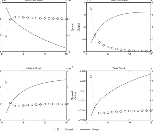
Figure 1 shows the output and banking spread responses to our four main shocks. After a demand shock (investment shock), output increases, while the banking spread decreases. This is consistent to the view that banks take advan-tage of period of relatively high output to build relationships, decreasing markups to attract firms, since they recognize that the current rate decision affects future loan demand.
On the other hand, after a cost push shock, output decreases and interest rate margins increase. When output decreases, banks take advantage of the relationships already built and the fact that firms will have more difficulties to
Figure 1: Cyclical Properties of Banking Spread - θ = 0.75, ψ = 25 0 5 10 15 4 6 8 10 x 10−3 Output Investment Shock 0 5 10 15 −2 −1 0 1 x 10⁻³ Spread 0 5 10 15 −15 −10 −5 0 5 x 10⁻⁴ Output
Taylor Rule Shock
0 5 10 15 0 0.5 1 1.5 2 x 10⁻⁴ Spread 0 5 10 15 −0.03 −0.02 −0.01 0 Output Inflation Shock 0 5 10 15 −2 0 2 4 x 10⁻³ Spread 0 5 10 15 −0.016 −0.014 −0.012 −0.01 −0.008 −0.006 Output Taste Shock 0 5 10 15 −5 0 5 10 15 20 x 10−4 Spread Spread | Output
acquire funds, increasing the banking spread. The first to identify the firm’s cost of entering into a credit relationship was Rajan (1992). This bank practice of exploiting lending relationship is verified empirically by Schenone (2009) and Santos and Winton (2008). The latter, using firm level data in the United States, finds that firms without access to corporate bond market face banking spread increases of up to 95 basis points in a recession, while for firms with bond market access, th spread can increase up to 28 basis points. In Europe, where firm-bank relationships are more common these numbers could be even greater. In our simulation, after a cost push shock, spreads increased by roughly 110 basis points (annualized or 30 in the quarter). We also find countercyclical spreads after both a taste (Euler equation) and a contractionary monetary policy (Taylor Rule Shock). In both cases, output decreases and banks once again exploit credit relationships increasing the spread.
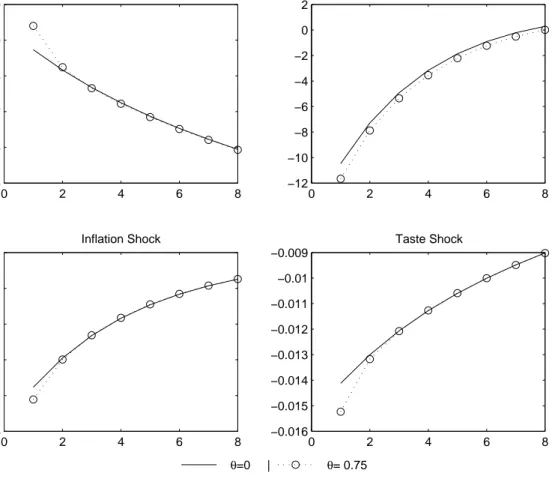
4.2 Endogenous spread, output responses and monetary policy In order to identify the impact of lending relationships and the endogenous spread movements it generates onto the main variables of the economy we com-pare the impulse responses of a model with constant spread, setting θ = ψ = 0, and our benchmark model with θ = 0.75 and ψ = 25. We firstly look at output responses. Spread movements amplify output responses to all shocks (figure 2). Under a model with constant banking spread, output decreases after a standard cost push shock. However, if banks try to exploit credit relationships, increas-ing spreads, output will decrease even further. Higher loan rates imply a direct increase on the cost of hiring labour and investing in capital. That leads to a further decrease in investment and labour demand, leading to lower output levels.
Figure 2: Endogenous Spread and Amplification of Output Responses
0 2 4 6 8 5 6 7 8 9 10x 10 −3 Investment Shock 0 2 4 6 8 −12 −10 −8 −6 −4 −2 0 2x 10
−4 Taylor Rule Shock
0 2 4 6 8 −0.03 −0.025 −0.02 −0.015 −0.01 −0.005 Inflation Shock 0 2 4 6 8 −0.016 −0.015 −0.014 −0.013 −0.012 −0.011 −0.01 −0.009 Taste Shock θ=0 | θ= 0.75
initial rise in output. Banks take advantage of higher demand for credit to de-crease spreads, attempting to build as many relationships as possible. Decreasing spreads imply lower labour and investment costs, boosting production.
After a contractionary monetary shock output remains below its shadow level under constant spreads for a greater number of periods. Spread movements are more persistent in this case, pushing output further down. In the case of invest-ment, inflation and taste shocks, spreads quickly move back close to zero, thus output converges to its shadow level after a few periods8.
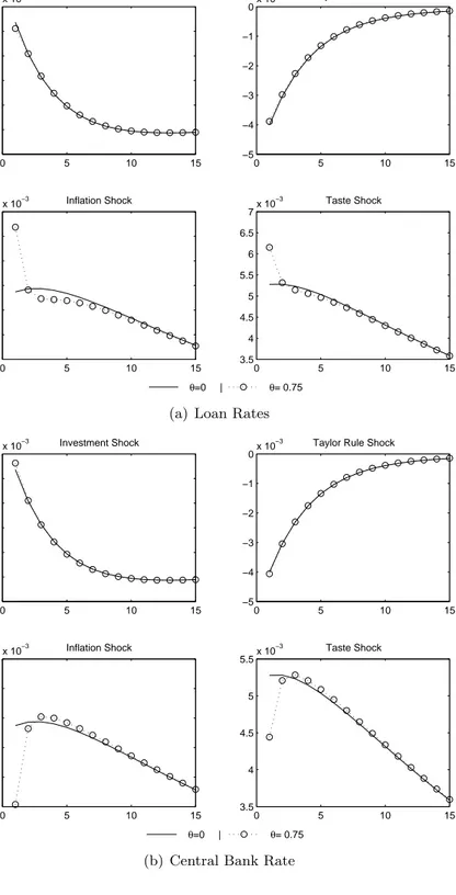
The amplification of output responses due to changes in banking spreads ob-served here is similar to the one initially proposed by Bernanke, Gertler, and Gilchrist (1999), although the channel through which it impacts the economy is quite different. In our model loan rates directly impacts the firm’s costs of pro-duction. As a result of that, as banks use their market power, moving spreads countercyclically to maximize profits, they reinforce the production costs move-ments after a shock, leading to greater output responses. Figure 3 (a) shows the banking loan rate movement after the shocks for θ = 0 and 0.75. As expected, as banking spreads move, so does the loan rates. However, spread deviations are always greater than the actual difference between the loan rates when comparing the θ = 0 and 0.75 cases. For instance, while spreads increase by roughly 30 basis points (by quarter) after an inflation shock, the net difference of loan rate devi-ations only increase by roughly 15 basis points. The remaining 15 basis points is covered by an active monetary policy that does react (indirectly) to banking spread movements.
Figure 3 (b) shows how the base interest rate RCB set by the central bank
responds to our four main shocks. As it is clear, when spreads increase (in relation to its shadow level under constant spreads) after the shock, the central bank rate moves in the opposite direction (again in relation to its movement when θ = 0), offsetting some of the impact on the loan rates faced by firms and dampening the potential effect of endogenous banking spreads on the real economy. In the case of an inflation shock, the central bank interest rate is 15 basis points lower than it would have been under constant spreads. Effectively, an increase in spreads results in an endogenous tightening of monetary conditions, forcing the central bank to adjust the base rate accordingly. Nonetheless, as we have seen, output responses are still amplified, hence despite the fact that monetary policy actively
8We conjecture that altering X
tto link Lt,i,jto Lt−1,i,j(see footnote 2) would generate more
persistent spread movements since in order to form relationships banks must offer firms a path of future rates and not only the current rate.
Figure 3: Endogenous Spread and Interest Rate Response 0 5 10 15 −4 −2 0 2 4 6 8x 10 −3 Investment Shock 0 5 10 15 −5 −4 −3 −2 −1 0x 10
−3 Taylor Rule Shock
0 5 10 15 2.5 3 3.5 4 4.5 5 5.5x 10 −3 Inflation Shock 0 5 10 15 3.5 4 4.5 5 5.5 6 6.5 7x 10 −3 Taste Shock θ=0 | θ= 0.75
(a) Loan Rates
0 5 10 15 −4 −2 0 2 4 6 8x 10 −3 Investment Shock 0 5 10 15 −5 −4 −3 −2 −1 0x 10
−3 Taylor Rule Shock
0 5 10 15 2.5 3 3.5 4 4.5 5x 10 −3 Inflation Shock 0 5 10 15 3.5 4 4.5 5 5.5x 10 −3 Taste Shock θ=0 | θ= 0.75
moves trying to offset spread movements, it can not do so completely and the increase in loan rates lead to more volatile output responses. Inflation, however, does not change as much, following a similar path in both cases, thus the change in monetary policy does not generate increasing inflationary pressure (See figure 8 in the Appendix).
Two important aspects of this result should be highlighted. Firstly, the base interest rate (or monetary policy instance), responds quite differently to shocks depending on whether lending relationships are in place or not. Thus, if the cen-tral bank is uncertain whether these relationships are strong or not, or uncertain about the true model of the economy, it may set an incorrect interest rate path, failing to stabilize output gap and inflation. De Fiore and Tristani (2008) obtain a similar conclusion while looking at a monetary policy that tracks the natural rate in a model with and without credit frictions. Their model incorporates the financial accelerator into a standard New Keynesian model and they find that credit frictions imply different natural rate dynamics and hence different mon-etary policy responses to the shocks impacting the economy. Once again, the results are similar though the channel is different, while spread here moves due to firm-bank relationship, in De Fiore and Tristani (2008) it moves due to changes in the firm’s net worth.
Secondly, there is a general view that as banking spreads move, monetary pol-icy should immediately adjust reducing the interest rate, since a higher spread would imply monetary conditions are tighter than what the original policy in-tended. In our benchmark model we consider a standard Taylor rule whereby the base rate only responds to output gap and inflation deviations, thus this immediate adjustment is not in place. Nonetheless, based on the simulations results presented here, as spread changes do have an effect on the output and inflation responses to the shocks impacting the economy, we find that the base rate indirectly responds to spread movements. This response, however, is not a one-to-one adjustment.
Given that at this stage we do not look at optimal monetary policy and although the standard Taylor rule implies monetary policy adjusts to spread movements, one should still verify if impulse responses change significantly when other monetary policy rules are considered. In the next section we look at two types of alternative policies, one that augments the original Taylor rule with credit aggregates and one with banking spreads.
4.3 Alternative Monetary Policy rules
Taylor (2008) advocates that the central bank base rate should respond not only to output gap and inflation deviations but also to changes in the banking spread. Such framework allows the central bank to accommodate the monetary policy to changes in the banking/financial sector conditions, generating the ap-propriate interest rate to stabilize the impact of shocks hitting the economy. This adjusted Taylor rule takes into consideration that there is not only one interest rate type that is important for the transmission of monetary policy, making the monetary rule to account for movements in both rates, the base rate, which impact the consumption decision through the standard Euler equation and the loan rate, which impact production and investment costs. Formally, the spread-adjusted Taylor Rule is given by:
b
rt,CB= ²ybyt+ ²ππbt+ ²rrbt−1,CB− ²µµbt,
For 0 < ²µ < 1, the central bank effectively targets a hybrid rate that is a weighted average of the loan rate and the base interest rate. If ²µ= 1, then the
central bank in fact targets the loan rate instead of the base interest rate in the economy. We present the results for ²µ= 0.5 and ²µ= 1 while keeping the other Taylor rule parameters unchanged (²π = 2, ²y = 0.5 and ²r= 0). Figure 4 shows
impulse responses after an exogenous supply and demand shock.
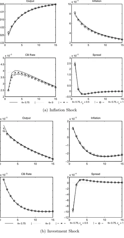
When the monetary policy responds to banking spread changes, the previously observed output amplification is offset. After an inflation shock, the central bank base rate does not increase as much as when the original Taylor Rule is considered such that the output decrease is actually smaller than when spreads are constant. Note that in the case of the inflation shock, the smaller output deviation is not “paid” by more inflation pressures. Although inflation initially increases more, it is less persistent, falling down faster to its steady state level.
After an investment shock, output does not increase as much as when a basic Taylor rule is considered, so a monetary policy that adjusts to spread movements is able to offset the cost channel impact of lower banking spreads. The adjusted Taylor rule also deliver lower initial inflation response, although now the infla-tion response is flatter. Note, however, that after an investment shock inflainfla-tion deviation is initially positive but after the fifth period it becomes negative and converges to zero from below, hence, under this policy rule, inflation also
con-Figure 4: Spread-Adjusted Taylor Rule 0 5 10 15 −0.03 −0.025 −0.02 −0.015 −0.01 −0.005 Output 0 5 10 15 2 4 6 8 10x 10 −3 Inflation 0 5 10 15 2 2.5 3 3.5 4 4.5 5x 10 −3 CB Rate 0 5 10 15 −0.5 0 0.5 1 1.5 2 2.5 3x 10 −3 Spread θ= 0.75 | θ= 0 | θ= 0.75, εµ = 0.5 | θ= 0.75, εµ = 1
(a) Inflation Shock
0 5 10 15 4 5 6 7 8 9 10x 10 −3 Output 0 5 10 15 −3 −2 −1 0 1 2x 10 −3 Inflation 0 5 10 15 −4 −2 0 2 4 6 8x 10 −3 CB Rate 0 5 10 15 −12 −10 −8 −6 −4 −2 0 2x 10 −4 Spread θ= 0.75 | θ= 0 | θ= 0.75, εµ = 0.5 | θ= 0.75, εµ = 1 (b) Investment Shock
verges more rapidly to its steady state value. Therefore, there is indication that although under a standard Taylor rule monetary policy implicitly respond to banking spread movements, adjusting the monetary rule to explicitly include a term dependent on the spread may improve the stabilization of shocks.
Christiano, Motto, and Rostagno (2007) present a model that include financial variables and nominal lending contracts and argue that including a measure of broad money into a standard Taylor rule result in lower GDP volatility. Based on these finding we also consider the changes to the main impulse responses after a supply and demand shock assuming monetary policy is set according to a credit-adjusted Taylor rule that includes an additional term dependent on real credit aggregates. Formally, the rule is given by:
b
rt,CB = ²yybt+ ²ππbt+ ²rbrt−1,CB+ ²lblt,
where ²y = 0.5, ²y = 2 and ²r= 0.5.
Given the assumption of full cost channel, credit aggregates deviations are closely related to deviations in output. Hence, increasing ²lfrom zero to 0.4 leads
to similar changes as if the parameter on output had increased (see figure 10 in the Appendix). After a supply shock, output does not decrease as much, but inflation increases substantially more than in the case of the standard Taylor rule. After a demand shock, output does not increase as much, but inflation drops considerably more. Note that, as we increase ²l, holding ²y constant, indeterminacy obtains.
In order to avoid this we increase ²r from zero to 0.5 (see Aksoy, Basso, and Coto-Martinez (2009) for a detailed discussion of indeterminacy due to the cost channel of monetary policy).
4.4 Banking/Financial Shock
Our model considers a type of financial sector friction due to the develop-ment of lending relationships. As we explicitly model the banking sector we can consider an alternative shock, interpreted as a banking capital shock or tempo-rary change in bank regulations, that impact the bank’s loan rate setting decision (equation (26j)). That leads to an increase in spread and a decrease in investment and output. Consumption increases pushing inflation slightly up. Modifying the monetary policy, setting the base rate using a spread-adjusted Taylor rule does not seem to generate improved stabilization of output and inflation. If the shock is not persistent, responding to spreads may reduce the output contraction but
it creates additional inflationary pressures.
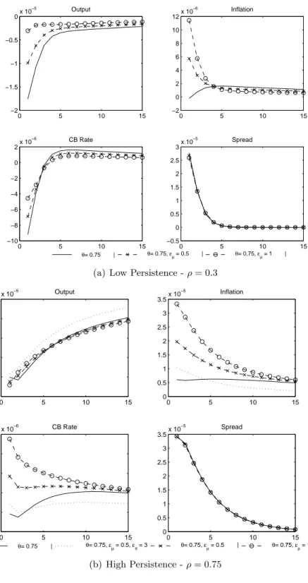
Targeting spread movements in this case is similar to the central bank becom-ing more concerned with output deviations than inflation deviations. Given the forward looking nature of the inflationary process, the initial drive to decrease the base rate as spread increases leads to high inflationary pressures. Taking that into account actually means that the base rate does not decrease as much as in the case when monetary policy is set based on the standard Taylor Rule. If shocks are very persistent, this forward looking element is very strong such that as the central bank takes the banking spread into consideration to set policy it delivers a high inflation rate but equivalent output deviations. Figure 5 shows the impulse responses for both cases, when shocks have low persistence (ρ = 0.3) and high persistence (ρ = 0.75). A similar result obtains when a credit-adjusted Taylor rule is considered.
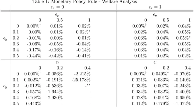
4.5 Monetary Policy Rules and Welfare
Spread-adjusted Taylor rules seem to perform better that standard Taylor rules in stabilizing both supply and demand shocks. Targeting credit aggregate is less successful. In view of that we employ Schmitt-Grohe and Uribe (2004a) methodology to quantify the welfare costs of alternative policy rules testing if indeed spread-adjusted Taylor rules lead to higher (conditional) welfare. To this end we write the non-linear equilibrium conditions in the following format:
Et(yt+1, yt, xt+1, xt) = 0
where yt contains the non-predetermined variables of the model and xt
con-tains the endogenous predetermined variable (x1t) and the exogenous shocks (x2t). Given our interest on policy rules we exclude the Taylor rule shock and set x2
t = [εc,t, εI,t, επ,t, εb,t]0, where the last is the banking sector shock.
Further-more we assume that:
x2t+1 = Λx2t+ eκeΘzt,
where Λ determines the persistence of the shocks, eκe the standard deviation of
shocks9, Θ scales standard deviations and z
t is an iid shock. The economy’s
welfare is given by the household’s conditional expectation of lifetime utility V0,
given by:
Figure 5: Banking Shock 0 5 10 15 −2 −1.5 −1 −0.5 0x 10 −5 Output 0 5 10 15 −2 0 2 4 6 8 10 12x 10 −6 Inflation 0 5 10 15 −10 −8 −6 −4 −2 0 2x 10 −6 CB Rate 0 5 10 15 −0.5 0 0.5 1 1.5 2 2.5 3x 10 −5 Spread θ= 0.75 | θ= 0.75, εµ = 0.5 | θ= 0.75, εµ = 1 |
(a) Low Persistence - ρ = 0.3
0 5 10 15 −3 −2.5 −2 −1.5 −1 −0.5x 10 −5 Output 0 5 10 15 0 0.5 1 1.5 2 2.5 3 3.5x 10 −5 Inflation 0 5 10 15 −5 0 5 10 15 20x 10 −6 CB Rate 0 5 10 15 0 0.5 1 1.5 2 2.5 3 3.5x 10 −5 Spread θ= 0.75 | θ= 0.75, εµ = 0.5, επ = 3 θ= 0.75, εµ = 0.5 | θ= 0.75, εµ = 1 | (b) High Persistence - ρ = 0.75
V0 = Et ∞ X t=0 βt à Ct1−σ 1 − σ − χ Ht1+η 1 + η !
Including V0as one of the variables in the vector yt, the solution to the system
is given by yt= g(xt, Θ) and xt+1= h(xt, Θ) + κeΘzt. Finally, the non-stochastic steady state is given by xt= x and Θ = 0.
As in Schmitt-Grohe and Uribe (2004a) we define the welfare cost of adopting an alternative policy regimes a compared to a policy regime r as a portion of consumption W C such that the household would be indifferent between the two policies. Formally: Vra= Et ∞ X t=0 βt µ (Ca t)1−σ 1 − σ − χ (Ha t)1+η 1 + η ¶ = Et ∞ X t=0 βt µ ((1 − W C)Cr t)1−σ 1 − σ − χ (Hr t)1+η 1 + η ¶
Then, using the fact that the first derivative of the policy function g with respect to Θ evaluated at the steady state (xt = x and Θ = 0) is zero (see
Schmitt-Grohe and Uribe (2004b)), the welfare cost can be approximated to:
Welfare Cost = W C(x, 0) = −(1 − β) · ∂2Va ∂Θ∂Θ ¯ ¯ ¯ (x,0)− ∂2Vr ∂Θ∂Θ ¯ ¯ ¯ (x,0) ¸ Θ2 2 We present a model with cost channels of monetary policy, in which, con-trary to standard New Keynesian models, policy makers face a trade-off between stabilizing the inflation rate and stabilizing the output gap (see the discussion in Ravenna and Walsh (2006)), creating a policy bias towards more aggressive inflation stabilization. As our focus is on the welfare impact of including addi-tional terms dependent on credit market measures we fix the value of ²π = 2 and
measure welfare changes by varying other policy rule parameters10, therefore:
b
rt,CB = 2bπt+ ²ybyt+ ²rrbt−1,CB− ²µµbt
b
rt,CB = 2bπt+ ²ybyt+ ²rrbt−1,CB+ ²lblt.
Table 1 shows the welfare costs (W C) for different policy parameter combi-nations. We set the reference policy, for which W C = 0, to be the first point
10We also run simulations for lower and higher values of ²
π. The conclusions of the welfare
Table 1: Monetary Policy Rule - Welfare Analysis ²r = 0 ²r = 1 ²µ ²µ 0 0.5 1 0 0.5 1 0 0.00%† 0.01% 0.02% 0.00%† 0.02% 0.04% 0.1 0.00% 0.01% 0.02%∗ 0.02% 0.04% 0.05% ²y 0.2 -0.01% 0.00% 0.01% 0.03% 0.04% 0.05%∗ 0.3 -0.06% -0.05% -0.04% 0.03% 0.04% 0.05% 0.4 -0.17% -0.16% -0.14% 0.03% 0.04% 0.04% 0.5 -0.44% -0.42% -0.41% 0.01% 0.02% 0.02% ²l ²l 0 0.2 0.4 0 0.2 0.4 0 0.000%† -0.056% -2.215% 0.000%† 0.049%∗ -0.070% 0.1 0.002%∗ -0.191% -25.178% 0.021% 0.033% -0.140% ²y 0.2 -0.012% -0.536% -∗∗ 0.032% 0.007% -0.243% 0.3 -0.057% -1.644% - 0.034% -0.032% -0.400% 0.4 -0.168% -7.930% - 0.028% -0.091% -0.650% 0.5 -0.443% - - 0.012% -0.179% -1.072%
† Indicates the reference policy for that quadrant
∗ Indicates the best set of policy parameters for that quadrant
∗∗ A dash indicates there was no unique equilibrium for these policy parameters.
in each quadrant, where ²µ =²y=²l= 0. For each degree of response to output deviations (²y), increasing ²µ, the response to banking spread changes, leads to
an increase in welfare (welfare costs are always increasing in each row for the two top quadrants). The welfare analysis presented here points to the conclusion that the central bank, in order to maximize welfare, should target the loan rate, setting ²µ= 1, rather than the central bank base rate (²µ= 0) or the average of
the two rates (²µ = 0.5). Lending relationships introduce a dynamic distortion
in credit markets, since it gives the banks incentives to vary spreads moving the economy further away from steady state. When the base rate responds directly to spread movements, the central bank is able to partially offset this distortion, increasing welfare.
The same result is not observed when credit aggregates are targeted. The only case where it is optimal to target credit aggregates is when the policy rule is set with inertia. In this case credit aggregates replace output targeting being a more efficient choice to maximize welfare.
5.
(In)Determinacy Analysis
We now turn to the analysis of the implications of strengthening firm-bank relationships to the determinacy properties of our model economy. We first con-sider an economy where banks do not face spread adjustment costs, being free to exploit lending relationships already formed. Consequently we set ψ = 0.
5.1 (In)Determinacy in the Model without Adjustment Costs
As it is well known the policymaker using Taylor-type rules to stabilize infla-tion and output gap may be a source of instability if it does not select appropriate reaction coefficients for the monetary rule. To provide a comprehensive discus-sion we consider not only the standard Taylor rule that targets output gap and inflation but the two alternative rules discussed in the previous section, whereby the central bank also responds directly to changes in banking spreads and credit aggregates.
We show that the range of policy rules support three possible outcomes: i) a unique solution ii) multiple equilibria (sun spots) and iii) no solution. Of course, our interest is to determine the policy rules that deliver a unique solution. We will first concentrate on the standard Taylor rule where the main policy parameter of interest are ²π, ²y and ²r.
5.1.1 Simple Monetary Rules
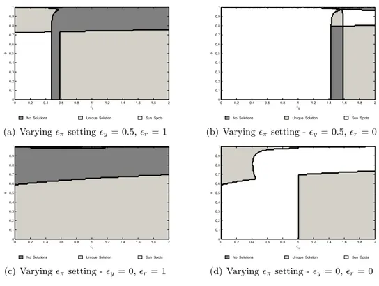
In figure (6) we report the determinacy areas for different (fixed) values of ²y
and ²r, when ²π changes from 0 to 2 and when θ, the parameter that governs the
strength of firm-bank relationships in the economy, change from zero to 1. The dark grey shaded areas show the no solution cases, the light grey the region where the model delivers a unique solution and the white shows the multiple equilibria cases.
Firstly, we present in Figure 6(a) the case when the central bank targets output gap (²y = 0.5) and past interest rates (²r = 1). We observe that all
three solutions are possible depending on the parameter values. Unique solution obtains when θ is lower than 0.7 and when the inflation coefficient is greater than 0.6.
As expected (see the conclusions of our previous work Aksoy, Basso, and Coto-Martinez (2009)), if interest rate smoothing is not present (figure 6(b)) the
Figure 6: Indeterminacy Analysis - Effect of Firm-Bank Relationship επ θ 0 0.2 0.4 0.6 0.8 1 1.2 1.4 1.6 1.8 2 0 0.1 0.2 0.3 0.4 0.5 0.6 0.7 0.8 0.9 1
No Solutions Unique Solution Sun Spots
(a) Varying ²π setting ²y= 0.5, ²r = 1
επ θ 0 0.2 0.4 0.6 0.8 1 1.2 1.4 1.6 1.8 2 0 0.1 0.2 0.3 0.4 0.5 0.6 0.7 0.8 0.9 1
No Solutions Unique Solution Sun Spots
(b) Varying ²πsetting - ²y= 0.5, ²r = 0 επ θ 0 0.2 0.4 0.6 0.8 1 1.2 1.4 1.6 1.8 2 0 0.1 0.2 0.3 0.4 0.5 0.6 0.7 0.8 0.9 1
No Solutions Unique Solution Sun Spots
(c) Varying ²πsetting - ²y= 0, ²r = 1 επ θ 0 0.2 0.4 0.6 0.8 1 1.2 1.4 1.6 1.8 2 0 0.1 0.2 0.3 0.4 0.5 0.6 0.7 0.8 0.9 1
No Solutions Unique Solution Sun Spots
(d) Varying ²πsetting - ²y= 0, ²r = 0
central bank needs to be more aggressive towards inflation deviation to guaran-tee determinacy but the conclusions regarding the impact of changing θ remain unchanged. Note that the areas of stability dictated by the model are somewhat different than those suggested by the Taylor-Woodford principle, in which by set-ting the inflation coefficient greater than 1 a policymaker, who also targets output gap and smooths interest rates, is able to ensure the stability of the economy.
The (in)determinacy regions when the model includes no output gap target in the policy rule (²y = 0) yet retains interest rate smoothing is presented in
figure 6(c). There is a unique solution to the model for low θ irrespective of the size of the inflation coefficient in the Taylor rule. This is an unusual result as it implies that the model delivers a unique equilibrium even if the policymaker is not concerned with inflation and output gap at all and if it just follows a interest rate smoothing policy.
In figure 6(d) we present the case where the policymaker is only concerned about inflation (²y = 0 and ²r = 0). When the firms intrinsic link to banks they
dealt in the previous period is relatively weak (0 < θ < 0.6) policymaker ensures stability when the inflation coefficient (²π) is greater than 1.
In all four cases, when the central bank cares about inflation deviations a value of θ greater than around 0.8 (sometimes lower) implies our economy does not con-verge back to the steady state equilibrium after a shock, or our rational expecta-tions model has either no or many soluexpecta-tions. If there are no spread adjustment costs, and lending relationships are strong then banking spreads are very volatile. As we have seen, spread changes directly impact output and loan demand, which in turn fuel another round of spread adjustment, leading to output-loan spirals. This result is directly linked to the significant portion of loan demand that is not interest rate sensitive11. If interest rate inertia is present, then the economy
diverges. Otherwise, our model delivers multiplicity of equilibria. On the other hand, for a higher level of θ an aggressive stand against inflation is destabilizing; in fact only when the central bank reacts very modestly to inflation (0 < ²π < 0.4)
a unique equilibrium exists, in stark contrast to the existing literature.
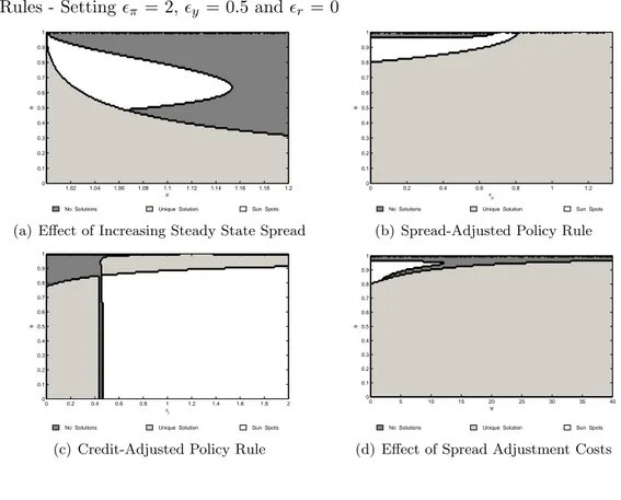
Finally, figure 7(a) shows the effect of increasing θ and the steady state bank-ing markup u. We initially set u = 1.005 implybank-ing an annual bankbank-ing spread of 2 percentage points base on a model calibrated for the U.S.. However in some economies where competition in the banking sector is weaker this number can be considerably higher. Higher steady state spread levels imply that indetermi-nacy occur for lower levels of θ. Thus, indetermiindetermi-nacy problems are worsened in economies with strong firm-bank relationships associated with high average spread levels.
We conclude that active policymaking under lending relationships and en-dogenous banking spreads significantly alters stability conditions as compared to three equation New Keynesian model. While interest rate smoothing is impor-tant for stability purposes, there is a much less clear-cut case for targeting output gap. One key result of Taylor-Woodford work is that in setting the short term rates policymaker needs to respond more than one to inflation changes. Here we document that is not necessarily the case. Finally, the strength of firm-bank re-lationships turns out to be crucial in the determinacy discussion. Strong lending relationships imply less stable economies forcing the central bank to change the policy rule. In the previous section we showed that policy rules that respond to credit conditions may generate improved stabilization of shocks and higher condi-tional welfare levels. In the next section we verify if these alternative policy rules also circumvent some of the indeterminacy problems related to strong lending
11Note that this is similar to the price indeterminacy problem observed in the framework
relationships.
Figure 7: Indeterminacy Analysis - Adjustment Costs and Alternative Policy Rules - Setting ²π = 2, ²y = 0.5 and ²r = 0
µ θ 1.02 1.04 1.06 1.08 1.1 1.12 1.14 1.16 1.18 1.2 0 0.1 0.2 0.3 0.4 0.5 0.6 0.7 0.8 0.9 1
No Solutions Unique Solution Sun Spots
(a) Effect of Increasing Steady State Spread
εµ θ 0 0.2 0.4 0.6 0.8 1 1.2 0 0.1 0.2 0.3 0.4 0.5 0.6 0.7 0.8 0.9 1
No Solutions Unique Solution Sun Spots
(b) Spread-Adjusted Policy Rule
εl θ 0 0.2 0.4 0.6 0.8 1 1.2 1.4 1.6 1.8 2 0 0.1 0.2 0.3 0.4 0.5 0.6 0.7 0.8 0.9 1
No Solutions Unique Solution Sun Spots
(c) Credit-Adjusted Policy Rule
ψ θ 0 5 10 15 20 25 30 35 40 0 0.1 0.2 0.3 0.4 0.5 0.6 0.7 0.8 0.9 1
No Solutions Unique Solution Sun Spots
(d) Effect of Spread Adjustment Costs
5.1.2 Alternative Monetary Policy Rules
Instead of inflation and output gap targeting only, the policymaker may also target the spread between the actual bank rate and the policy rate next to key fundamentals. As we have shown the monetary rule in this case takes the follow-ing form:
b
rt,CB = ²yybt+ ²πbπt+ ²rbrt−1CB− ²µµ.b
This targeting rule may be particularly appealing under our set-up with bank distortions represented by the strength of lending relationships(θ) when no ad-justment costs are in place. If the central bank base rate responds directly to spread changes, the final loan rates will not be as volatile as spreads. As a result of that loan demand will not move as sharply, breaking the spread-output spiral that lead to indeterminacy of rational expectations equilibrium in our model. As figure 7(b) shows targeting spread movement does indeed improve the
perfor-mance of the model in terms of stability.
The other alternative monetary policy rule considered in the previous section includes a direct term depend on credit aggregates. Figure 7(c) shows the results. In this case the modified policy rule does not ameliorate the indeterminacy prob-lem. As discussed before targeting credit aggregates is very similar to increasing the importance of output movements relative to inflation deviation. Confirm-ing the results in the literature, excess output concern implies multiplicity of equilibria.
5.2 (In)Determinacy in the Model with Adjustment Costs
Finally, we briefly evaluate the determinacy properties of our benchmark model with adjustment costs. Figure 7(d) shows that modifying the basic banking model with banking spread adjustment costs improves the determinacy perfor-mance of the model as compared to the model without adjustment costs. As we increase ψ, the parameter that controls the size of the adjustment cost, the range for which our model delivers a unique solution also increases. These results are robust to changing Taylor rule parameters (²y, ²r and ²π ) and to alternative
targeting regimes such as spread targeting and loan targeting.
6.
Conclusions
We present a simple staggered price DSGE model that incorporates a basic and relevant feature of financial intermediation, namely, lending or firm-bank relationships. While such a relationship benefits firms through the reduction of information asymmetries they also create hold-up costs; firms become locked to a bank, reducing their bargaining power over credit rates. Empirical estimates presented by Santos and Winton (2008) indicate that during recessions firms that are locked into relationships have their borrowing costs increased by as much as 95 basis points.
Our results show that banking spreads move in the opposite direction to output, reinforcing production costs movements after a shock. Banks decrease spreads attempting to form as many relationships as possible during booms and increase spreads to sustain profitability during recessions, exploiting the firms locked into pre-existing relationships. Due to the cost channel of monetary trans-mission, countercyclical spreads lead to amplification of output responses. The