An Analysis of the Telecommunications Business in China by Linear Regression

(1)

An Analysis of the Telecommunications

Business in China by Linear Regression

Authors:

Ajmal Khan

h09ajmkh@du.se

Yang Han

v09yanha@du.se

Supervisor:

Dao Li

dal@du.se

C-level in Statistics, January 2010

School of Technology and Business Studies

Högskolan Dalarna, Sweden

(2)

Dalarna University Tel. +46(0)237780000

Röda Vägen 3S-781-88 Fax:+46(0)23778080

Borlänge Sweden http://du.se

1

Abstract

In this paper, we study the influence of the National Telecom Business Volume by the data in 2008 that have been published in China Statistical Yearbook of Statistics. We illustrate the procedure of modeling “National Telecom Business Volume” on the following eight variables, GDP, Consumption Levels, Retail Sales of Social Consumer Goods Total Renovation Investment, the Local Telephone Exchange Capacity, Mobile Telephone Exchange Capacity, Mobile Phone End Users, and the Local Telephone End Users. The testing of heteroscedasticity and multicollinearity for model evaluation is included. We also consider AIC and BIC criterion to select independent variables, and conclude the result of the factors which are the optimal regression model for the amount of telecommunications business and the relation between independent variables and dependent variable. Based on the final results, we propose several recommendations about how to improve telecommunication services and promote the economic development.

(3)

Röda Vägen 3S-781-88 Fax:+46(0)23778080

2

1 Introduction

1.1 Background

With gradually developing of reform policy according to the national economy, the Chinese government has adjusted significantly for the policy of telecommunications industry to make its telecommunications industry to develop stably and rapidly. As the telecommunications industry is related to the national people's livelihood and it is also an important industry in the economy, the role and impact of promoting the economics are self-evident. In the past two decades, China's telecommunications industry has grown out of imaging. Especially after July 2001 when the fee of phone initial installation and mobile telephone network access were cancelled in China, the growth rate of total revenue of telecommunications industry has been accelerated. The volume of post and telecommunications business in 2001 achieved 406.97 billion Yuan, which is 24% more than the volume in the last year 2000; the aggregate telecommunications reached 361.2 billion Yuan that grew about 25%. For example, the capacity of Office Telephone Exchanges went to 199.764 million with cumulatively growing 20.914 million in a whole year; the capacity of mobile communication exchange had 221.202 million, cumulatively grown 90.637 million in a whole year; the account of fixed telephone subscribers gained 179.034 million, cumulative growth of 34.830 million; the account of mobile phone users increased to 59.546 million. These data show that China becomes one of the largest mobile communications power in the world.

The telecommunications industry is related to people's livelihood, and it is the major industry to promote the economic growth. The analysis for the development factors of the telecommunications industry holds great significance for how to speed up the future development of the telecommunications industry, and it also reveal the laws of economic operation. This is very important for the national economy stable and rapid development.

(5)

Röda Vägen 3S-781-88 Fax:+46(0)23778080

4

2 Data

According to the relevant information, we are interested the following variables which are mostly concerned as factors of the aggregate telecommunications. Those variables are: GDP, the level of household consumption, total retail sales of social commodities consumption, renovation investment, the local telephone exchange capacity, mobile telephone exchange capacity, the amount of the end of mobile phone users, and local telephone end users (See Appendix for variable descriptions in details).

This essay try to establish a linear regression model of the aggregate telecommunications based on those variables, then we do the model selection by some basic principles in this topic such as AIC, BIC criteria etc..

2.1 Individual Variable Descriptions

2.1.1 Total changes in China Telecom's business

In our data, aggregate telecommunications has accumulated 2243.95 billion Yuan in 2008, 21.0% increasing from 2007. Telecommunications on business income is 813.99 billion Yuan with growing 7.0%. Telecommunications investment in fixed assets achieves 295.37 billion Yuan with growing 29.6%. Telecom value-added accomplishes 472.62 billion Yuan which increases 0.3%.

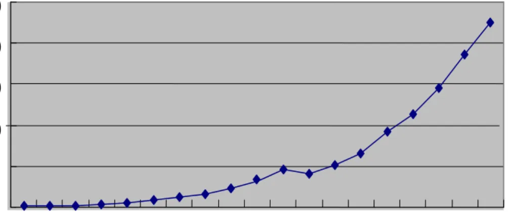
Figure 2.1.1 telecommunications traffic growth trends in 1990—2008 (unit: billion)

0

500 1000

1500

2000

2500

1990 1992 1994 1996 1998 2000 2002 2004 2006 2008

t

Y

(6)

Röda Vägen 3S-781-88 Fax:+46(0)23778080

5

2.1.2 The number of users in Telecommunications

In 2008, telephone subscribers have a net increase of 69.092 million to a total of 982.034 million. The proportion of mobile phone users against the total number of telephone users reaches up to 65.3%, and the number of mobile phone subscribers is 300 million more than fixed telephone subscribers. Fixed telephone subscribers decrease 24.832 million from 340.804 million.

Urban telephone subscribers reduce 16.602 million from 23.1995 million. Telephone users in rural areas reduce 8.23 million from 10.881 million. Fixed-line telephone penetration rate is 25.8/hundred, compared with the previous end of the year, it decreases 2.0/hundred. Traditional fixed-line telephone customers reduce 9.201 million from 27.1873 million. The urban wireless telephone subscribers decrease 15.631 million from 68.931 million. The proportion of urban wireless telephone subscribers in the fixed phone users is reduced from 23.1% to 20.2%.

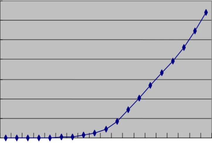
Figure 2.1.2 The number of fixed telephone users, from 1990 to 2008 (unit: 10,000)

0 5000 10000 15000 20000 25000 30000 35000 40000 1990 1992 199419961998 20002002 2004 2006 2008 X8

t

(7)

Röda Vägen 3S-781-88 Fax:+46(0)23778080

6

Figure 2.1.3 Number of mobile phone users trends in 1990—2008 (unit:10,000)

The mobile phone users have a net increase of 93.924 million to 641.23 million. The year of 2008 had the highest growth of mobile phone users where the net increase of mobile phone users have increased 9.458 million in February. The record of a single month increasing has been refreshed. Mobile phone penetration reaches to 48.5/hundred, compared with the previous end of the year, it increases 6.9/hundred. Mobile packet data users increase 94.78 million to 253.925 million. The penetration rate of mobile packet data service increases from 29.1% to 39.6%.

The trend of increasing of the number of fixed phone users from 1990 to 2008 is shown in Figure 2.1.2, and the trend of increasing the number of mobile phone users from 1990 to 2008 is shown in Figure 2.1.3.

2.1.3 Investment in fixed assets

Telecommunications investment in fixed assets achieves 295.37 billion Yuan in 2008. It has grown 29.6%. The net increase of the length of fiber-optic cables in China is 0.991 million kilometers in 2008. In total, it has 6.768 million kilometers instead. The length of distance fiber-optic cables reaches to 793,000 kilometers. Capacity of fixed long-distance telephone exchanges decreases 47,000 Road-sides, but it still has 17.046 million Road-sides. Capacity of office telephone exchanges reduces 1.557 million to 508.789 million. Capacity of mobile telephone exchanges develops 288.546 million to a total of 1.1435 billion. Basic telecommunications enterprise internet broadband access ports grow

0 10000 20000 30000 40000 50000 60000 70000 1990 1992 1994 1996 1998 2000 2002 2004 2006 2008 X7

(8)

Röda Vägen 3S-781-88 Fax:+46(0)23778080

7

23.88 million from 109.28 million. Internet bandwidth of international export reaches to 640286Mbps by increasing 73.6%.

3 Methodology

The essay is an exercise of modeling by multiple linear regression. It studies the quantitative relationship between dependent variable (Aggregate telecommunications) and the independent variables (GDP, The level of household consumption, Total retail sales of social commodities consumption, Renovation investment. The local telephone exchange capacity, Mobile telephone exchange capacity, The amount of the end of mobile phone users, Local telephone end users) by statistical models.

3.1 Multiple linear regression model

Assume that output variable Y is linear regression of input variables X1, X2, X3……X8, with unknown coefficients in the linear regression. The result of the n-observations of input and output will lead to the estimators of the value of coefficients. Usually, we carry out the estimators of all coefficients by least square method.

Multiple linear regression models indicate that:

where y is the dependent variable values, x are independent variables, β are the parameters, and  is the random error term holding the variability that cannot be explained by linear function of x.

3.2 Estimated model

After estimating the parameters in equation (3.1) by the data, we can obtain the estimated model as follows:

To test the existence of significant relation between the dependent variable and all independent variables is called overall test of significance. The method of the test is the comparison between Sum of Squares deviation of Regression (SSR) and Sum of Squares deviations of Residual (SSE). At the same time we also use F tests to analyze whether the difference between SSR and SSE is significant. If there exist significant differences, there will suggest a linear relationship between the dependent variable and the independent

(3.2) (3.1)

(9)

Röda Vägen 3S-781-88 Fax:+46(0)23778080

8

variables. Otherwise, we may consider other models to analyze the data.

3.3 Heteroscedasticity

The definition of Heteroscedasticity is that the explanatory variables for different observations and random error terms have different variance. The idea of heteroscedasticity test is to test correlation between variance of random error term and observed values of explanatory variables. If they have correlation, it is considered to contian heteroscedasticity in the model. To estimate the variance of random error term, the general approximate approach is to use the variance of estimated residuals instead.

3.4 Multicollinearity

If two or more variables have correlation in the regression model, the variables contain multicollinearity. If there appears multicollinearity in the regression, it may lead to the chaos of the estimated models. It can make the analysis to a totally wrong direction. It also can have an impact on the value of parameter estimators, particularly, it may mislead a positive estimator to a negative one.

3.5 AIC and BIC

AIC is the abbreviation of Akaike information criterion. It is a standard measure for the goodness of fitting a statistical model. It was proposed and developed by a Japanese statistician. It can weigh the complexity and the goodness of how the estimated model fit the data. The principle of using the AIC to select variables is: the best model is the model whose AIC value is minimal.

BIC is the abbreviation of Bayesian Information Criterion. The principle of using the BIC to select variables is: the best model is the one whose value of BIC is minimal.

Comparing the method of AIC and BIC, AIC is more conservative. Usually, the number of variables in models which is selected by AIC is larger than the number of variables in the real model. This situation is called over-fitting. However, the number of variables in models which selected by BIC are closer to the real model.

(10)

Röda Vägen 3S-781-88 Fax:+46(0)23778080

9

4 Results

4.1 Analysis by the Full Model

We will use the method of linear regression to establish the model. And to use it we can find the relationship between dependent variable (Aggregate telecommunications) and the independent variables (GDP, The level of household consumption, Total retail sales of social commodities consumption, Renovation investment, The local telephone exchange capacity, Mobile telephone exchange capacity, The amount of the end of mobile phone users, local telephone end users). First of all, we will estimate the full model which contains all independent variables, the results of the estimation are shown in Table 4.1.

From the fitting results, we can get the following conclusions. When GDP grows 1 unit, the aggregate telecommunications will increase 0.24832 units. Other parameters also can be used for a similar understanding. We can draw that GDP, The level of household consumption, renovation investment, the local telephone exchange capacity, Mobile telephone exchange capacity, Local telephone subscribers are positive correlation with the dependent variable. But Total retail sales of social commodities consumption and Mobile phone users are negatively correlated with the dependent variable. This result is clearly not consistent with the actual. Even more, the regression coefficients of the fitted values which are the dependent variable with the most of the independent variables are smaller than normal, and the parameters of significance test of the P-values are too large. Apart from Total retail sales of social commodities consumption, the local telephone exchange capacity and Local telephone subscribers, the parameter estimation of the rest of the independent variables did not pass significance test. However goodness fit of the equation of overall even reached 0.89. This result is obviously unreasonable. We can see from the above conclusion that the linear regression model of the telecommunications revenue is not satisfactory, we have to improve it.

Table 4.1 Full Mode

Variables Coefficient estimate Standard deviation P-value Intercept -10.37171 68.384736 0.28247 GDP 0.24832 0.14904 0.14315

(11)

Röda Vägen 3S-781-88 Fax:+46(0)23778080

10

The level of household consumption

-8.07761 5.52997 0.17479

Total retail sales of social commodities consumption

0.45982 0.21917 0.06228

Renovation investment 0.16020 0.34033 0.64793

The local telephone exchange capacity

0.38191 0.14397 0.02420

Mobile telephone exchange capacity

0.08241 0.05581 0.17053

Mobile phone users -0.24592 0.20137 0.25000

Local telephone subscribers

0.51507 0.15869 0.00878

Notes:

o Standard deviation of residual items 35.04 o Model test of significance P-value 0.0001 o R-Squared 0.8985

o Adjusted R-squared 0.8972

4.2 Model optimization

The next analysis will necessarily focus on the full model for model-based diagnosis. We will test whether various assumptions for the model can be set up, such as heteroscedasticity, normality of Residuals and multicollinearity of the independent variables. And we will also optimize of the equations. Finally we can get a reasonable fitting regression.

4.2.1 Heteroscedasticity Test

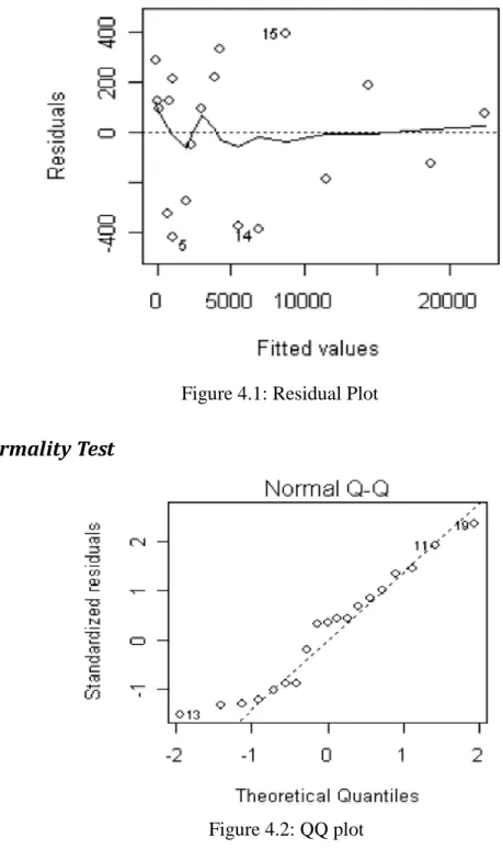
Shown in Figure 4.1, the horizontal axis is the fitted values of the various observations. The vertical axis is the isolated residual. From the figure, the distribution of residuals are disorderly, and it is no clear trend. It shows that the basic assumption of Heteroscedasticity is established.

(12)

Röda Vägen 3S-781-88 Fax:+46(0)23778080

11

Figure 4.1: Residual Plot

4.2.2 Normality Test

Figure 4.2: QQ plot

We use QQ diagram to examine the normality of the residuals. The role of QQ diagram is to sort out the sample residuals. The horizontal axis represents the quantiles of estimated residuals, while the vertical axes represent the theoretical quantiles, drawing their scatters accordingly. If the result of scatter is approximate to straight line, it can be considered to meet the normality assumption. If the result of scatter is relatively large deviation from a straight line, then it does not meet the normality assumption.

(13)

Röda Vägen 3S-781-88 Fax:+46(0)23778080

12

which suggests the normality assumption.

4.2.3 Multicollinearity test

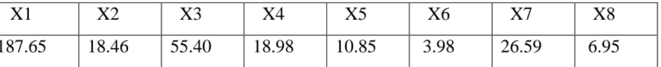
From the equation fitting analysis the results can be clearly found that the majority of the independent variable regression coefficient of the fitted values are small, the parameters of significance test of the P values are generally too large, in addition to retail sales of social commodities the total spending of the local telephone Council exchange capacity and local telephone subscribers of these three indicators, the other five indicators parameter estimate significance test were not passed, However, the overall goodness of fit equation even reached 0.89, this result clearly illustrates the equation variables a multi-co linearity. The reason we care about this issue, because if one or more independent variables to other variables that can be a good linear, then the amount of the reliability of our estimates will be poor. Statistics on the extent of multicollinearity by variance inflation factor (VIF) to measure. VIF reflects the extent to which the first i variables contain information has been covered by other independent variables. Therefore, if an independent variable corresponds to the large VIF value, then blindly adding this variable in the model role will seriously decrease the efficiency of the model. This is because the model would be difficult to distinguish between the independent variables with the other variables of the effect, so the corresponding estimated regression coefficient is very accurate. Through the program output, we carried out detailed analysis of the VIF values of each variable as shown below,

Table 4.2: VIF values of all independent variables

X1 X2 X3 X4 X5 X6 X7 X8

187.65 18.46 55.40 18.98 10.85 3.98 26.59 6.95

As the table shown, most of the parameters of the VIF values are too large; particularly for the first four parameters, the VIF values are greater than 10. Therefore, we should consider multicollinearity in the model. In fact, such a phenomenon also can be explained, because independent variables included in the model are closely related to social development, especially the first four independent variables, the household consumption levels, retail sales of social commodities, investment in upgrading and updating of the total spending is likely as domestic GDP growth, growth, consumption levels, retail sales of social commodities, investment in upgrading and updating of the total spending of these

(14)

Röda Vägen 3S-781-88 Fax:+46(0)23778080

13

three variables are likely to be linear Biaochu gross domestic product. Therefore, the response to the original equation in the variable variant of the individual in order to eliminate or improve during the multi-co linearity makes the model more convincing.

The study of differential equations method to the self-variables variant of the use of gross national product, will the consumer level, retail sales of social commodities, investment in upgrading and updating of the total spending of these four variables, the amount of annual growth as a new variable substituted into Equation new parameters in order to eliminate multiple variables co linearity.

After a variable of modified equations, through the R program analysis, obtained the following results:

Table 4.3: Variant independent variables after the VIF value of statistical tables

ΔX1 ΔX2 ΔX3 ΔX4 X5 X6 X7 X8

7.39 12.69 9.41 10.03 9.92 3.76 24.56 7.31

From the above table may, but that all parameters of the VIF values are also reduced, most of the parameters of the VIF values are below 10 shows the basic model variant has improved after the independent variable multicollinearity. Although not all of the parameters are inflated by a variance factor test, but the model of choice, taking into account the special nature of the variables, since the multicollinearity between the variables is basically impossible to fundamentally eliminate. Therefore, this analysis will ignore the resulting error, that the adoption of this model, the basic test of multicollinearity. As a result, we can consider this model to some extent to meet the linear model of all the important assumptions. At this point right after the model variant is estimated that the estimation results obtained are as follows.

The model parameters have largely adopted a significance test, the overall sentence coefficient decreased, in order to 0.8385, indicating the overall model fit is also very effective.

(15)

Röda Vägen 3S-781-88 Fax:+46(0)23778080

14

Table 4.4: Full model after the variant

Variables Coefficient estimate Standard deviation P-value Intercept -14.3717 0.3321 0.0625 GDP 8. 7761 0.0671 0.0044

2.2487 0.0443 0.0328

Total retail sales of social commodities consumption

0.5982 0.1752 0.2744

0.8191 0.1939 0.1562

1.2413 0.0236 0.0026

Mobile phone users 0.02459 0.5831 0.3727

Local telephone subscribers 0.0507 0.6307 0.2862

Notes:

o Standard deviation of residual items 0.7379 o Model test of significance P-value 0.0001 o R-Square 0.8385

4.3 Model Selection

From the analysis above, it is easy to find that there are three important variables, gross domestic product, the level of annual consumption, and mobile switching capacity of the dependent variable, but we cannot rule out other variables which have the interpretation of the telecommunications traffic capacity. Therefore, we commonly used two kinds of method of selection of variables, AIC and BIC, to select the better model.

If you use the AIC to select the model, we can get the following model to estimate the results, as shown in Table 4.5.

(16)

Röda Vägen 3S-781-88 Fax:+46(0)23778080

15

Table 4.5: AIC results

9.4125 3.1987 0.0123

0.5717 0.0408 0.0871

0.1905 0.0282 2.06e-05

Notes:

The first six variables (mobile switching capacity) are very important to explain the Prime Minister of telecommunication services. Moreover, all the variables selected in the level of 0.10 under the world significantly, and its judgments coefficient decreased relative to the full model shows that self-colinearity between the variables have also been

eliminated, 0.7291 goodness of fit is also acceptable. If you use BIC to select models, you can see the following model to estimate the results, as shown in Table 4.6.

Can be seen from the table, AIC that the first one variable (GDP), the first two variables (the consumer level) and six variables (mobile switching capacity) to explain the Prime Minister of telecommunication services is very important. But it does not think the first four variables (renovation investment), the first five variables (the local telephone exchange capacity) is also very important. And BIC selected all the variables are the level of 0.05 is significant.

(17)

Röda Vägen 3S-781-88 Fax:+46(0)23778080

16

understand what indicators to explain the volume of telecommunications services provide a theoretical basis. Further analysis, from a good explanatory power, simplicity, and relatively conservative point of view, AIC selected model is able to provide more theoretical thinking.

Table 4.6: BIC results

5.7318 0.08989 0.0174

11.2390 0.01434 1.25e-10

Notes:

(18)

Röda Vägen 3S-781-88 Fax:+46(0)23778080

17

5 Conclusion

Through the above analysis, we finally decide to use the AIC model. From the model results, we can find out that the GDP, Consumption Levels, Renovation Investment, the Local Telephone Exchange Capacity and Mobile Switching Capacity are the main factors to the Total Telecom Business. According to their respective regression coefficient, we can sort the order of the dependent variables which is the Mobile Switching Capacity, GDP, Consumption Levels, Investment in Building Renovation, the Local Telephone Office Exchange Capacity. This result is consistent with China's national conditions. As the economy continues to develop, the mobile communication play an increasingly important role in people's leisure life and it has become an indispensable part of life that there is much momentum to replace the fixed-line communications.

The first year of creating mobile phone business in 1987, there are only 700 households nationwide customers. The first five years, i.e. 1987-1991 the users of mobile phone develop to 48000; the second five-year develop to 6.805 million users, the number of users is 142 times for the first five years. While from 1997 to 1999, the number of mobile phone users had reached 24.237 million, is the 505 times of the first five-year users. In 20 years, the number of mobile phone users had grown with 171 percent average annual, and the growth rate of the rapid development has made achievements that have attracted worldwide attention. As the end of 2008, China's mobile phone users reached 640 million. the amount is the highest in the world. Therefore, the number of mobile phone users is no doubt the fastest growth factor in total business volume of China's telecommunications, and the development has made important contributions for the growth of economic.

Second, the factors which impact of telecommunications revenue are GDP and Consumption Level. And these two variables can also impact on part of China’s economic benefits. Telecommunications revenue development and economic growth are mutually reinforcing, and this influence can not be ignored. When the personal revenue has risen, people in telecommunication spending will certainly increase.

Compared to other factors, the local telephone exchange capacity impact on the telecommunications revenue is minimal. But the fixed-line telephone communications is a fundamental business of the telecommunications industry, its contribution to total telecommunications services has been replaced by increasingly mobile communications in

(19)

Röda Vägen 3S-781-88 Fax:+46(0)23778080

18

recent years. According to data analysis, we find that as the mobile communications had gradually increase the contribution in the telecommunications industry, the fixed communication is likely to be replaced by mobile communication service in the future. This is an inevitable social development.

(20)

Röda Vägen 3S-781-88 Fax:+46(0)23778080

19

Appendix

Variables Definition Description

Y Aggregate

telecommunications

It refers to the magnitude of value forms of telecommunications companies provide the community

with the total number of various types of

telecommunications services. It reflects the

comprehensive development of the overall

telecommunications business results in a certain period; it is also the key indicators to study the composition and development of telecom business volume trends

X1 Gross Domestic

Product

The total market value of all final goods and services produced in a country in a given year, equal to total consumer, investment and government spending, plus the value of exports, minus the value of imports

X2 The level of

household consumption

It refers to resident households on goods and services of all final consumption expenditure. The price of household is calculated at market price

X3 Total retail sales of social commodities consumption

It refers to the national economy directly sold the total amount of consumer goods to urban and rural residents in various sectors and social groups. It is a reflection of the industry through a variety of commodity circulation channels to provide the total supplication of consumer goods to the residents and social groups. It is an important indicator to study the changes in the domestic retail market and the reflecting of the degree of economic boom

X4 Renovation

investment

It refers to the technological transformation of fixed assets and existing facilities in social groups. Its comprehensive range is renovation project of the total invested over 50 million Yuan.

X5 The local telephone exchange capacity

Means for the continuation of the exchange capacity of local telephone

(21)

Röda Vägen 3S-781-88 Fax:+46(0)23778080

20

X6 Mobile telephone

exchange capacity

Means for the continuation of the exchange capacity of mobile phones.

X7

The amount of the end of mobile phone users)

It refers to the users who register in the mobile phone business divisions, access to Mobile Telephone Network by using Mobile Phone Switch and possession of mobile phone number. The actual number of users is calculated by the amount of the user who has been registered into the postal service mobile telephone network; one mobile phone is defined as a unit.

X8 Local telephone end users

It refers to phone users who had already accessed to national public fixed telephone network and have been managed by the fixed telephone services.

(22)

Röda Vägen 3S-781-88 Fax:+46(0)23778080

21

References

[1] Gao, Y. 2003. The statistical analyze of the market segmentation of telecom major clients. Journal of Zhengzhou Institute of Aeronautical Industry Management, 6, 76-79.

[2] Ju, L. 1996. The communication scale of the annual investment in the economic analysis. VIP Information, 4, 32-36.

[3] Liao, J. 2006. China Mobile Communication Industry Model Analysis. China New Telecommunications, 9, 5-11.

[4] Liu, J., Liu, Q., Xiang, O. 2007. Beijing telecommunications industry and the global comparative analysis of the basic profile. Communication World, 27-29.

[5] Ma, S. 2003. Analysis of the telecommunications market segmentation strategy. CATR, 19-23.

[6] Sun, J. 2007. Interpretation of China's telecommunications industry context. Communication World, 3,14.

[7] Wang, J., Zhou, W., Liu, Y. 2004. Economic Analysis of quality of telecommunications services. Journal of China University of Posts and Telecommunications, 7, 23-26.

[8] Wang, Q. 2005. Telecom Industry Customer Satisfaction Study. Telecommunications Technology, 1, 17-22.

[9] Xiong, J. 2006. Zhejiang information industry development and economic growth effects of the statistical analysis of Telecommunications Technology. Economics, 10-12.

[10] Yao, L. 2003. On the telecom enterprise value and customer resource management model. Marketing Week, 4, 21-24.

[11] Yi, C., Wan, J. Statistical analysis of China's telecommunications revenue. Statistics and Decision, 9, 114-115

[12] 2007. Analysis on operation of the communications industry in 2007. Communication Enterprise Management, 12, 77-78.

[13] 2007. Development Trend of China's telecom industry. Network Telecommunications Information Research Center, 2, 33-35.

An Analysis of the Telecommunications Business in China by Linear Regression