Analysis of Speed Sign Classification Algorithms Using Shape Based Segmentation of Binary Images

X. Jiang and N. Petkov (Eds.): CAIP 2009, LNCS 5702, pp. 1220–1227, 2009. © Springer-Verlag Berlin Heidelberg 2009

Shape Based Segmentation of Binary Images

Blekinge Institute of Technology, SE-372 25 Ronneby, Sweden {azam.sheikh.muhammad,niklas.lavesson,paul.davidsson,

mikael.nilsson}@bth.se

Abstract. Traffic Sign Recognition is a widely studied problem and its dynamic

nature calls for the application of a broad range of preprocessing, segmentation, and recognition techniques but few databases are available for evaluation. We have produced a database consisting of 1,300 images captured by a video cam-era. On this database we have conducted a systematic experimental study. We used four different preprocessing techniques and designed a generic speed sign segmentation algorithm. Then we selected a range of contemporary speed sign classification algorithms using shape based segmented binary images for train-ing and evaluated their results ustrain-ing four metrics, includtrain-ing accuracy and processing speed. The results indicate that Naive Bayes and Random Forest seem particularly well suited for this recognition task. Moreover, we show that two specific preprocessing techniques appear to provide a better basis for con-cept learning than the others.

Keywords: Traffic Sign Recognition, Segmentation, Classification.

1 Introduction

Automatic Traffic Sign Recognition (TSR) systems attempt to detect and recognize traffic signs from live images captured by a video camera mounted on a vehicle. The development of such a visual pattern recognition system is not a trivial task [1]. It has attracted the research community since the eighties [2]. There are a number of issues associated with the automatic detection and classification of traffic sign patterns from real-world video or images. Visibility is the key issue in the performance of a TSR system because it determines the quality of the captured images and hence affects classification performance. A TSR system can only attract the transport community if it can outperform, or at least perform comparably to, humans in correctly locating and recognizing signs at low visibility. Visibility issues can arise due to many reasons. For instance, the various lighting conditions at different hours of the day and the different seasons have a strong impact on visibility. Additionally, because of trees or shadows of nearby buildings the signs may be partially hidden. These and other common issues have been discussed in related studies [1]. Researchers have applied a variety of pre-processing techniques based on color pre-processing [3, 4], shape analysis [3-5], along with numerous classification and recognition techniques ranging from template matching algorithms [3, 6], Radial Basis Function (RBF) Network [7, 8], Multilayer

Perceptron and other Neural Networks [7, 8], Genetic Algorithms [9], Fuzzy Logic [10] to the applications of Support Vector Machines [11] and signal processing-based transformation-specific classifiers.

Accuracy and processing speed are two important performance metrics in the de-velopment of TSR systems. Some studies present detection and/or classification re-sults around 90% [12, 13] or in some cases 95% [10] or more. However, few studies compare with other databases than their own and the used database is seldom made public. Moreover, the level of detail in describing the preprocessing and other steps is usually low, which makes it difficult to reproduce the experiment. Besides related work and also some commercial implementations of TSR systems [14] there are prac-tically no significant traffic sign databases available. We have only managed to find a small database, consisting of 48 images of three different traffic signs, available on-line [15]. This study aims to remedy this situation by making our initial database publicly available. We also expect to enlarge the database in future work. For the initial database, we have collected 1,300 images from Swedish roads. Detection and recognition of speed signs in particular have been extensively studied [13, 16, 17]. In this work our main focus is to conduct an extensive study on various algorithms for the classification of this particular type of sign. For this purpose we extract the shape based binary information from the sign images to generate training and testing data sets for supervised concept learning. A number of classifiers are evaluated for speed limit recognition under various performance metrics. In order to make the preprocess-ing, segmentation and classification experiments reproducible, standard tools are used and each step is described in detail. Our database of traffic sign images and the im-plementation results are available online1.

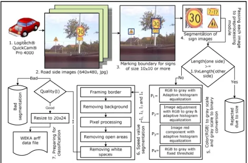
Fig. 1. Traffic signs collection & processing

1

2 Data Collection, Size Analysis and Preprocessing

We collected 1,300 raw images of the traffic signs using a Logitech Quick Cam Pro 4,000 web camera with automatic settings and a resolution of 640×480 for each im-age. The collection of images along road sides was performed during different hours of the day, and thus under various lighting conditions to maximize visibility disorders. Since this study is concerned with speed signs only, each such sign (30, 50, 70, 90 and 110) is marked and associated with a corresponding class. We also considered multiple speed signs present in a single image and included a reasonable collection of non-speed signs as well. We labeled such signs as belonging to the Noise class. In Fig. 1, steps 1 to 4 describe the image capturing, boundary marking and the segmenta-tion of sign images from the original image for further processing. During boundary marking (step 3 in Fig. 1) we have marked signs of size 10×10 pixels or more.

A traffic sign detection algorithm has to process images that include rectangular shapes, as opposed to the circular shape of the speed signs. Thus, we also marked rectangular signs as well as some non-sign rectangular shapes. To avoid unnecessary processing of rectangular shapes and to make the system robust against non-speed signs, a basic size analysis is conducted before passing the sign image to the prepro-cessing module. We have analyzed the height and width of the images for each class in our database, and can conclude that, for all of the properly segmented speed signs as well as other traffic sign images, the height and width are almost identical. For the other images the height is roughly 1.5 times the width. So, in our size analysis heuris-tic approach, we simply discard an image if the width of the image is 1.9 times the height or vice versa. We have kept this threshold slightly flexible just to ensure that no speed sign image is rejected. This check is shown after step 4 in Fig. 1.

There are several methods based on shape or color information that can be used ei-ther individually, or in combination, for this purpose. The reader may refer to [1] for a detailed study on such techniques. We have chosen to process signs based on shape because similarity matching between templates is considered good for classification algorithms [1]. For this purpose we need to convert color images to binary images. Binary images are very economical as opposed to color images with respect to the training and testing times required for the classification algorithms. Thus the scope of our preprocessing module is to take the color image and to convert it to a gray scale image, which is then further processed to get a binary (black and white) image. To ensure an unbiased evaluation of the classifiers, we implemented four different tech-niques in the preprocessing module. For our preprocessing, critical decisions need to be made with regard to 1) the selection of technique for color to grayscale conversion and 2) which gray threshold to use in order to generate the binary image.

We therefore made different choices for these decisions and developed four inva-riants, as shown with labels P1, P2, P3 and P4 respectively in step 5 of Fig. 1. Our

im-plementation of P1 through P4 includes regular MATLAB functions for color image to

gray scale conversion, adaptive histogram equalization and gray level threshold for conversion to binary. For the implementation of P1 rgb2gray is used to convert from

color image to gray image then adapthisteq, graythresh, and im2bw are applied in sequence to get the binary image. In P2 the input image is first adjusted with regard to

color intensities. For this purpose the function imadjust is used and the input parame-ter [low_in; high_in] is given as [0.3 0.2 0.1; 0.8 0.6 0.8]. We have analyzed the

results using various sets of values for this parameter and heuristically we have con-cluded that the above given set of values produces sufficiently good results. The adjusted image is then processed similar to P1. For P3 we used the intensity of the red

component from the color image as the gray level to get a gray image. The remaining steps are the same as for P1. In P4, the same method as the one used for P1 is followed,

but the gray threshold is further processed so that, if the threshold θ is greater than ½, it is recalculated as defined below:

,

, (1)

We have developed a technique consisting of six simple steps of sequential processing for possible segmentation of the speed limit value as shown in step 6 of Fig. 1. Our segmentation logic is independent of the preprocessing techniques dis-cussed above. Output binary images I1, I2, I3 and I4 from the preprocessing P1 through

P4 form the input to the segmentation module. The same segmentation steps are

ap-plied on each of I1 through I4, separately. The first step is the framing border, which

ensures maximum reduction of the background noise. Black borders are added in the background with a size of 10% of the length of each side. Then, in the next step the background noise is filtered by removing 4-connected neighborhood pixels. It also removes the frame generated during the previous step. In the third step, the isolated black pixels and single pixel connected black lines are converted to white. This process removes small clusters of noise and separates single pixel connected black regions. After step three, some large clusters of noise in the form of groups of con-nected black pixels still exist. We call them open areas since they are not part of the shape of the speed limit value. We remove them in the fourth step. This time we search for 8-connected neighbors and remove those open areas which have a pixel count below a certain threshold. The threshold pixel count (Pc) is taken as the percen-tage of black pixels in the image plus some constant integer value such as 7 or 8. This step also ensures that the speed limit value is not affected. Next, we remove white spaces from all four sides and define a bounding box for the segmented speed limit value. After step five, the segmentation process is over. The last step is basically to determine the quality of the segmented image. We define segmentation quality as either good or bad. If the quality is good, the image is resized to a predefined width and height, so that each instance given to the classifier is of the same size. The dimen-sion of the resized images is 20×24, a dimendimen-sion which was determined by taking the average size of the segmented images based on the output of the four preprocessing methods. The quality analysis is the most important (and the most technical) step in the segmentation algorithm. We will now discuss why quality analysis is important and describe our quality analysis approach.

Normally, on the road sides there are a lot of different signs and speed signs appear rarely. For example, in our collection only 20% of the images represent speed signs. Since we are only concerned with the speed sign images, we classify each non-speed sign as Noise. For this purpose, a proper shape segmentation of the speed limit value is desired. At the same time, it is important to design robust criteria to deal with non-speed signs. It is not a good idea to simply use every non-non-speed sign image as a mem-ber of the Noise class. Non-speed signs do not follow any predefined pattern and thus

it will be difficult for a classifier to properly learn the Noise class. During segmenta-tion, any prior information about the class of the input image is not present and it is upon the segmentation method to reject as many of the noisy images as possible. Thus, during the last step of the segmentation process we analyze the images based on the quality criteria shown in Eqn. 2. A binary decision in terms of good or bad quality is made for each segmented image. Bad segmentations are discarded whereas good segmentations are normalized with regard to size and used for the further preparations for classification. , , 13, 13, 3 1, , , (2)

Our quality analysis is independent of the preprocessing and segmentation tech-niques. The quality check serves two main purposes. It allows the selection of all well segmented speed sign images by marking them as good quality and rejecting poor segmentation results by labeling them as bad quality segmentation to achieve a high hit ratio. Secondly, when we apply the check on the segmentation results of noisy images, most of them are simply rejected as being bad segmentations. Thus, the non-speed signs that are regarded as good quality after the segmentation process are the only non-speed signs that will be included in the Noise class. Therefore a classifica-tion as good is expected for each speed sign while bad is desired for every non-speed sign. The segmentation quality analysis is also robust against visibility disorders of the images and tries to reject most of them to avoid misclassifications at the later stage. The experimental results seem to indicate that all four preprocessing techniques perform well in rejecting non-speed signs, since 95% to 98% of these signs are put into the bad segmentation collection.

3 Analysis of Classification Algorithms

From the segmentation results we get the shape representation of the sign as binary images. To conduct the experiments we use the Weka [18] machine learning workbench. To examine the classification results separately for each preprocessing technique, we constructed four ARFF-based data sets. These data sets include six different classes: the speed limit values 30, 50, 70, 90, 110, and the Noise class. Segmentation results for each preprocessing technique are associated with the re-spective class labels and thus a training data set of binary strings for each prepro-cessing is generated. To convert the training set into Weka ARFF format we defined a relation consisting of 480 nominal attributes, each corresponding to the binary value of a pixel.

3.1 Algorithm Selection and Performance Analysis

The main objective of our experiments is to evaluate the performance of different classification algorithms for the speed sign recognition problem. The generated clas-sifiers are evaluated based on the results from all four data sets. We have selected a diverse population of 15 algorithms from different learning categories (e.g., Percep-tron and Kernel functions, Bayesian learners, Decision trees, Meta-learners, and Rule inducers), see Table 1 column one. We used Weka algorithm implementations and tried various parameter configurations but observed no significant difference in clas-sifier performance as compared to the default configuration, except for Multilayer Perceptron. We observed that, with 8 neurons in the hidden layer and the learning rate set to 0.2 (the default is 0.3) the same recognition performance was achieved, but a significant decrease in training time was achieved.

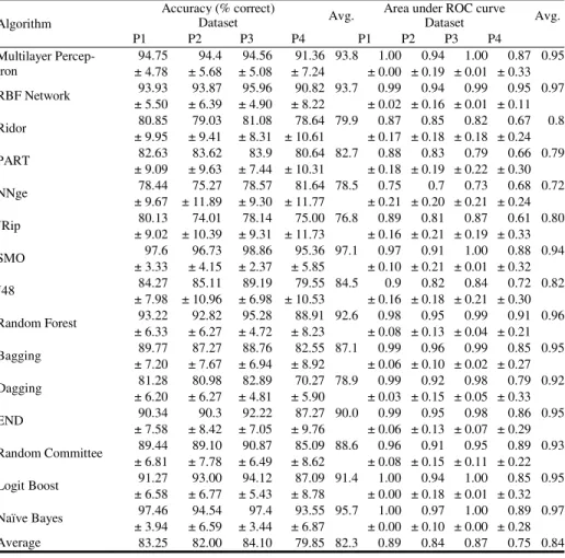
Table 1. Experiment results for accuracy and AUC

Algorithm

Accuracy (% correct)

Avg. Area under ROC curve Avg.

Dataset Dataset P1 P2 P3 P4 P1 P2 P3 P4 Multilayer Percep-tron 94.75 94.4 94.56 91.36 93.8 1.00 0.94 1.00 0.87 0.95 ± 4.78 ± 5.68 ± 5.08 ± 7.24 ± 0.00 ± 0.19 ± 0.01 ± 0.33 RBF Network 93.93 93.87 95.96 90.82 93.7 0.99 0.94 0.99 0.95 0.97 ± 5.50 ± 6.39 ± 4.90 ± 8.22 ± 0.02 ± 0.16 ± 0.01 ± 0.11 Ridor 80.85 79.03 81.08 78.64 79.9 0.87 0.85 0.82 0.67 0.8 ± 9.95 ± 9.41 ± 8.31 ± 10.61 ± 0.17 ± 0.18 ± 0.18 ± 0.24 PART 82.63 83.62 83.9 80.64 82.7 0.88 0.83 0.79 0.66 0.79 ± 9.09 ± 9.63 ± 7.44 ± 10.31 ± 0.18 ± 0.19 ± 0.22 ± 0.30 NNge 78.44 75.27 78.57 81.64 78.5 0.75 0.7 0.73 0.68 0.72 ± 9.67 ± 11.89 ± 9.30 ± 11.77 ± 0.21 ± 0.20 ± 0.21 ± 0.24 JRip 80.13 74.01 78.14 75.00 76.8 0.89 0.81 0.87 0.61 0.80 ± 9.02 ± 10.39 ± 9.31 ± 11.73 ± 0.16 ± 0.21 ± 0.19 ± 0.33 SMO 97.6 96.73 98.86 95.36 97.1 0.97 0.91 1.00 0.88 0.94 ± 3.33 ± 4.15 ± 2.37 ± 5.85 ± 0.10 ± 0.21 ± 0.01 ± 0.32 J48 84.27 85.11 89.19 79.55 84.5 0.9 0.82 0.84 0.72 0.82 ± 7.98 ± 10.96 ± 6.98 ± 10.53 ± 0.16 ± 0.18 ± 0.21 ± 0.30 Random Forest 93.22 92.82 95.28 88.91 92.6 0.98 0.95 0.99 0.91 0.96 ± 6.33 ± 6.27 ± 4.72 ± 8.23 ± 0.08 ± 0.13 ± 0.04 ± 0.21 Bagging 89.77 87.27 88.76 82.55 87.1 0.99 0.96 0.99 0.85 0.95 ± 7.20 ± 7.67 ± 6.94 ± 8.92 ± 0.06 ± 0.10 ± 0.02 ± 0.27 Dagging 81.28 80.98 82.89 70.27 78.9 0.99 0.92 0.98 0.79 0.92 ± 6.20 ± 6.27 ± 4.81 ± 5.90 ± 0.03 ± 0.15 ± 0.05 ± 0.33 END 90.34 90.3 92.22 87.27 90.0 0.99 0.95 0.98 0.86 0.95 ± 7.58 ± 8.42 ± 7.05 ± 9.76 ± 0.06 ± 0.13 ± 0.07 ± 0.29 Random Committee 89.44 89.10 90.87 85.09 88.6 0.96 0.91 0.95 0.89 0.93 ± 6.81 ± 7.78 ± 6.49 ± 8.62 ± 0.08 ± 0.15 ± 0.11 ± 0.22 Logit Boost 91.27 93.00 94.12 87.09 91.4 1.00 0.94 1.00 0.85 0.95 ± 6.58 ± 6.77 ± 5.43 ± 8.78 ± 0.00 ± 0.18 ± 0.01 ± 0.32 Naïve Bayes 97.46 94.54 97.4 93.55 95.7 1.00 0.97 1.00 0.89 0.97 ± 3.94 ± 6.59 ± 3.44 ± 6.87 ± 0.00 ± 0.10 ± 0.00 ± 0.28 Average 83.25 82.00 84.10 79.85 82.3 0.89 0.84 0.87 0.75 0.84

Multilayer Perceptron is the most widely used [7, 9] algorithm in TSR applications, especially for speed sign recognition. Consequently, we used it as the base classifier in Weka (with optimized parameters) and all other classifiers (generated with default configurations) are evaluated against it. In addition to Multilayer Perceptron, RBF Network and Support Vector Machines are also used in a number of related studies, as described earlier. Thus, it was natural to include these algorithms in our experiments. We performed ten 10-fold cross-validation tests and used the corrected paired t-test (confidence 0.05, two-tailed) for all four data sets. We compared the performance based on four evaluation metrics; accuracy, the Area under the ROC curve (AUC), training time, and testing time. The experimental results are shown in Table 1. The average performance over all data sets is also presented in the Table. With respect to accuracy and AUC, we observe that the best performing algorithms are: Multilayer Perceptron, RBF Network, SMO (Weka implementation of SVM), Random Forest, and Naive Bayes. Now we consider the training and testing time. Besides accuracy, the elapsed time is also very important in the performance evaluation of classifiers, with respect to the application at hand. An analysis of training and testing times de-monstrates that, among our best algorithms with respect to accuracy and AUC, Ran-dom Forest and Naive Bayes are by far the fastest algorithms with regard to both training and testing. From the results we can conclude that, aside from good perfor-mance by the commonly used classifiers for this problem, Naive Bayes and Random Forest have achieved quite promising results in terms of accuracy and significantly better training and testing times than the other algorithms. We have also analyzed the results of the individual preprocessing techniques. For almost all of the 15 algorithms and specially the above mentioned five algorithms, P1 and P3 have shown consistently

a higher accuracy than P2 and P4. We can also observe that both P1 and P3 have better

AUC values than the other two techniques.

4 Conclusion and Future Work

Our proposed size analysis criterion is able to properly differentiate the detected traf-fic signs from those of under or over segmented signs and other noisy segmentations. The criterion is database independent and hence it can be applied to any collection of traffic sign images. Due to the real-time nature of TSR applications, a short recogni-tion time in conjuncrecogni-tion with good accuracy is always desirable. This is indeed an important trade-off for most real-time recognition systems. The experimental results indicate that Naive Bayes and Random Forest are quite accurate and have better train-ing and testtrain-ing times than the other studied algorithms. We conclude that our ap-proach is suitable, at least for the studied database. In addition, we have evaluated four preprocessing techniques. Experiments indicate that P1 and P3 are more suitable

for preprocessing speed signs. Moreover, we have introduced the concept of segmen-tation quality analysis and proposed a general speed limit value segmensegmen-tation tech-nique. The two preprocessing techniques together with the segmentation algorithm provide a good basis for the development of a TSR system using the proposed clas-sifiers. For future work, we intend to collect a larger database incorporating all types of traffic signs.

References

1. Nguwi, Y.Y., Kouzani, A.Z.: A study on automatic recognition of road signs. In: 2006 IEEE Conference on Cybernetics and Intelligent Systems, pp. 1–6 (2006)

2. Mace, D.J., Pollack, L.: Visual Complexity and Sign Brightness in Detection and Recogni-tion of Traffic Signs. TransportaRecogni-tion Research Record HS-036 167(904), 33–41 (1983) 3. Malik, R., Khurshid, J., Ahmad, S.N.: Road Sign Detection and Recognition using Colour

Segmentation, Shape Analysis and Template Matching. In: 6th International Conference on Machine Learning Cybernetics, pp. 3556–3560 (2007)

4. Andrey, V., Hyun, K.: Automatic Detection and Recognition of Traffic Signs using Geometric Structure Analysis. In: SICE-ICASE International Joint Conference, pp. 1451–1456 (2006) 5. Cyganek, B.: Real-time detection of the triangular and rectangular shape road signs. In:

Blanc-Talon, J., Philips, W., Popescu, D., Scheunders, P. (eds.) ACIVS 2007. LNCS, vol. 4678, pp. 744–755. Springer, Heidelberg (2007)

6. Cyganek, B.: Road Signs Recognition by the Scale-space Template Matching in the Log-polar Domain. In: Martí, J., Benedí, J.M., Mendonça, A.M., Serrat, J. (eds.) IbPRIA 2007. LNCS, vol. 4477, pp. 330–337. Springer, Heidelberg (2007)

7. Nguwi, Y.Y., Kouzani, A.Z.: Automatic Road Sign Recognition using Neural Networks. In: IEEE International Joint Conference on Neural Networks, pp. 3955–3962 (2006) 8. Zhang, H., Luo, D.: A new method for traffic signs classification using probabilistic neural

networks. In: Wang, J., Yi, Z., Zurada, J.M., Lu, B.L., Yin, H. (eds.) ISNN 2006. LNCS, vol. 3973, pp. 33–39. Springer, Heidelberg (2006)

9. Aoyagi, Y., Asakura, T.: Detection and Recognition of Traffic Sign in Scene Image using Genetic Algorithms and Neural Networks. In: 35th SICE Annual Conference, pp. 1343–1348 (1996) 10. Fleyeh, H., Gilani, S.O., Dougherty, M.: Road Sign Detection and Recognition using

Fuzzy ARTMAP: a case study Swedish speed-limit signs. In: 10th IASTED International Conference on Artificial Intelligence and Soft Computing, pp. 242–249 (2006)

11. Maldonado-Bascon, S., Lafuente-Arroyo, S., Gil-Jimenez, P., et al.: Road-Sign Detection and Recognition based on Support Vector Machines. IEEE Transactions on Intelligent Transportation Systems 8(2), 264–278 (2007)

12. Soetedjo, Y.K.: Traffic Sign Classification using Ring Partitioned Method. IEICE Trans. on Fundamentals E88(9), 2419–2426 (2005)

13. Torresen, J., Bakke, J.W., Sekanina, L.: Efficient Recognition of Speed Limit Signs. In: 7th International IEEE Conference on Intelligent Transportation Systems, pp. 652–656 (2004) 14. Siemens: Siemens VDO 2007 (2007),

http://usa.vdo.com/products_solutions/cars/adas/ traffic-sign-recognition/

15. Grigorescu, P.N.: Traffic Sign Image Database,

http://www.cs.rug.nl/~imaging/databases/

traffic_sign_database/traffic_sign_database_2.html

16. Cao Tam, P., Elton, D.: Difference of Gaussian for Speed Sign Detection in Low Light Conditions. In: International MultiConference of Engineers and Computer Scientists, pp. 1838–1843 (2007)

17. Moutarde, F., Bargeton, A., Herbin, A., et al.: Robust On-vehicle Real-time Visual Detec-tion of American and European Speed Limit Signs with a Modular Traffic Signs Recogni-tion System. In: IEEE Intelligent Vehicles Symposium, pp. 1122–1126 (2007)

18. Witten, H., Frank, E.: Data Mining: Practical Machine Learning Tools and Techniques, 2nd edn. Morgan Kaufmann, San Francisco (2005)