Analysis and correlation of growth strata of the Cretaceous to Paleocene Lower Dawson Formation: insight into the tectono-stratigraphic evolution of the Colorado Front Range

(1)

ANALYSIS AND CORRELATION OF GROWTH STRATA OF THE CRETACEOUS TO PALEOCENE LOWER DAWSON FORMATION: INSIGHT INTO THE

TECTONO-STRATIGRAPHIC EVOLUTION OF THE COLORADO FRONT RANGE

by

(2)

A thesis submitted to the Faculty and Board of Trustees of the Colorado School of Mines in partial fulfillment of the requirements for the degree of Master of Science (Geology). Golden, Colorado Date __________________________ Signed: ________________________ Korey Harvey Signed: ________________________ Dr. Jennifer Aschoff Thesis Advisor Golden, Colorado Date ___________________________ Signed: _________________________ Dr. Paul Santi Professor and Head Department of Geology and Geological Engineering

(3)

ABSTRACT

Despite numerous studies of Laramide-style (i.e., basement-cored) structures, their 4-dimensional structural evolution and relationship to adjacent sedimentary basins are not well understood. Analysis and correlation of growth strata along the eastern Colorado Front Range (CFR) help decipher the along-strike linkage of thrust structures and their affect on sediment dispersal. Growth strata, and the syntectonic

unconformities within them, record the relative roles of uplift and deposition through time; when mapped along-strike, they provide insight into the location and geometry of structures through time. This paper presents an integrated structural- stratigraphic analysis and correlation of three growth-strata assemblages within the fluvial and fluvial megafan deposits of the lowermost Cretaceous to Paleocene Dawson Formation on the eastern CFR between Colorado Springs,CO and Sedalia, CO. Structural attitudes from 12 stratigraphic profiles at the three locales record dip discordances that highlight syntectonic unconformities within the growth strata packages. Eight traditional-type syntectonic unconformities were correlated along-strike of the eastern CFR distinguish six phases of uplift in the central portion of the CFR. The correlation of the syntectonic unconformities shows diachronous development of emerging structures that formed the CFR. The structures first developed in the South, then propagated in a northward

direction along the eastern side of the CFR. Lithofacies and paleocurrent analysis within the growth strata record the transition from fluvial (confined) deposition to unconfined fluvial/megafan deposition. Sediment entry points for the fluvial (confined) and

unconfined fluvial/megafan depositional systems were controlled by the lateral linking of along strike thrust faults (i.e., transverse or transfer zones) that bound the CFR.

(4)

Provenance analysis supports the linkage of thrust structures controlling the

provenance and sediment entry points to the Denver Basin. Petrographic analysis of twelve thin sections within the lower Dawson Formation shows two distinct petrofacies indicative of two fluvial megafan systems when considered with lithofacies and

paleocurrent analysis. An unroofing signal was also identified that developed in

response to the removal of Phanerozoic cover and Precambrian basement that covered the CFR due to emerging Laramide structures. The study has implication for predicting clastic sediment distribution in punctuated foreland basins, which ultimately controls reservoir presence for conventional plays and clay content for unconventional shale plays.

(5)

TABLE OF CONTENTS ABSTRACT………...iii LIST OF FIGURES………..ix LIST OF TABLES………...………...…..xxvii ACKNOWLEDGEMENTS………...xxix CHAPTER 1 INTRODUCTION………...1 1.1 PURPOSE OF STUDY………...1

1.2 PREVIOUS COLORADO FRONT RANGE MODELS OF LARAMIDE UPLIFT………...………...2

1.2.1 GEOLOGICAL CONTEXT...3

1.2.2 ORIGINS OF THE LARAMIDE OROGENY...4

1.2.3 KINEMATIC MODELS OF THE CFR...6

1.3 LARAMIDE-STYLE STRUCTURES AND GROWTH STRATA...7

1.4 UNROOFING SIGNALS IN THE DENVER BASIN...8

1.5 METHODS AND DATA...9

1.6 ORGANIZATION OF THESIS...11

REFERNCES CITED...23

CHAPTER 2 ADDING THE 4TH DIMENSION: A RECORD OF LATERAL FAULT LINKING ALONG THE COLORADO FRONT RANGE USING GROWTH STRATA ANALYSIS AND STRATIGRAPHIC CORRELATION...26

2.1 INTRODUCTION...26

2.2 USE OF GROWTH-STRATA ANALYSIS TO UNRAVEL COMPLEX STRUCTURAL HISTORIES...29

(6)

2.3 METHODS...31

2.4 GEOLOGICAL CONTEXT...32

2.4.1 ORIGINS OF THE LARAMIDE OROGENY...34

2.4.2 SYNOROGENIC STRATA, TERMINOLOGY, AND USAGE IN THE DENVER BASIN...37

2.4.3 GROWTH STRATA IN THE DENVER BASIN...42

2.5 EXTERNAL GROWTH STRATA GEOMETRY...43

2.6 INTERNAL GROWTH STRATA ARCHITECTURE...45

2.6.1 FACIES ANALYSIS AND ASSOCIATIONS OF THE LOWER DAWSON FORMATION...45

2.6.1a DEPOSTIONAL ENVIRONMENT OF THE LOWER DAWSON FORMATION-FLUVIAL DISTRIBURTARY SYSYTEM VS. FLUVIAL MEGAFAN...46

2.6.1b ASSOCIATION 1: FLUVIAL (CONFINED) FACIES- MUDSTONES TO PEBBLY SANDSTONES...48

2.6.1c ASSOCIATION 2: UNCONFINED FLUVIAL/MEGAFAN FACIES-MUDSTONES TO CONGLOMERATE...53

2.6.1d DEPOSITIONAL SYSTEMS WITHIN THE LOWER DAWSON FORMATION SUMMARY...56

2.6.2 PALEOCURRENT ANALYSIS...56

(7)

2.6.3 SYNTECTONIC UNCONFORMITIES WITHIN THE GROWTH STRATA...62

2.6.3a AIR FORCE ACADEMY...63

2.6.3b PERRY PARK/ STATTER RANCH...66

2.6.3c WILDCAT MOUNTAIN AND WILDCAT TAIL...67

2.7 CORRELATION OF THE LOWER DAWSON FORMATION...69

2.7.1 IDENTIFICATION OF SEQUENCE STRATIGRAPHIC SURFACES...70

2.7.2 IDENTIFIED SYTECTONIC UNCONFORMITIES...73

2.7.3 OUTCROP CORRELATION...73

2.7.4 SUBSURFACE CORRELATION...76

2.7.5 PALYNOLOGY DATING...77

2.8 DISCUSSION...78

2.8.1 ASSUMPTIONS AND PROBLEMS...79

2.8.2 STAGE-BY-STAGE ALONG-STRIKE EVOLUTION OF THE COLORADO FRONT RANGE...82

2.9 CONCLUSIONS...87

REFERENCES CITED...164

CHAPTER 3 MULTIPLE FANS, MULTIPLE SOURCES: FLUVIAL MEGAFAN DEVELOPMENT WITHIN THE LOWER DAWSON FORMATION AND ALONG THE COLORADO FRONT RANGE...170

3.1 INTRODUCTION...170

3.2 USE OF PETROGRAPHIC ANALYSIS TO IDENTIFY PROVENANCE AND DISTINGUISH FLUVIAL MEGAFAN LITHOSOMES...172

(8)

3.4 PETROGRAPHIC ANALYSIS...182

3.4.1 METHODS AND HYPOTHESIS TESTING...183

3.4.2 GRAIN-TYPES...185

3.4.2a QUARTZOSE COMPONENTS...187

3.4.2b FELDSPATHIC COMPONENTS...189

3.4.2c LITHIC COMPONENTS...191

3.5 DISCUSSION...193

3.6 CONCLUSION...200

CHAPTER 4 SUMMARY AND CONCLUSIONS...260

4.1. SUMMARY OF STRATIGRAPHIC ANALYSIS OF GROWTH STRATA PACKAGES IN THE LOWER DAWSON FORMATION...261

4.2 SUMMARY OF PETROGRAPHIC ANALYSIS OF THE LOWER DAWSON FORMATION...264

4.3 CONCLUSIONS FROM STRATIGRAPHIC ANALYSIS OF GROWTH STRATA IN THE LOWER DAWSON FORMATION...266

4.4 CONCLUSIONS FROM PETROGRAPHIC ANALYSIS OF GROWTH STRATA IN THE LOWER DAWSON FORMATION...269

4.5 FUTURE WORK...270

(9)

LIST OF FIGURES

Figure 1.1 Distrubution of key Laramide sedimentary basins and intervening uplifts in the Rocky Mountain region between central Montana and central New Mexico.(A) Map of the Western United States with the Franciscan

subduction complex, Colorado Plateau, and Frontal flank of the overthrust belt lablled. Saleeby (2003). Laramide-style structures and basins from Dickinson et al. (1988) are also shown. (B) Enlargement of Rocky Mountain region with key Laramide-style structures and basins labeled. Dickinson et al. (1988). Abbreviation FRU denotes the Front Range Uplift. Uplifts (U): BiU-Big Horn; BtU-Beartooth; GMU-Granite Mountains; HaU-Hartville; OCU-Owl Creek; RaU-Rawlins; RSU-Rock Springs;

SaU-Sawatch; SCU-Sangre de Cristo; WiU-Wind River; WMU-Wet Mountains. Basins (B): BHB-Bighorn; GRB-Green River; PiB-Piceance; PRB-Powder River; RaB-Raton; WaB-Washakie; WRB-Wind River. Modified from Dickinson et al. (1988)...13 Figure 1.2 Map of study areas in the Denver Basin. Map showing the basin extent,

geology, study sites (red circles), core locations (red stars),

paleomagnetism sample locations (purple triangles) from Hicks et al. (2003), and palynology sample locations (blue square) from this paper and Kluth and Nelson (1988). Geologic terminology is from Raynolds (2002). The formation of interest for this paper is the D1 sequence or lower

Dawson Formation (Late Cretaceous to Paleogene (TKd)). Basemap from Raynolds (2002)...15 Figure 1.3 Stratigraphic column of Maastrichtian to Eocene units deposited during the

Laramide Orogeny in the Denver Basin adjacent to the central CFR. Stratigraphic zone of interest is highlighted by red parentheses. Identified SU’s from three field locations (Wildcat Mtn., Perry Park/Statter Ranch, and Air Force Academy) are also marked within the stratigraphic zone of interest. (Aschoff, 2010 personal communication)...16 Figure 1.4 Paleogeographic configuration of dextral transpressional collision (“run”) of

Baja BC micro plate and North America, resulting in the Laramide

Orogeny. Maxson and Tikoff (1996)...17 Figure 1.5 Schematic cross-section at approximately 40° N latitude of

lithospheric-scale buckling formed during the Laramide Orogeny. Wavelength of

folding is about 190 km. Tikoff and Maxson (2001)...18 Figure 1.6 Simplified cross-sections of tectonic models for the Front Range based on

(A) vertical uplift, with gravity sliding of the western flank (Tweto 1980 (c)), (B) symmetric up-thrusts and positive strike-slip flower structures (Kelley and Chapin 1997), (C) low-angle, symmetric thrust faulting in the central Front Range (Raynolds1997) Modified from Erslev et al. (2004)...19

(10)

Figure 1.7 Diagram of unroofing of the southern Front Range in Colorado. (A) A time of relative tectonic stability in central Colorado, (B) During early phases of Laramide deformation, grains were recycled out of Phanerozoic section, (C) Also during early Laramide deformation volcanism from the Colorado Mineral Belt contributed material to the Denver Basin, (D) By later stages of Laramide Deformation, most volcanic and sedimentary cover had been removed by earlier erosion, and synorogenic sediments in the basin were derived mainly from basement. Kelley (2002)...21 Figure 2.1 Flow chart illustrating the use of growth strata to unravel the evolution of

compressive and extensive sedimentary basins. Verges et al.

(2002)...91 Figure 2.2 Models incorporating the two principal processes (limb lengthening and

limb rotation), which can generate growth strata. (a) Limb lengthening is illustrated here by fixed-axis kink band migration model of Suppe and Medwedeff (1990). (b) The limb rotation model of Hardy and Poblet (1995) exhibits progressive stratal rotation and thinning. The growth strata

packages within the lower Dawson Formation in the Denver Basin are the result of limb rotation (b) and exhibit stratal thinning towards the rotating limb or structure Ford et al. (1997)...92 Figure 2.3 Distrubution of key Laramide sedimentary basins and intervening uplifts in

the Rocky Mountain region between central Montana and central New Mexico.(A) Map of the Western United States with the Franciscan

SaU-Sawatch; SCU-Sangre de Cristo; WiU-Wind River; WMU-Wet Mountains. Basins (B): BHB-Bighorn; GRB-Green River; PiB-Piceance; PRB-Powder River; RaB-Raton; WaB-Washakie; WRB-Wind River. Modified from

Dickinson et al. (1988)...93 Figure 2.4 Map of study areas in the Denver Basin. Map showing the basin extent,

paleomagnetism sample locations (purple triangles) from Hicks et al. (2003), and palynology sample locations (blue square) from this paper and

(11)

Figure 2.5 Sequence of cross-sections of the Alto Cardner. The numbers 1,2, and 3 indicate the indentified angular unconformities. Structural dip data is also shown. Riba (1976)...99 Figure 2.6 Geologic cross-sections A-A’ and B-B’ of the El Papalote diapir.

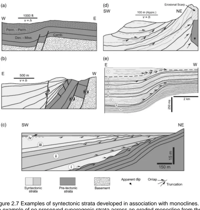
Cross-section A-A’ highlights the halokinetic growth geometry. Giles and Lawton (2002)...101 Figure 2.7 Examples of syntectonic strata developed in association with monoclines.

(a) An example of no preserved synorogenic strata across an eroded monocline from the Black Hills of the Western United States. (b)

Syntectonic strata geometries on the downthrown side of an early, normal-fault-related fold later dismembered by a through-going fault from the southern Rhine Graben. (c) An example from the eastern margin of the Gulf of Suez showing early syntectonic stratal relationships proposed for the normal-fault related South Baba monocline. (d) Another example from the eastern margin of the Gulf of Suez showing syntectonic stratal

relationships proposed for the normal-fault-related North Baba, syntectonic fold. (e) An example from the Atacama Basin of Northern Chile showing the syntectonic relationships across a monocline

associated with the Salar Fault. Patton (2004)………...102 Figure 2.8 (Top) Photomosaic of the growth strata assemblage from the Kaolin Wash

study area from Aschoff and Schmitt (2008). Photomosaic highlights the decrease in bedding dip and location of key surfaces. (Bottom) Line

sketch illustrates the geometry of the growth strata...103 Figure 2.9 Paleogeographic configuration of dextral transpressional collision (“run”) of

Baja BC micro plate and North America, resulting in the Laramide

Orogeny. Maxson and Tikoff (1996)...104 Figure 2.10 Schematic cross-section at approximately 40° N latitude of

lithospheric-scale buckling formed during the Laramide Orogeny. Wavelength of

folding is about 190 km. Tikoff and Maxson (2001)...105 Figure 2.11 Simplified cross-sections of tectonic models for the Front Range based on (A) vertical uplift, with gravity sliding of the western flank (Tweto (1980 (c)), (B) symmetric up-thrusts and positive strike-slip flower structures (Kelley and Chapin (1997)), (C) low-angle, symmetric thrust faulting in the central Front Range (Raynolds (1997)). Modified from Erslev et al. (2004)...106 Figure 2.12 Stratigraphic column of Maastrichtian to Eocene units deposited during the

Laramide Orogeny in the Denver Basin adjacent the central CFR.

Stratigraphic zone of interest is highlighted by red parentheses. Identified SU’s from three field locations (Wildcat Mtn., Perry Park/Statter Ranch,

(12)

and Air Force Academy) are also marked within the stratigraphic zone of interest. (Aschoff, 2010 personal communication)...108 Figure 2.13 Cross-section between two continuously cored wells (Kiowa core and

Castle Pines core) in the Denver Basin. Cross-section highlights the separation of the Dawson Formation (Late Cretaceous to Paleocene) into the D1 and D2 sequence by Raynolds (2002)...109 Figure 2.14 Chart from Thorson (2011) relating published nomenclature of the Denver

Basin Group from Thorson (2011) and Raynolds (1997, 2002) to common nomenclature...110 Figure 2.15 Facies diagram from Thorson (2011) for the Colorado Springs Area. This

diagram illustrates the relationship of the new formations presented by Thorson (2011)...111 Figure 2.16 Cross-section A-A’ showing geologic relationship within the study area at

the Air Force Academy from Kluth and Nelson (1988). “Star” symbols indicate the location of palynology samples from age dating. Wavy lines indicate identified angular unconformities. Kp- Pierre Shale, Kf- Fox Hill Sandstone, Kl- Laramie Formation, Tkd- Dawson Arkose...112 Figure 2.17 (A) Schematic drawing illustrating of the 3D growth-strata geometry of

SU’s along strike. The 3D growth strata geometry occurs when dip discordance decreases along strike within an SU. The green arrows highlight the “flat” portion of the geometry or the area with decreased dip discordance. The blue arrow highlights the “steeper” portion in the

geometry or an increase in dip discordance. (B) Arial photo of the growth strata exposure within the lower Dawson Formation at Perry Park/Statter Ranch with typical 3D in nature geometry. The arrows again highlight the “flattening” (green) and “steeper” (blue) parts of the 3D growth strata geometry in outcrop. Inserted map from Raynolds (2002). Inserted photo from Dechesne et al. (2011)...116 Figure 2.18 Photomosaic (A) and annotated photomosaic (B) of growth strata outcrop

in the lower Dawson Formation at the Air Force Academy near Colorado Springs, CO. This outcrop is the location of measured stratigraphic profiles AFB1 and AFB2. Inserted map from Raynolds (2002). High

resolution pdf included in Appendix A...117 Figure 2.19 Photomosaic (A) and annotated photomosaic (B) of growth strata outcrop

(13)

Figure 2.20 Annotated aerial photo of the growth strata exposure at Perry Park/ Statter Ranch. This is the location of measured stratigraphic profiles SR1 and SR2. Inserted map from Raynolds (2002)...121 Figure 2.21 Photomosaic (A) and annotated photomosaic (B) of Wildcat Tail and

Wildcat Mountain. This photo pictures measured stratigraphic profiles WT1, WT2, WT6, and WM1. Photo from Dr. Bruce Trudgill. Inserted map from Raynolds (2002)...122 Figure 2.22 Annotated aerial photo of the growth strata exposures at Wildcat Tail and

Wildcat Mountain. This is the location of measured stratigraphic profiles WT1, WT2, WT3, WT4, WT6, WM1, WM2. Inserted map from Raynolds (2002)...124 Figure 2.23 (A) Schematic drawings from Blair and McPherson (1994) showing the

features of the two types of alluvial fans (A) Debris-flow processes. (B) Sheet-flood processes. (B) Schematic drawing highlight the distinction between (A) truly distributary channels which are active simultaneously (the geomorphic definition), and (B) a radiating set of channels produced by sucessice nodal avulsions, but in which generally only one channel is active at one time (T1 then T2 then T3). Apparent channel bifurcations appear at the points of avulsion such as that labeled X, and at locations such as Y caused by the superposition of a channel over an older one. North and Warwick (2007). (C) Schematic drawing from DeCelles and Cavazza (1999) showing the main large-scale morphological and

depositional elements of a typical of a nonmarine foreland basin system. Drawing depicts two large fluvial megafans exiting from a gorge and meeting an axial fluvial trunk system...125 Figure 2.24 Schematic drawing showing unroofing of a foreland-type uplift and the

resulting sedimentation into the adjacent basin during fault-propagation folding. Drawing (A) shows development first of axial fluvial or lacustrine facies followed by coarse fan accumulation (B). DeCelles et al.

(1991)...133

Figure 2.25 Photos of lithofacies within Facies Association 1: Fluvial (confined). (A) Photo of lithofacies D with lenticular bed geometry (highlighted in blue) and ripple laminations and planar-tabular cross-stratification (highlighted in green). These characteristics are indicative of the fluvial (confined) facies association. (B) Photo of lithofacies B with characteristic lenticular bed geometry indicative of fluvial (confined) depositional systems...134 Figure 2.26 Photos of key sedimentary structures in outcrop. (A) Photo of horizontal

laminations from facies C at the Air Force Academy. Red arrow highlights the sedimentary structure. (B) Photo of ripple laminations from facies E at

(14)

the Air Force Academy. Red arrow highlights the sedimentary structure. (C) Photo of planar-tabular cross-stratification from facies H at Perry Park/Statter Ranch. Red arrow highlights the sedimentary structure. (D) Photo of trough cross-stratification from facies H at Perry Park/Statter Ranch. Red arrow highlights the sedimentary structure. (E) Photo of scour surface in facies E at the Air Force Academy. Red arrow highlights the sedimentary structure...135 Figure 2.27 Photos of all lithofacies from the fluvial (confined) lithofacies association

identified in outcrop of the lower Dawson Formation. Letter label indicates the lithofacies name and the color indicates the color used for that

lithofacies within the stratigraphic profiles and correlation...136 Figure 2.28 Photos of lithofacies within Facies Association 2: Unconfined

fluvial/megafan. (A) Photo of lithofacies H with planar-tabular cross-stratification and trough cross-cross-stratification highlighted in green. Large green line highlights a scour surface. (B) Photo of lithofacies H with tabular bed geometry highlighted in blue, indicative of the unconfined fluvial/megafan facies association...138 Figure 2.29 Photos of all lithofacies from the unconfined fluvial/megafan lithofacies

association identified in outcrop of the lower Dawson Formation. Letter label indicates the lithofacies name and the color indicates the color used for that lithofacies within the stratigraphic profiles and

correlation...139 Figure 2.30 Model from Miall (1985) of a proximal alluvial fan...141 Figure 2.31 Correlation of outcrop measured stratigraphic profiles of growth strata

exposures in the lower Dawson Formation along the CFR (S-N). High-resolution pdf included in Appendix A...142 Figure 2.32 Correlation of outcrop measured stratigraphic profiles of growth strata

exposures in the lower Dawson Formation at the Air Force Academy along the CFR (S-N). High-resolution pdf included in Appendix A...144 Figure 2.33 Correlation of outcrop measured stratigraphic profiles of growth strata

exposures in the lower Dawson Formation at the Perry Park/Statter Ranch along the CFR (S-N). High-resolution pdf included in Appendix A...146 Figure 2.34 Correlation of outcrop measured stratigraphic profiles of growth strata

(15)

Number of measurements are marked (N=). (A) AFB1 24 m (78 ft) (N=1). (B) AFB1 48 m (157 ft) (N=2). (C) AFB1 120 m (394 ft) (N=6). (D) AFB1 122 m (400 ft) (N=4). (E) AFB1 126 m (413 ft) (N=1). (F) AFB1 134 m (440 ft) (N=1). (G) AFB2 34 m (112 ft) (N=2)...152 Figure 2.36 Paleorose diagrams from paleocurrent measurements from the outcrops

at Perry Park/Statter Ranch. Number of measurements are marked (N=). Aerial photo highlights the area of outcrop exposure. (A) SR1 3 m (10 ft) (N=2). (B) SR1 8 m (26 ft), (N=2). (C) SR2 4 m (13 ft) (N=3)...153 Figure 2.37 Paleorose diagrams of paleocurrent data from the outcrop at Wildcat Tail.

Number of measurements are marked (N=). Aerial photo highlights the area of outcrop exposure. (A) WT1 3 m (10 ft) (N=7). (B) WT1 8 m (26 ft) (N=1). (C) WT2 3 m (10 ft) (N=3). (D) WT2 40 m (131 ft) (N=2). (E) WT4 18 m (59 ft) (N=2). (F) WT6 16 m (52 ft) (N=3)...154 Figure 2.38 Paleorose diagrams of paleocurrent measurements from the outcrop at

Wildcat Mountain. Number of measurements are marked (N=). Aerial photo highlights the area of outcrop exposure. (A) WM1 2 m (7 ft) (N=1). (B) WM1 50 m (164 ft) (N=1). (C) WM1 116 m (381 ft) (N=2). (D) WM2 20 m (67 ft) (N=1). (E) WM2 95 m (312 ft) (N=1). (F) WM2 128 m (420 ft) (N=1)...155 Figure 2.39 Schematic illustration from Aschoff and Schmitt (2008) showing the

differences between growth strata interpretations when (A) only traditional-type unconformities are identified and (B) when both traditional-traditional-type and subtle-type unconformities are identified...156 Figure 2.40 Correlation of well-log data (gamma-ray and resistivity curves) from the

CGS-CDWR along the CFR (S-N). High-resolution pdf included in

Appendix A. The datum for the well-log correlation is the base of the D1. The base of the D1 was chosen as the datum because it marks a change from more proximal fan advancement to fans within the lower Dawson Formation reaching further eastward within the basin (Dr. Peter Barkmann, personal communication 2013). This surface could be “a slight

unconformity at the active western basin boundary” (Dr. Peter Barkmann, personal communication 2013). The base of the D1 (datum) is identified in the resistivity logs as a shale break or low resistivity followed by a high in the resistivity log that marks the locations of the surface (Dr. Peter

Barkmann, personal communication 2013)...157 Figure 2.41 Palynomorph photos from Kluth and Nelson (1988) all at 630x

magnification. (A) Wodenhouseia spinata. (B) Aquilapollenites conatus. (C) Aquilapollenites delicates. (D) Libopollis. (E) Kurtsipites

(16)

Figure 2.42 Paleogeographic maps of the diachronous development of Laramide structures along the CFR and the development of the synorogenic sediment of the lower Dawson Formation through time. (A) Gravelly, braided fluvial (confined) deposits of the lower Dawson Formation/D1 sequence (Arapahoe Formation) begin to flow toward the Denver Basin near the Air Force Academy. Paleocurrent rose diagram is from

measurements taken from the Arapahoe Formation and indicate paleocurrent to the Northeast and the East. (B) Two periods of major uplift on emerging Laramide structures (red hill symbol) near the Air Force Academy. This interpretation is based on identified major (both traditional-type and subtle-traditional-type) SU’s in outcrop. The lower Dawson Formation depositional system is still fluvial (confined) but it is a combination of meandering and braided-type channels. The paleocurrent rose diagram are from measurements take from the fluvial (confined) lithofacies and has paleocurrent dominantly to the West. (C) The next major uplift on

Laramide structures near the Air Force Academy has propagated northward (from AFB1 to AFB3). The depositional system of the lower Dawson Formation is a unconfined fluvial/megafan with radiating pattern of paleocurrents to the Northeast and Southeast collected from the

unconfined fluvial/megafan lithofacies. (D) Structures begin to uplift in the Perry Park/Statter Ranch area. The depositional system here is

unconfined fluvial/megafan with no precursor fluvial (confined) deposition recognized. Paleocurrent has a radiating pattern from the Northeast to the Southeast and are collected from the unconfined fluvial/megafan

lithofacies. (E) Fluvial (confined) systems begin to emerge from the CFR and flow towards the Northeast at Wildcat Tail and Wildcat Mountain. At this time Laramide structure begin to propagate into the Wildcat

Mountain/Wildcat Tail area and uplift near Wildcat Tail. The paleocurrent rose diagram show paleocurrent to the Northeast and paleocurrent measurements were collected from the fluvial (confined) lithofacies. (F) Laramide structures propagate northward from Wildcat Tail to Wildcat Mountain (WM1). Two major uplift events are identified based on SU’s at the Wildcat Mountain outcrop (red hill symbol). The depositional system of the lower Dawson Formation at this time is an unconfined

fluvial/megafan. Paleocurrent measurements indicate a radiating pattern of paleocurrent with flow radiating from Northwest to Southeast. The paleocurrent measurements were collected from unconfined

fluvial/megafan lithofacies. (G) Laramide structures further propagate northward at Wildcat Mountain. The depositional system of the lower Dawson Formation is a unconfined fluvial/megafan. Paleocurrent measurements indicate a radiating pattern to paleoflow radiating from Northwest to Southeast. Paleocurrent measurements were collected from

(17)

Figure 3.1 Distrubution of key Laramide sedimentary basins and intervening uplifts in the Rocky Mountain region between central Montana and central New Mexico.(A) Map of the Western United States with the Franciscan

SaU-Sawatch; SCU-Sangre de Cristo; WiU-Wind River; WMU-Wet Mountains. Basins (B): BHB-Bighorn; GRB-Green River; PiB-Piceance; PRB-Powder River; RaB-Raton; WaB-Washakie; WRB-Wind River. Modified from Dickinson et al. (1988)...202 Figure 3.2 Stratigraphic column of Maastrichtian to Eocene units deposited during the

Laramide Orogeny in the Denver Basin adjacent to the central CFR. Stratigraphic zone of interest is highlighted by red parentheses. Identified SU’s from three field locations (Wildcat Mtn., Perry Park/Statter Ranch, and Air Force Academy) are also marked within the stratigraphic zone of

interest. (Aschoff, 2010 personal communication)...204 Figure 3.3 Diagram of unroofing of the southern Front Range in Colorado. (A) A time

of relative tectonic stability in central Colorado, (B) During early phases of Laramide deformation, grains were recycled out of Phanerozoic section, (C) Also during early Laramide deformation volcanism from the Colorado Mineral Belt contributed material to the Denver Basin, (D) By later stages of Laramide Deformation, most volcanic and sedimentary cover had been removed by earlier erosion, and synorogenic sediments in the basin were derived mainly from basement. Kelley (2002)...205 Figure 3.4 Chronostratigraphic chart of Upper Cretaceous to Paleogene rocks in

northeastern Utah and southwestern Wyoming. The focus of DeCelles and Cavazza (1999) is highlighted in red. DeCelles and Cavazza (1999)...207 Figure 3.5 (A) Conglomerate clast-count data from Hams Fork Conglomerate. Note

the relatively greater abundance of Paleozoic sandstone and carbonate clasts and lesser abundance of Proterozoic and lower Cambrian (Tintic) quartzite and Precambrian basement clasts in sections Northeast of Evanston, Wyoming. The bold dash line indicates the approximate boundary between the two petrofacies. (B) Paleogeographic map of the latest Cretaceous in the proximal part of the Cordilleran foreland basin system in northeastern Utah and southwestern Wyoming. The stippled areas represent fluvial megafans of the Hams Fork Conglomerate. The three principal source terranes for the Hams Fork Conglomerate are labeled-Willard thrust sheet, Wasatch anticlinorium, and the frontal ridges

(18)

of the Crawford and Absaroka thrust faults. The Cottonwood arch(~25 km South) may have also supplied detritus to the Hams Fork Conglomerate in the southwestern most part of the study area. Modified from DeCelles and Cavazza (1999)...208 Figure 3.6 Map of study areas in the Denver Basin. Map showing the basin extent,

paleomagnetism sample locations (purple triangles) from Hicks et al. (2003), and palynology sample locations (blue square) from this paper and Kluth and Nelson (1988). Geologic terminology is from Raynolds (2002). The formation of interest for this paper is the D1 sequence or lower

Dawson Formation (Late Cretaceous to Paleogene (TKd)). Basemap from Raynolds (2002)...210 Figure 3.7 QFL triplot diagram (Modified from Folk, 1968) of data from Wilson (2002).

The D1 sequence is highlighted in red. Modified from Wilson (2002)...213 Figure 3.8 (A)Chart of two major sedimentary components-chert and dolomite within

the Kiowa core. Note the three major spikes in total chert within the D1. (B) Chart of major feldspathic components- plagioclase, potassium

feldspar, and granitic fragments. Potassium feldspar is the most abundant in the samples from the D1 sequence. (C) Chart of volcanic components- silicic volcanics and basic volcanics. The largest pulse of silicic volcanic is in the upper portion of the D1 sequence Wilson (2002)...214

Figure 3.9 Dickinson QtFl Tectonic Setting Plot of Kiowa core samples data. The D1 sequence is highlighted in red. All of the samples from the D1 sequence plot in the transitional continental region of the plot. Modified from Wilson (2002)...217 Figure 3.10 (A) Chart of the four main provenance grain type categories illustrating

trends within the samples from the Kiowa core. Note the pulse of plutonic/high-grade metamorphics at the base of D1, the spike in

sedimentary type grains in the medial portion of D1, and the large spike in volcanic type grains in the lower and upper portions of D1. (B) Chart of the three major provenance grain type categories with the volcanic category removed. Again a pulse or spike in plutonic/high-grade metamorphics can be recognized at the base of D1, and a spike in sedimentary type grains within the medial portion of D1. Modified from Wilson (2002)...218 Figure 3.11 Chart of percentage of metamict, volcanic, and other as a function of

(19)

Figure 3.12 Triplot of quartzose components- plutonic/volcanic, bladed mineral inclusions, and chert. Quartz data from all four sample locations are

plotted...223 Figure 3.13 (A) Photo of typical metamorphic quartz in plain light (40x magnification)

(field of view ~ 0.5 mm) with characteristic bladed mineral inclusions. Red arrow highlights bladed mineral inclusion. (B) Photo of typical

metamorphic grain in cross-polarized light (40x magnification) (field of view ~ 0.5 mm) with characteristic bladed mineral inclusions. Red arrow highlights bladed mineral inclusion. (C) Photo of typical plutonic/volcanic quartz in plain light (10x magnification) (field of view ~ 3 mm). Red arrow highlights the quartz grain. (D) Photo of plutonic/volcanic quartz in cross-polarized light (10x magnification) (field of view ~ 3 mm) with characteristic “light to dark” or “quick” extinction. Red arrow highlights the quartz

grain...224 Figure 3.14 Triplot of plagioclase, alkali feldspar, and unassigned/altered feldspar data from all samples...225 Figure 3.15 Photos of the two typical type feldspars grains- alkali feldspar and

plagioclase feldspar. (A) Photo of an alkali feldspar grain in

cross-polarized light with distinct “tartan plaid” or grid twinning from sample CP 15 of the Castle Pines core (10x magnification) (field of view ~ 3 mm). Red arrow highlights the alkali feldspar grain. (B) Photo of a plagioclase

feldspar grain in cross-polarized light with distinct albite twinning from sample CP 8 of the Castle Pines core (10x magnification) (field of view ~ 3 mm). Red arrow highlights the plagioclase feldspar grain...226 Figure 3.16 Triplot of plutonic/volcanic, metamorphic, and sedimentary lithic grains for

all samples...228 Figure 3.17 Photos of example lithic-type grains (A) Photo of an igneous lithic grain

with visible phenocrysts in plain light from sample KC 16A from the Kiowa core (10x magnification) (field of view ~ 3 mm). Red arrow highlights the igneous grain. (B) Photo of the same igneous grain as photo (A) in cross-polarized light from sample KC 16A from the Kiowa core (10x

magnification) (field of view ~ 3 mm). Red arrow highlights grain. (C) Photo of a metamorphic lithic grain in plain light from sample CP 10 of the Castle Pines core (10x magnification) (field of view ~ 3 mm). Red arrow highlights the metamorphic grain. (D) Photo of the same metamorphic lithic grain as photo (C) in cross-polarized light from sample CP 10 of the Castle Pines core (10x magnification) (field of view ~ 3 mm). Red arrow highlights grains. (E) Photo of a sedimentary lithic grain in plain light from sample CP 15 of the Castle Pines core (10x magnification) (field of view ~ 3 mm). Red arrow highlights grain. (F) Photo of the same sedimentary grain as photo (E) in cross-polarized from sample CP15 of the Castle

(20)

Pines core (10x magnification) (field of view ~ 3 mm). Red arrow highlights grain. (G) Photo of unidentified heavy mineral lithic grain in plain light from sample CP5 of the Castle Pines core (10x magnification) (field of view ~ 3 mm). Red arrow highlights grain. (H) Photo of unidentified heavy mineral lithic grain in plain light from sample CP5 of the Castle Pines core (10x magnification) (field of view ~ 3 mm). Red arrow highlights grain...229 Figure 3.18 Photos of quartz grains from samples of the Kiowa core. (A) Photo of

sample 16A showing four quartz grains in plain light (10x magnification) (field of view ~ 3 mm). Red arrows highlight the quartz grains (B) Photo of sample 16A showing the same four quartz grains as photo (A) in cross-polarized light (10x magnification) (field of view ~ 3 mm). The “white” grain in the photo is a typical plutonic/volcanic category quartz grain. Red

arrows highlight the quartz grains (C) Photo of sample 24A showing five quartz grains in plain light (10x magnification) (field of view ~ 3 mm). Red arrow highlights the quartz grains (D) Photo of sample 24A showing the same five quartz grains as photo (C) but in cross-polarized light (10x magnification) (field of view ~ 3 mm). Red arrows highlight the five quartz grains...230 Figure 3.19 Photos of quartz grains from samples of the Castle Pines core. (A) Photo

of rutilated quartz (Qm) grain from sample CP15 in plain light (10x

magnification) (field of view ~ 3 mm). This is a typical metamorphic type quartz grain. Red arrow highlights the quartz grain. (B) Photo of same rutilated quartz (Qm) grain of photo (A) from sample CP15 in cross-polarized light (10x magnification) (field of view ~ 3 mm). Red arrow highlights the quartz grain (C) Photo of large quartz (Qm) grain from sample CP15 with large mineral inclusion or “negative crystal” in cross-polarized light (10x magnification) (field of view ~ 3 mm). Red arrow

indicates the quartz grain. (D) Photo of a microcrystalline quartz grain (Qp) from CP15 in cross-polarized light (10x magnification) (field of view ~ 3 mm). Red arrow highlights the microcrystalline quartz grain. (E) Photo of a lineated included quartz (Qm) grain from sample CP11 in cross-polarized light (10x magnification) (field of view ~ 3 mm). Red arrow highlights lineated included quartz grain. (F) Photo of quartz grain with abundant fluid inclusions in cross-polarized light (40x magnification) (field of view ~ 0.5 mm). Red arrow highlights quartz grain with the abundant fluid

inclusions...232 Figure 3.20 Photos of quartz grains from sample of a growth strata outcrop located at

the Air Force Academy (A) Photo of quartz grain from sample S1 in cross-polarized light with some fracturing and fluid inclusions (10x magnification)

(21)

sample S1 in cross-polarized light showing abundant bladed mineral

inclusions that are possibly mica (10x magnification) (field of view ~ 3 mm). Red arrow highlights quartz grain. (D) Photo of polycrystalline quartz (Qp) grain from sample S1 in cross-polarized light (10x magnification) (field of view ~ 3 mm). Red arrow highlights the quartz grain. (E) Photo of

polycrystalline quartz (Qp) grain from sample S2 in plain light (4x magnification) (field of view ~ 5 mm). Red arrow highlights the

polycrystalline quartz grain. (F) Photo of same polycrystalline quartz grain from photo (E) of sample S2 in cross-polarized light (4x magnification) (field of view ~ 5 mm). Red arrow highlights the polycrystalline quartz grain...233 Figure 3.21 Photos of a euhedral quartz grain from sample WM-1 taken from an

outcrop of growth strata at Wildcat Mountain. (A) Photo of euhedral quartz (Qm) grain in plain light (4x magnification) (field of view ~ 5 mm). Red arrow highlights quartz grain. (B) Photo of euhedral quartz grain in cross-polarized light (4x magnification) (field of view ~ 5 mm). Red arrow

highlights quartz grain...234 Figure 3.22 Photos of quartz grains from samples of Wildcat Mountain. (A) Photo of

microcrystalline quartz in plain light from sample WM 1 (10x magnification) (field of view ~ 3 mm). Red arrow highlights the grain. (B) Photo of the same microcrystalline (Qm ) quartz grain from photo (A) of sample WM 1 in cross-polarized light (10x magnification) (field of view ~ 3 mm). Red arrow highlights the grain. (C) Photo of monocrystalline quartz (Qm ) in plain light from sample WM 3 (10x magnification) (field of view ~ 3 mm). Red arrow highlights the grain. (D) Photo of the same monocrystalline quartz (Qm ) grain from photo (C) from sample WM 3 (10x magnification) (field of view ~ 3 mm). Red arrow highlights the grain. (E) Photo of monocrystalline quartz (Qm ) in plain light from sample WM 3 (10x magnification) (field of view ~ 3 mm). Red arrow highlights grain. (F) Photo of the same

monocrystalline quartz (Qm ) grain as photo (E) in cross-polarized light from sample WM 3 (10x magnification) (field of view ~ 3 mm). Red arrow highlights the grain...236 Figure 3.23 Photos of feldspar grains from samples of the Kiowa core. (A) Photo of an

alkali feldspar grain in plain light from sample KC 16A (4x magnification) (field of view ~ 5 mm). Red arrow highlights grain. (B) Photo the same alkali feldspar grain as photo (A) from KC 16A in cross-polarized light with visible “tartan plaid” or grid twinning (4x magnification) (field of view ~ 5 mm). Red arrow highlights the grain. (C) Photo of alkali feldspar grain in plain light from sample KC 38A (10x magnification) (field of view ~ 5 mm). Red arrow highlights the grain. (D) Photo of the same alkali feldspar grain as photo (C) from KC 38A in cross-polarized light with visible “spindle” twinning (10x magnification) (field of view ~ 3 mm). Red arrow highlights the grain. (E) Photo of two alkali feldspar grains in plain light from sample

(22)

KC 38A (4x magnification) (field of view ~ 3 mm). Red arrows highlight the grains. (F) Photo of the same two alkali feldspar grains as photo (E) from sample KC 38A in cross-polarized light (4x magnification) (field of view ~ 5 mm)...237 Figure 3.24 Schematic stratigraphic column of the Kiowa core (Raynolds, verbal

communication, 2012) with QFL triplot data from this paper. Two key sequence stratigraphic surfaces are also labeled- KaFS1 (Arapahoe Conglomerate flooding surface) and KaSB1 (Arapahoe Conglomerate Sequence Boundary)...239 Figure 3.25 Photos of feldspar grains from samples of the Castle Pines core. (A)

Photo of alkali feldspar grain from sample CP8 in plain light (10x

magnification) (field of view ~ 3 mm). (B) Photo of plagioclase feldspar grain from sample CP8 in cross-polarized light (10x magnification) (field of view ~ 3 mm). Red arrow highlights the feldspar grain with visible twinning. (C) Photo of alkali feldspar grain from sample CP11 in cross-polarized light (10x magnification) (field of view ~ 3 mm) with visible “spindle” extinction. Red arrow highlights feldspar grain. (D) (E) Photo of alkali feldspar grain from sample CP15 in plain light (10x magnification) (field of view ~ 3 mm). Red arrow highlights the feldspar grain. (F) Photo of same alkali feldspar grain from sample CP15 in cross-polarized light (10x

magnification) (field of view ~ 3 mm). “Tartan plaid” or grid twinning visible. Red arrow highlights feldspar grain...241 Figure 3.26 Schematic stratigraphic column of the Castle Pines core (Raynolds et. al

2001) with QFL triplot data of each sample from this paper. Two key sequence stratigraphic surfaces are also labeled- KaFS1 (Arapahoe Conglomerate flooding surface) and KaSB1 (Arapahoe Conglomerate Sequence Boundary)...242 Figure 3.27 Photos of feldspar grains from samples of the Air Force Academy

outcrops with the three classification types shown- alkali feldspar, plagioclase feldspar, and unassigned altered. (A) Photo of an alkali feldspar grain from sample S 1 in plain light (10x magnification) (field of view ~ 3 mm). Red arrow highlights the alkali feldspar grain. (B) Photo of the same alkali feldspar grain as photo (A) from sample S 1 in cross-polarized light (10x magnification) (field of view ~ 3 mm). “Tartan plaid” or grid twinning visible. Red arrow highlights alkali feldspar grain. (C) Photo of an alkali feldspar grain from sample S 1 in plain light (10x magnification) (field of view ~ 3 mm). Red arrow highlights alkali feldspar grain. (D) Photo of the same alkali feldspar grain as photo (C) from sample S 1 in

(23)

cross-highlights the altered feldspar grain. (F) Photo of alkali feldspar grain from sample S 2 in cross-polarized light (10x magnification) (field of view ~ 3 mm). Red arrow highlights the alkali feldspar grain…………...244 Figure 3.28 Stratigraphic column of the Air Force Academy growth strata outcrop with

QFL triplot data of each sample. Two key sequence stratigraphic surfaces are also labeled- KaFS1 (Arapahoe Conglomerate flooding surface) and KaSB1 (Arapahoe Conglomerate Sequence Boundary)...246 Figure 3.29 Photos of feldspar grains from samples of Wildcat Mountain. (A) Photo of

an alkali feldspar grain in plain light from sample WM 1 (10x magnification) (field of view ~ 3 mm). Red arrow highlights the grain. (B) Photo of the same alkali feldspar grain as photo (A) from sample WM 1 in

cross-polarized light with visible “tartan plaid” or grid twinning (10x magnification) (field of view ~ 3 mm). Red arrow highlights the grain. (C) Photo of an alkali feldspar grain in plain light from sample WM 1 (10x magnification) (field of view ~ 3 mm). Red arrow highlights the grain. (D) Photo of the same alkali feldspar grain as photo (C) from sample WM 1 in

cross-polarized light with visible “tartan plaid” or grid twinning (10x magnification) (field of view ~ 3 mm). Red arrow highlights the grain. (E) Photo of alkali feldspar grain from sample WM 3 in cross-polarized light with visible “tartan plaid” or grid twinning (10x magnification) (field of view ~ 3 mm). Red arrow highlights the grain. (F) Photo of plagioclase feldspar grain from sample WM 3 in cross-polarized light (4x magnification) (field of view ~ 5 mm). Red arrow highlights the grain...247 Figure 3.30 Stratigraphic column of the Wildcat Mountain growth strata outcrop with

QFL triplot data of each sample. Two key sequence stratigraphic surfaces are also labeled- KaFS1 (Arapahoe Conglomerate flooding surface) and KaSB1 (Arapahoe Conglomerate Sequence Boundary)...248 Figure 3.31 Photos of lithic grains from samples of the Kiowa core. (A) Photo of

igneous lithic grain from sample KC 38A in plain light (4x magnification) (field of view ~ 5 mm). Red arrow highlights the grain. (B) Photo of the same igneous lithic grain as photo (A) from sample KC 38A in cross-polarized light with visible phenocrysts (4x magnification) (field of view ~ 5 mm). Red arrow highlights the grain. (C) Photo of an igneous lithic grain from sample KC 16A in plain light (10x magnification) ((field of view ~ 3 mm). Red arrow highlights the grain. (D) Photo of the same igneous lithic grain as photo (C) from sample KC 16A in cross-polarized light with visible phenocrysts (10x magnification) (field of view ~ 3 mm). Red arrow

highlights the grain. (E) Photo of a metamorphic lithic grain from sample KC 16A in plain light (10x magnification) (field of view ~ 3 mm). Red arrow highlights the grain. (F) Photo of the same metamorphic lithic grain as photo (E) from sample KC 16A in cross-polarized light (10x magnification) (field of view ~ 3 mm). Red arrow highlights the grain...250

(24)

Figure 3.32 Photos of lithic grains from samples of the Castle Pines core. (A) Photo of a zircon grain from sample CP 11 in plain light (10x magnification) (field of view ~ 3 mm). Red arrow highlights the grain. (B) Photo of the same zircon grain from photo (A) from sample CP 11 in cross-polarized light (10x magnification) (field of view ~ 3 mm). Red arrow highlights the grain. (C) Photo of sedimentary lithic grain from sample CP 15 in plain light (10x magnification) (field of view ~ 3 mm). Red arrow highlights the grain. (D) Photo of the same sedimentary lithic grain as photo (C) from sample CP 15 in cross-polarized light (10x magnification) (field of view ~ 3 mm). Red arrow highlights the grain. (E) Photo of unidentified heavy mineral lithic grain from sample CP 5 in plain light (10x magnification) (field of view ~ 3 mm). Red arrow highlights the grain. (F) Photo of the same unidentified heavy mineral grain as photo (E) from sample CP 5 in cross-polarized light (10x magnification) (field of view ~ 3 mm). Red arrow highlights the

grain...252 Figure 3.33 Photos of examples of unidentified lithic type grains. (A) Photo of an

unidentified grain from sample CP 15 of the Castle Pines core in plain light with visible alteration rim (10x magnification) (field of view ~ 3 mm). Red arrow highlights the unidentified grain. (B) Photo of the same unidentified grain from photo (A) from sample CP 15 of the Castle Pines core in cross-polarized light (10x magnification) (field of view ~ 3 mm). Visible alteration rim with dark center. Red arrow highlights unidentified grain. (C) Photo of an unidentified lithic grain or heavy mineral grain from sample CP 5 of the Castle Pines core in plain light (10x magnification) (field of view ~ 3 mm). Red arrow highlights unidentified grain...253 Figure 3.34 Modified Folk (1968) triplot diagram of QFL data from both Wilson (2002)

and this paper. Wilson (2002) D1 data points are highlighted in red. Data points from this paper are explained in the table to the right...255 Figure 3.35 Dickinson QtFL triplot for Tectonic Setting with data from both Wilson

(2002) and this paper. Wilson (2002) data points for the D1 are highlighted in red and data points from this paper are explained to the left...256 Figure 3.36 Map of Denver Basin with noted sample sites of this paper. Extent of

fluvial megafans within the D1 are dashed in orange, and are based on two distinct petrofacies identified in this paper. Basemap is from Raynolds (2002)...257 Figure 4.1 Map of study areas in the Denver Basin. Map showing the basin extent,

(25)

The formation of interest is the D1 sequence or lower Dawson Formation (Late Cretaceous to Paleogene (TKd)). Basemap from Raynolds

(2002)...271 Figure 4.2 Correlation of outcrop measured stratigraphic profiles of growth strata

exposures in the lower Dawson Formation along the CFR (S-N). High-resolution pdf included in Appendix A...272 Figure 4.3 Correlation of outcrop measured stratigraphic profiles of growth strata

exposures in the lower Dawson Formation at the Air Force Academy along the CFR (S-N). High-resolution pdf included in Appendix A...274 Figure 4.4 Correlation of outcrop measured stratigraphic profiles of growth strata

exposures in the lower Dawson Formation at the Perry Park/Statter Ranch along the CFR (S-N). High-resolution pdf included in Appendix A...276 Figure 4.5 Correlation of outcrop measured stratigraphic profiles of growth strata

exposures in the lower Dawson Formation at Wildcat Mountain along the CFR (S-N). High-resolution pdf included in Appendix A...278 Figure 4.6 Paleogeographic maps of the diachronous development of Laramide

structures along the CFR and the development of the synorogenic sediment of the lower Dawson Formation through time. (A) Gravelly, braided fluvial (confined) deposits of the lower Dawson Formation/D1 sequence (Arapahoe Formation) begin to flow toward the Denver Basin near the Air Force Academy. Paleocurrent rose diagram is from

measurements taken from the Arapahoe Formation and indicate paleocurrent to the Northeast and the East. (B) Two periods of major uplift on emerging Laramide structures (red hill symbol) near the Air Force Academy. This interpretation is based on identified major (both traditional-type and subtle-traditional-type) SU’s in outcrop. The lower Dawson Formation depositional system is still fluvial (confined) but it is a combination of meandering and braided-type channels. The paleocurrent rose diagram are from measurements take from the fluvial (confined) lithofacies and has paleocurrent dominantly to the West. (C) The next major uplift on

Laramide structures near the Air Force Academy has propagated northward (from AFB1 to AFB3). The depositional system of the lower Dawson Formation is a unconfined fluvial/megafan with radiating pattern of paleocurrents to the Northeast and Southeast collected from the

unconfined fluvial/megafan lithofacies. (D) Structures begin to uplift in the Perry Park/Statter Ranch area. The depositional system here is

unconfined fluvial/megafan with no precursor fluvial (confined) deposition recognized. Paleocurrent has a radiating pattern from the Northeast to the Southeast and are collected from the unconfined fluvial/megafan

lithofacies. (E) Fluvial (confined) systems begin to emerge from the CFR and flow towards the Northeast at Wildcat Tail and Wildcat Mountain. At

(26)

this time Laramide structure begin to propagate into the Wildcat

Mountain/Wildcat Tail area and uplift near Wildcat Tail. The paleocurrent rose diagram show paleocurrent to the Northeast and paleocurrent measurements were collected from the fluvial (confined) lithofacies. (F) Laramide structures propagate northward from Wildcat Tail to Wildcat Mountain (WM1). Two major uplift events are identified based on SU’s at Wildcat Mountain (red hill symbol). The depositional system of the lower Dawson Formation at this time is an unconfined fluvial/megafan.

Paleocurrent measurements indicate a radiating pattern of paleocurrent with flow radiating from Northwest to Southeast. The paleocurrent

measurements were collected from unconfined fluvial/megafan lithofacies. (G) Laramide structures further propagate northward at Wildcat Mountain. The depositional system of the lower Dawson Formation is a unconfined fluvial/megafan. Paleocurrent measurements indicate a radiating pattern to paleoflow radiating from Northwest to Southeast. Paleocurrent

measurements were collected from the unconfined fluvial/megafan

lithofacies...280 Figure 4.7 Map of Denver Basin with noted sample sites of this paper. Extent of

fluvial megafans within the D1 are dashed in orange, and are based on two distinct petrofacies identified in this paper. Modified Basemap from Raynolds (2002)...284

(27)

LIST OF TABLES

Table 2.1 Table of identified SU’s (syntectonic unconformities) at all three

stratigraphic profiles at the Air Force Academy. Table includes the location, dip discordance, and facies it was located. The SU’s highlighted in yellow are major (both traditional-type and subtle-type) SU’s representing uplift events during the Laramide Orogeny in the eastern, central CFR

region...113 Table 2.2 Table of identified SU’s (syntectonic unconformities) at two stratigraphic

profiles at the Perry Park/Statter Ranch. Table includes the location, dip discordance, and facies it was located. The SU’s highlighted in yellow are major (both traditional-type and subtle-type) SU’s representing uplift events during the Laramide Orogeny in the eastern, central CFR

region ...114 Table 2.3 Table of identified SU’s (syntectonic unconformities) at all seven

stratigraphic profiles at Wildcat Mountain and Wildcat Tail. Table includes the location, dip discordance, and facies it was located. The SU’s

highlighted in yellow are major (both traditional-type and subtle-type) SU’s representing uplift events during the Laramide Orogeny in the central CFR region ...115 Table 2.4 Table of facies associations with descriptions and interpretations...127 Table 2.5 Table of facies descriptions, depositional process, and depositional

environment for the facies in association 2: fluvial (confined)

deposit...129 Table 2.6 Table of facies descriptions, depositional process, and depositional

environment for facies in association 1: unconfined fluvial/megafan

deposit...131 Table 2.7 Table of paleocurrent measurements collected from growth strata

outcrops...150 Table 2.8 Table of palynology analysis data from outcrop samples...159 Table 3.1 Table of QFL percentages from samples of the Kiowa core for the D2

sequence, D1 sequence, Laramie Formation, Fox Hill Sandstone, and Pierre Shale. Wilson (2002)...211 Table 3.2 Table of provenance components with five major categories for the Kiowa

(28)

Table 3.3 (A) Table of average quartz, feldspar, and lithic percentages for the four sample locations and an average for the D1 sequence. Percentages based on total amount of framework grains. Table on the left is modified from Wilson (2002) and includes QFL data for the D1 sequence from the Kiowa core. (continued) (B) Table of average quartz, feldspar, and lithic percentages and an average percentage for the D1 sequence..

Percentages based on total quartz, feldspar, and lithic grains. Table on the left is modified from Wilson (2002) and includes QFL data for the D1 sequence from the Kiowa core...221,222 Table 3.4 Percentages of each Qm type and each Q p type for each sample...231 Table 3.5 Percentages of feldspar type for each sample...238 Table 3.6 Percentages of each type of lithic grain- igneous, volcanic, metamorphic,

sedimentary, and unidentified for each sample...251 Table 4.1 (A) Table of average quartz, feldspar, and lithic percentages for the four

sample locations and an average for the D1 sequence. Percentages based on total amount of framework grains. Table on the left is modified from Wilson (2002) and includes QFL data for the D1 sequence from the Kiowa core.(continued) (B) Table of average quartz, feldspar, and lithic percentages and an average percentage for the D1 sequence.

Percentages based on total quartz, feldspar, and lithic grains. Table on the left is modified from Wilson (2002) and includes QFL data for the D1

(29)

ACKNOWLEDGMENTS

This work was funded by the Rocky Mountain Association of Geologist Babcock Scholarship, the Wyoming Geological Association Dr. J. Love Field Geology

Scholarship, the SEPM Student Research Fund, and the Colorado School of Mines Geology and Geological Engineering Department Nikki Hemmesch Fellowship. I would like to thank Michele Wiechman, Zane Houston, Erich Heydweiller, Matthew Lewis, and Patrick Geesaman for their assistance in the field. I would also like to thank Dr. Peter Barkmann and the Colorado Geological Society for providing data and support for this project. I would like to extend thanks to Dr. Bob Raynolds and the Denver Museum of Nature and Science for petrographic thin sections for this project and insight into the lower Dawson Formation. Thanks also goes to the Department of Wildlife and Fisheries at the U.S. Air Force Academy, Dr. Brian Mihlbachler and Greg Speights for sponsoring all my visit to the Air Force Academy. I would also like to thank Kamil Tazi and Fred and Diane LaRoche for granting me access to their property and their support.

I would like to thank Dr. Aschoff and my committee- Dr. Bruce Trudgill and Dr. Chuck Kluth for sharing their knowledge of the Denver Basin with me.

(30)

For my parents, Jeff and Kerri

Without you this would not be possible

and

My brother, Jake My best friend

(31)

CHAPTER 1 INTRODUCTION

This chapter focuses on providing the context and reasoning behind this thesis. The purpose of this work is presented and its importance is supported by the lack of agreement on kinematic models for the Laramide Orogeny along the central Colorado Front Range (CFR), and the need for an integrated stratigraphic approach to this problem.

1.1 PURPOSE OF STUDY

Growth strata can provide valuable information that can unlock the timing and development of structures along strike of the CFR. The number of syntectonic unconformities and their amount of discordance within growth strata indicate the number of phases when uplift exceeded sedimentation. Growth-strata sequences and their constituent unconformities on the eastern CFR will decipher the location and relative timing of local uplifts that composed the eastern CFR front during the Laramide Orogeny (sensu Riba (1978), Verges et al. (2002), Patton (2004), Aschoff and Schmitt (2008)). Along-strike correlation of the syntectonic unconformities supplemented by published chronostratigraphic data provides the relative timing of uplift at each location, and reveals the linking of uplifts through time. Understanding how these basinward thrust structures developed along the eastern, central CFR provides insight to the over mechanism of Laramide-style uplift, and can provide clarity to the four models proposed for the CFR (Figure 1.1). The development of thrust faulting in narrow bands on each

(32)

side of the CFR and how significant these faults are compared to strike-slip motion is still contested (Kelley and Chapin 1997).

Prior to this paper, only one growth strata outcrops had been documented along the eastern CFR due to their low preservation potential, and only one of these has been reported (Kluth and Nelson 1988). This paper highlights two additional exposures that were identified at the Air Force Academy in Colorado Springs, CO. Other well-exposed outcrops are located near Perry Park, CO and at Wildcat Mountain in Sedalia, CO (Figure 1.2). This paper evaluates whether (1) basinward-directed thrust faults develop as a series of isolated fault related structures that parallel the main S-N proto-Colorado Front Range (2) did the linking of basinward-directed thrust faults laterally (i.e., transfer or transverse zones) control the position of coarse-grained, locally distinct clastic tongues within the lower Dawson Formation (D1 sequence)?

1.2 PREVIOUS CFR MODELS OF LARAMIDE UPLIFT

The CFR is one of the most striking features in Western North America, forming the sharp boundary between the highest peaks of the Rockies and the Great Plains. Loading of the crust by the CFR uplift caused crustal flexure that formed the adjacent Denver Basin, where important oil/gas reservoirs and water aquifers form part of the basin-fill (Figure 1.1). Despite the importance of the CFR and its associated basin for natural resources, there were just a handful of studies that have interrogated the close relationship between structural development and basin formation. One of the key remaining questions regarding the CFR is what is how frontal thrust developed along

(33)

1.2.1 GEOLOGICAL CONTEXT

The term “Laramide” traditionally refers to tectonic movements of the latest Cretaceous and early Tertiary time in the western Cordillera Foreland Basin (Dickinson et al. 1988). Laramide-style uplifts are thick-skinned, basement-cored uplifts with

intervening sediment-filled foreland basins that formed during the time-transgressive Laramide Orogeny (Dickinson et al. 1988). The Laramie Orogeny is the result of deformation caused by the subduction of the shallow Farallon plate and its North-Northeast (oblique) trajectory beneath the craton from Southwest Arizona through Wyoming (Saleeby 2003). In the central Rocky Mountain region, Laramide-style uplifts segregated the foreland basin into discrete local basins. These emerging basement-cored uplifts eventually became the source of orogenic sediment within the localized basins (Figure 1.1) (Dickinson et al. 1988).

The Laramide Orogeny occurred during the Late Cretaceous-Early Tertiary on the site of the Late Paleozoic basement-cored uplift (Kluth 1997). The CFR is one of the Laramide-style uplifts in the Rocky Mountain region, and is 180 miles long and 40 miles wide (Sonnenberg and Boylard 1997). The basic tectonic framework set forth in the central CFR area during the Precambrian effected later structural features such as Laramide uplift (sensu Badgley 1960). The dominant trend of the three fault trends contained in the Precambrian rocks is North-Northwest, and the influence of this dominant trend within the Precambrian rocks can be seen on younger structures (Sonnenberg and Boylard 1997).

Raynolds (1997) states that uplift of the central Front Range was a subset of the regional basement-involved compressive and transpressive orogenic forces responsible

(34)

for the deformation of much of the uplift in Montana, Wyoming, Utah, and Colorado. The Laramide uplift or deformation on the eastern side of the Front Range in Colorado is composed of West-Southwest and East-Northeast dipping thrust and reverse faults (Erslev and Selvig 1997). The along-strike style of deformation changes along the length of basement-cored uplifts despite relatively uniform basement rock (Erslev and Selvig 1997).

In cross-sectional view, the basin is asymmetric, with its deeper portion to the West suggesting a flexural subsidence mechanism for the Denver Basin (Sonnenberg and Boylard 1997). The sedimentary record of the Laramide Orogeny is contained within the Arapahoe (~68-67 Ma), Denver 63.5 Ma), and Dawson Formation (~67-63.5 Ma) (Figure 1.3). The Dawson Formation is predominantly alluvial arkosic

conglomerates indicating a nearby western highland with enough relief and erosion to shed abundant Precambrian granitic debris (Grose 1960). Adjacent to the fault contact, the Dawson Formation is locally folded and overturned (Grose 1960). Raynolds (1997) postulated that strata deposited during the Laramide Orogeny record two discrete episodes of uplift on the Front Range bounding thrust faults.

1.2.2 ORIGINS OF THE LARAMIDE OROGENY

Prucha et al. (1965) first investigated the origin of basement-cored uplifts in the Rocky Mountain region using examples from Montana, Wyoming, Colorado, and New Mexico. Based on experimental rock deformation data, Prucha et al. (1965) suggested that Laramide deformation was due to basement block faulting bounded by upthrust

(35)

Orogeny based on the correlation in both space and time between the magmatic null in the western Cordillera and the classic Laramide Orogeny in the eastern Cordillera. Moreover, Dickinson and Snyder (1978) noted that orogenies are classified as arc, collision, or transform orogenies, but the Laramide Orogeny does not fit into any of these models. Comparing foreland flow speed and direction with the known motion of the Kula and Farallon plates confirms that the Laramide Orogeny had a different

mechanism than the Sevier Orogeny: it was driven by basal traction during an interval of horizontal subduction (i.e., flat-slab) not by edge forces due to coastal subduction or spreading of the western Cordillera or by accretion of terranes to the coast (Bird 1998).

Research by Maxson and Tikoff (1996), Tikoff and Maxson (2001), and Saleeby (2003) provided alternative models for Laramide-style deformation in the Rocky

Mountain region. The first suggested model by Maxson and Tikoff (1996) is a “hit-and-run” model for the Laramide Orogeny. Maxson and Tikoff (1996) argue that the scale of the tectonic style resembles a collision-type, but the collider is not preserved at this latitude. They provide the terranes of western British Columbia and Southeast Alaska as the collider (the “hit”). The western British Columbia and Southeast Alaska collider subsequently translated northward during oblique convergence (the “run”) to its present latitude (94 Ma and ca. 40 Ma.)(Figure 1.4) (Maxson and Tikoff 1996). The “hit-and-run” movement of these terranes are spatially and temporally coincident with the

development of the Laramide Orogeny (80 to 45 Ma) (Maxson and Tikoff 1996). The next model suggested by Tikoff and Maxson (2001) is lithospheric buckling as the primary cause of the Laramide-style uplifts; theirs is consistent with the wavelength of arches in the Western United States but does not explain the wide range of structural

(36)

styles observed in the Laramide province. Saleeby (2003) states that the subduction of a shallow slab portion of the Farallon plate can be correlated to plate edge and interior Laramide deformation. Saleeby (2003) provides a modern analogue of this shallow slab subduction causing interior deformation is the Juan Fernandez Rise subduction beneath the southern Andes and the adjacent Sierra Pampeanas foreland thrust belt.

1.2.3 KINEMATIC MODELS OF THE COLORADO FRONT RANGE

Three kinematic models were proposed for the Laramide Orogeny in the central CFR (Figure 1.6). The first model is vertical uplift with large vertical faults bounding the western and eastern sides of the central CFR (Figure 1.6 (A)). Tweto (1980c) argues that arching and up faulting are the mechanism of Laramide-style uplift along the CFR, because the opposing reverse and thrust faults on each side of the CFR can be

interpreted as near-surface expressions of steep faults (Figure 1.6 (A)) (Sonnenberg and Boylard 1997). The second model is horizontal/lateral compression. The

horizontal/lateral compression kinematic hypothesis is supported by evidence of bounding thrust faults that bound both the western and eastern edges of the central CFR. An upthrust and strike-slip flower structure model has also been used to support the horizontal/lateral compression hypothesis (Figure 1.6 (B)) (Erslev et. al 2004, Kelley and Chapin 1997). The theory of horizontal compression gained ground with advances in seismic imaging in the 1980’s, which supports shortening of the CFR (sensu

Sonnenberg and Boylard 1997). The third kinematic model is low-angle, symmetric thrust faulting (Figure 1.6 (C)) (Raynolds 1997). The third model has the low-angle,

(37)

debated (Erslev 1991, Erslev et al. 2004, Erslev 2005, Kelley and Chapin 1997, and Raynolds 1997).

1.3 LARAMIDE-STRUCTURES AND GROWTH STRATA

Growth strata associated with Laramide structures can provide insight on the timing and the development and propagation of thrust-bounding faults. Laramide-style structures and their development were documented, but the use of growth strata has been under utilized throughout the literature. Often growth strata sequences are identified but never analyzed in detail. An example of this under utilization is the identification of growth strata packages within a Paleocene synorogenic conglomerate juxtaposed to the Beartooth Range, Wyoming (DeCelles et. al 1989). The Beartooth Range is the result of the Laramide Orogeny and contains Laramide-style structures. Facies and provenance analysis was conducted on the Paleocene conglomerate, but no analysis of the growth strata geometries, syntectonic unconformities, or analysis of lateral linking of those syntectonic unconformities (DeCelles et al. 1989). Provenance analysis showed the presence of an unroofing signal produced from the removal of Upper Cretaceous through Precambrian section of the eastern Beartooth Range (DeCelles et. al 1989). If the facies analysis and provenance analysis were combined with growth strata analysis then a more detailed development of the Laramide

structures within the Beartooth Range could be produced. This paper integrates both examination of external growth strata geometries with detailed growth strata

(38)

1.4 UNROOFING SIGNALS IN THE DENVER BASIN

Variations in provenance within the lower Dawson Formation in the Denver Basin have implications on fluvial megafan development during the Laramide Orogeny.

Variations, like grain-type, can be used to establish petrofacies for the emerging fluvial megafans within the lower Dawson Formation. Identification of trends within the grain-type constituents can also reveal an unroofing signal that developed in response to the removal of Phanerozoic cover and Precambrian basement due to emerging Laramide structures.

Unroofing sequences show provenance variations through the section as an uplift or tectonic event occurs during the deposition. The first “source” deposited would be the first unit to be exposed during an uplift or the youngest unit in the sequence, resulting in an inverted stratigraphy of the source (Figure 1.7) (Wilson 2002). The stages of unroofing during the Laramide Orogeny started with the Phanerozoic cover and ended with the Precambrian basement (Figure 1.7). The synorogenic deposits of the Laramide Orogeny include the Arapahoe, Dawson (D1 and D2 sequences

(Raynolds 1997, 2002)), and the Denver Formations (Figure 1.3). Identifying unroofing sequences along strike and comparing the development of the unroofing sequence between outcrops of the lower Dawson Formation (D1 sequence) can support whether the development was synchronous or diachronous along strike. The data along strike (near the CFR) can also be compared to the unroofing sequence within the basin.