A disaggregate bundle method for train timetabling problems

A disaggregate bundle method for train

timetabling problems

Abderrahman Ait Ali, Per Olov Lindberg, Jonas Eliasson, Jan-Eric Nilsson and

Anders Peterson

The self-archived postprint version of this journal article is available at Linköping

University Institutional Repository (DiVA):

http://urn.kb.se/resolve?urn=urn:nbn:se:liu:diva-165781

N.B.: When citing this work, cite the original publication.

Ait Ali, A., Lindberg, P. O., Eliasson, J., Nilsson, J., Peterson, A., (2020), A disaggregate bundle method for train timetabling problems, Journal of Rail Transport Planning & Management. https://doi.org/10.1016/j.jrtpm.2020.100200

Original publication available at:

https://doi.org/10.1016/j.jrtpm.2020.100200

Copyright: Elsevier

A Disaggregate Bundle Method for Train

Timetabling Problems

Abderrahman Ait-Ali

_{, Per Olov Lindberg}

_{, Jonas Eliasson}

_,

Jan-Eric Nilsson

_{and Anders Peterson}

1 _{Swedish National Road and Transport Research Institute (VTI), Malvinas väg 6, SE-114} 28 Stockholm, Sweden

2 _{Department of Science and Technology, Linköping University} * _{E-mail: abderrahman.ait.ali@vti.se, phone: +46 (0) 8 555 367 81}

Abstract

The train timetabling problem (TTP) consists of finding a feasible timetable for a number of trains which minimises some objective function, e.g., sum of running times or deviations from ideal departure times. One solution approach is to solve the dual problem of the TTP using so-called bundle methods. This paper presents a new bundle method that uses disaggregate data, as opposed to the standard bundle method which in a certain sense relies on aggregate data. We compare the disaggregate and aggregate methods on realistic train timetabling scenarios from the Iron Ore line in Northern Sweden. Numerical results indicate that the proposed disaggregate method reaches better solutions faster than the standard aggregate approach.

Keywords

Train timetabling; disaggregation; bundle methods; lagrangian relaxation; mathematical programming.

1 Introduction

The train timetabling problem (TTP) refers to finding a feasible train timetable that minimises some objective functions. Such a timetable specifies where each train is located at given times over a certain period and is often presented as a graphical space-time diagram. That the timetable is feasible means that it should be free of conflicts between trains and satisfy certain functional constraints given by the railway system, such as the track capacity resulting from the physical infrastructure and the signalling system.

Train path requests (e.g., ideal departure time, latest arrival time and stopping stations) are received from the train operator(s). An infrastructure manager is tasked to produce a feasible train timetable that maximises a certain total objective function (e.g., total utility) based on the received train path requests. Due to network capacity restrictions, certain path requests are sometimes adjusted or rejected (i.e., not included in the final timetable).

TTPs are often formulated as mathematical programs, e.g., Integer Linear Programs (ILPs) or Mixed Integer Programs (MIPs). Solving such models, i.e., finding an optimal (or good quality) solution, is not always easy. Solution methods that make use of simplifications or heuristics are often needed to make the computational solution time realistic and tractable.

Relaxation methods, such as lagrangian relaxation, have been widely used as solution methods for solving the TTP models. In these solution methods, the (easier) dual program

resulting from the relaxation becomes the focus rather than the (harder) TTP program (called primal). Bundle methods are often used to solve the dual programs resulting from lagrangian relaxation of TTP models. For instance, Brännlund et al. (1998) adopted a standard bundle method where aggregate information from all the train requests are used to solve the dual problem arising from lagrangian relaxation of a discrete-time and space formulation of TTP.

In the present paper, we propose an improved variant of bundle method using a disaggregate approach where the optimisation is performed with separate dual information for each train request. The aim of the paper is to derive the novel approach (called

disaggregate) based on the same TTP model by Brännlund et al. (1998), and study its

performances on some real-world timetabling scenarios. We show that the proposed approach results in substantial reductions in computation times, up to 45 % (excluding the initialisation phase), compared to the standard bundle method.

In the following section, several related works are reviewed and compared to this paper. The mathematical program of the TTP is formulated in section 3. We derive in section 4 the two solution methods, i.e., aggregate and disaggregate approach. In section 5, we test the two approaches and compare their performances on realistic train timetabling scenarios from the single-track Iron Ore railway line (Malmbanan) in Northern Sweden. Section 6 concludes the paper.

2 Related Work

The research literature related to the topic is rich. Many research papers focused on modelling TTP or on solving it, while others treated both. In this section, we present some of the related work from the research literature.

TTPs can be modelled using alternative basic formulations leading to various mathematical programs. The main variables, i.e., space and time, can be discretised and lead to ILPs (Yue et al., 2016) or continuous and lead to MILPs such as Bach et al. (2018) and Forsgren et al. (2013). Most TTP models are linear but they can also be nonlinear if the constraints or objective function include a nonlinear term (Xu et al., 2014). Some TTP models focused on single track lines (Brännlund et al., 1998) whereas others on more general railway networks (Meng and Zhou, 2014). In addition to standard off-line TTPs, certain models are also used for real time (online) timetabling under disturbances, i.e., operational planning such as the models by Törnquist and Persson (2007), Törnquist (2012) or Quaglietta et al. (2016). The final timetables can have a specific format, e.g., cyclic as in Zhang et al. (2019b) or periodic as in Jamili et al. (2012).

Different TTP models include various types of constraints and variables. Track occupancy constraints and blocking rules are particularly important for single track. Traditionally, these constraints are included in the ILP using big-M techniques. Alternatively, Meng and Zhou (2014) introduced cumulative flow variables. Instead of using standard space and time variables (i.e., departure or arrival time at specific stations as in time–space network modelling framework), Cacchiani et al. (2008) used variables where each variable corresponds to the timetable of a train, i.e., all the train path from origin to destination. Additional constraints such as maintenance can also be included (Caprara et al., 2006, Forsgren et al., 2013, Zhang et al., 2019a).

The objective function in the TTP models is often based on an estimation of the value of train paths. Such value depends on several parameters such as total travel time, departure or arrival time. Brännlund et al. (1998) assumed a simple linear profit function which decreases when departing before or after the ideal departure time. In a model that

combines train timetabling and stopping patterns, Yue et al. (2016) used a profit function that includes the number of stops, stopping time and the passenger demand, i.e., origin-destination (OD) matrix. On the importance of the choice of the objective function, Törnquist (2015) found that it has a significant impact on the computational time.

To choose between the alternative TTP models often means making trade-offs between the (dis-)advantages of each variant. Discrete formulations produce timetable information at certain points in space-time whereas continuous variants allow to produce more detailed timetables. However, both include integer variables (i.e., combinatorial) and thus difficult to solve for realistic train timetabling scenarios. Most TTP models attempt to find train timetables for single track lines which can be often also used for networks. Similarly, off-line TTPs can be used for real time (online) timetabling where the objective function is to reduce the disruptions but such online models have more requirements for the computational times. Another example is the choice of variables, Cacchiani et al. (2008) chose the whole train path as a variable and therefore reduces the model complexity (i.e., decreases the number of variables or unknowns) but the approach requires generating a set of good alternative train paths to choose from.

Lagrangian relaxation is commonly used as a solution methodology to solve different variants of TTP models. In an early study by Brännlund et al. (1998), the track capacity constraints are assigned prices, i.e., lagrangian multipliers. A dual iterative method is used together with a heuristic to find feasible timetables for small to medium-sized realistic scenarios. The authors show that lagrangian relaxation can be used to solve TTPs and indicate that bundle method (to solve the dual) generally performs better than alternative methods such as (modified) subgradient. In a related study, Caprara et al. (2002) introduced a graph theoretic model (i.e., multigraph) based on the ILP. Using lagrangian relaxation, the authors develop a heuristic that is based on a lagrangian profit function which relates train paths in the multigraph with their profits. Such profits are used to rank alternative paths that are included in the final timetable solution. In a follow up study, Caprara et al. (2006) presented a basic discrete ILP model for TTP and the corresponding graph representation. The authors applied the lagrangian profit together with a sub-gradient iterative heuristic. In addition to the basic model, they test their methods on extended TTP models including manual block signalling (as opposed to automatic in the basic), station capacity, prescribed timetable (for a subset of trains) and maintenance.

Several more recent studies also make use of lagrangian relaxation to solve TTP models. For instance, Meng and Zhou (2014) developed a TTP model, on an N-track network, by simultaneously rerouting and rescheduling trains using a time–space network model. They show that their new approach provides more efficient solutions when the capacity constraints are dualized using lagrangian relaxation. Another study by Yue et al. (2016) developed a new TTP model that considers the stopping patterns (passenger service demand) and train timetable at the same time. The authors use lagrangian relaxation to formulate a simpler linear program which is solved using a column-generation-based heuristic. The final solution is found by iteratively updating the restricted master problem and the sub-problems. The authors show an improvement in the profit function and capacity utilisation with their algorithm. In a recent study, Zhang et al. (2019b) developed a new ILP by extending the time–space network and periodic event scheduling problem (PESP). They transform the PESP into multi-commodity network flow model with two coupled schedules and capacity constraints. These constraints are dualized using lagrangian relaxation and Alternating Direction Method of Multipliers (ADMM). For each train request, the cheapest master schedule is found in the time-space network. An iterative primal dual framework allows to find the optimal solution.

Other alternative solution methodologies that are also applied to solve TTPs include Linear Programming (LP) relaxation (mostly applied to MILP models) by Cacchiani et al. (2008), simulated annealing and particle swarm by Jamili et al. (2012) or genetic algorithms by Xu et al. (2014).

The current paper focuses on solving the basic single track TTP, similar to the early formulation by Brännlund et al. (1998), and later by Caprara et al. (2002) using a multigraph model. Both studies include capacity constraints using binary variables for block or arc occupation which allows to model their occupation by at most one train. Such constraints link the different trains and tracks and increase exponentially with the number of train requests and multi-tracks (e.g., at stations). An alternative model that limits this increase in complexity is proposed by Meng and Zhou (2014). They introduced a cumulative flow for modelling temporal and spatial occupancy as well as safety headways suitable for multi-tracks. Hence, the authors use integer variables that captures the sum of capacity consumption (or cumulative flow) that is constrained by the total number of tracks (or station capacity). We adopt this modelling approach for the capacity constraints (and safety blocking rules), and do not consider any additional constraints which can be added to the basic TTP model as in Caprara et al. (2006).

Lagrangian relaxation is also used in the current paper to dualize the capacity constraints. Adopting a multigraph approach with a lagrangian profit function as in Caprara et al. (2006), the dual problem is solved iteratively using bundle methods. Brännlund et al. (1998) show that such methods indicate better solution performances compared to sub-gradients used by Caprara et al. (2002) and Caprara et al. (2006). Based on the dual solution, the final feasible timetable can be obtained using one of the existing combinatorial heuristics such as rapid branching (Borndörfer et al., 2013).

Several TTP studies use Malmbanan as a case study, mostly for rescheduling scenarios. For instance, Törnquist (2015) studied different scenarios where part of the train timetable is fixed and shows that optimal solutions for a 4 h time window can be found within 1 min or less. In the European ON-TIME project, a proof-of-concept is presented by Quaglietta et al. (2016) who look at the use, in real world scenarios and realistic simulation environments, of two mathematical algorithms for solving TTPs during traffic perturbations. The authors demonstrate and compare these algorithms and their results indicate reductions in total delays by 35%. In a more recent study, Bach et al. (2018) showed how they have successfully used MILPs models for practical real-time train scheduling. They report finding solutions within 2 seconds for planning horizons covering 2h.

A number of cited works use other case studies and report varying results. With limited computational power, Brännlund et al. (1998) studied a medium size single track line (17 stations) in Sweden with 30 trains (freight and passenger) to be scheduled over a day. The authors report good quality solutions (within a few percent of optimality) but rather modest computational times. A similar but more recent study by Caprara et al. (2006) looked at various scenarios from Italy (17 to 49 stations, 54 to 221 trains) with a time step in minutes. The authors report varying computational times between few minutes to around 2 hours with quality solutions reaching between 1% to 16%.

Table 1 presents an overview of some of the most related references comparing the adopted TTP models, solution methods and reported results (largest instance, computational time and/or solution quality). There are, however, many other related studies which are not cited here and interested readers are referred to, e.g., the review papers by Lusby et al. (2011) and Harrod (2012).

Table 1

Literature overview of the most related ILP models for TTPs, the adopted lagrangian relaxation (LR) solution method(s) and the reported results (largest instance, computational results and/or solution quality).

Reference ILP model(s) LR solution method(s) Instance, results Brännlund et al.

(1998) Single track Dual iterative methods (bundle method, subgradient), heuristic feasible solution

17 stations and 30 trains, 3.8% Caprara et al.

(2002) Single track, multigraph Lagrangian profit function, sub-gradient, heuristic feasible solution

39 stations and 500 trains, 1.5h and 14% Caprara et al.

(2006) Single track, multigraph, additional constraints (e.g., maintenance)

Lagrangian profit function, sub-gradient, heuristic feasible solution

17 stations and 221 trains, 1.7h and 13% Meng and Zhou

(2014) Multi-track networks, cumulative flow (for track occupancy)

Priority rules 85 stations (network) and 40 trains, 5min and 34%

Yue et al. (2016)

Profit function (with stopping pattern and passenger demand)

Column generation-based heuristic (master and subproblems)

23 stations and 280 trains, 2.5min and 9% Zhang et al.

(2019b) Cyclic TTP using time-space network and PESP

ADMM 23 stations

(double-track) and 34 trains, 3min

This paper Multigraph, cumulative flow

Lagrangian profit function, two bundle method variants (aggregate, disaggregate), rapid branching (suggested)

14 stations (51 blocks) and 32 trains, 2.8h (dual disaggregate)

The contribution of the paper is to develop a new TTP model (column 2 in Table 1) based on the basic single track model by Brännlund et al. (1998), and makes use of modelling improvements such as multigraph (Caprara et al., 2002) and cumulative flow for track occupancy (Meng and Zhou, 2014). Besides, it contributes with a new lagrangian relaxation-based solution method (column 3 in Table 1) which is an improved variant of the standard bundle method to solve TTP models. The new solution method is suitable when there are several train path requests which are concurrent and from different train operating companies (i.e., on-track competition such as in open access lines).

3 Mathematical Model

In this section, we present some background information about the considered TTP. Thereafter, we introduce and describe the main notations. Finally, we state and explain the mathematical model.

3.1 Background

The network that is considered in the train timetabling problem is a single-track line. The line is discretised into different blocks which are of two types:

scheduled stop or for another train to overtake or pass in the opposite direction. The block capacity, i.e., number of parallel track sidings, often allows for more than one train to stop and wait.

b) Signalling blocks are line sections where only one train can pass at a time. These are often between traffic signal points and thus the name, i.e., signalling blocks.

Fig. 1. A stretch of a single-track line with station and signalling blocks, adapted from (Gurdan and

Kaeslin, 2015)

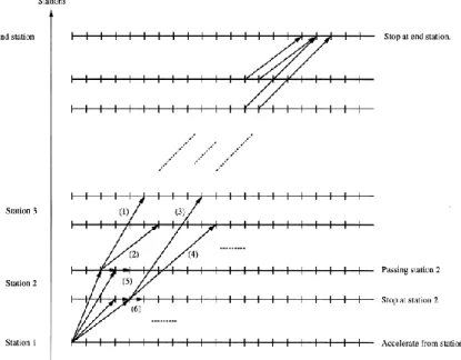
Fig. 2. Speed scenarios between train stations (Brännlund et al., 1998).

Station blocks have therefore a capacity higher or equal to 1 whereas signalling blocks have a capacity equal to 1. Fig. 1 illustrates the two types of blocks by representing a stretch of a single-track line with two station blocks with a capacity of 3 and 2 (i.e., number of parallel tracks) and three signalling blocks between the two station blocks. Note that it is possible to have more than one train between two consecutive station blocks if the safety headway blocking rules allow it. These rules will be explained later in the paper.

Fig. 2 shows that there are different speed scenarios for any train passing the blocks. The train can pass at full speed in a certain block if there is no stop before entering or after

leaving the block, as shown in scenario (1) in Fig. 2. If there is a stop before or after the block (or both), the speed is lower, as shown in scenarios (2), (3) and (4). Trains can also wait in a side track at the station block, as shown in scenario (5) to let other trains pass and in (6) for scheduled stop.

Hence, there are two different possible movement states in each end of a block:

passing at full speed (noted F) or stopping (noted S). These lead to four different speeds

scenarios depending on the state at the start and the end of the block: FF, FS, SF and SS. These different speed scenarios can be seen in Fig. 2, FF is the fastest scenario (1) and SS is the slowest (4). SF and FS are slower than FF but faster than SS. These different speeds reflect the acceleration and deceleration (i.e., braking) properties of the trains which can play an important role in determining the travel time for the different scenarios.

3.2 Model

A train request 𝑟 ∈ ℛ specifies a set of possible paths 𝒫r and assigns a utility value 𝑣𝑝 to

each of them (depending on the total travel time and the deviation from the ideal departure time). The sum of utilities 𝑣𝑝 for the selected train paths 𝑝 is the objective function in the

TTP model. The criteria, for whether a path is possible or not, are determined by the stopping stations, the departure time window and the latest arrival time. The “null path”, i.e., not scheduling or removing the requested train, is always a possible path. The set of all possible paths is denoted 𝒫 = ⋃r∈ℛ𝒫r. Note that we do not store all the possible paths

for a train request 𝑟 ∈ ℛ.

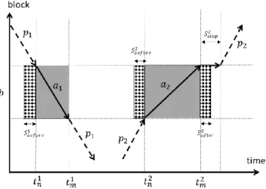
Time is discretised into time intervals 𝑡 ∈ 𝒯 and the single-track line is separated into blocks 𝑏 ∈ ℬ . The combinations (𝑡, 𝑏) make up nodes (or vertices) in a time-space directed graph. Each arc (denoted 𝑎) represents a possible train movement (i.e., FF, SF, SS or FS). For instance, train leaving block 𝑏1 at time 𝑡𝑛 accelerating from standstill,

going to block 𝑏2 at time 𝑡𝑚. This arc (denoted 𝑎1) is illustrated in the time-space graph in

Fig. 3.

Each train path 𝑝𝑟∈ 𝒫r is an ordered subset of train movements 𝑎𝑟∈ 𝒜𝑟 (set of arcs

of request r) that describes the trajectory of the train in time and space from origin to destination station. We therefore have 𝑎𝑟∈ 𝑝𝑟⊆ 𝒜𝑟 and we construct and store the

block-time graph (as shown in Fig. 2) from origin to destination for each train request. The train movement represented by an arc in the graph leads to the (not necessarily physical) occupation of a certain block-times, given by the binary matrix 𝛿𝑏𝑡𝑎 ∈ {0,1}

indicating (for a certain train movement arc 𝑎) whether the time-blocks (𝑡, 𝑏) are occupied or not. For example, arc 𝑎1(of path 𝑝1) leads to the physical occupation of block 𝑏 at

times 𝑡𝑛1, … , 𝑡𝑚−11 , i.e., 𝛿𝑏𝑡

𝑎1 _{= 1 if 𝑡}

𝑛1≤ 𝑡 ≤ 𝑡𝑚−11 (grey area in Fig. 3). The parameters 𝛿𝑏𝑡𝑎

are used in the capacity constraints of the TTP program to account for the capacity consumption of a certain train movement arc 𝑎 (part of train path 𝑝) on time-block (𝑡, 𝑏). Which paths (i.e., arcs and nodes) are possible for a specific train request is determined by the requested train departure windows, latest arrival time as well as the acceleration and deceleration (speed properties) of the train. These are provided in the input data, the speed properties are given as the travel time in each block for the different speed scenarios (i.e., FF, SF, SS or FS).

Fig. 3. Graphical representation of block occupancy. Black arrows (or arcs) show train movements,

grey areas the corresponding physical block occupancy and dotted areas the additional safety block occupancy.

To ensure a safety headway or distance between trains, several blocking rules have been adopted. For instance, if two trains are moving (as in Fig. 3), the first train (path 𝑝1)

occupies the block 𝑏 before certain minutes (𝑆𝑏𝑒𝑓𝑜𝑟𝑒1 ) of physically entering the block (at

𝑡𝑛1). Thus, the block-time occupation parameter 𝛿𝑏𝑡

𝑎1 _{for train movement 𝑎}

1 (including the

blocking rules) is 𝛿_𝑏𝑡𝑎1_{= 1 for all 𝑡 such that 𝑡}

𝑛1− 𝑆𝑏𝑒𝑓𝑜𝑟𝑒1 ≤ 𝑡 ≤ 𝑡𝑚−11 and 𝛿𝑏𝑡 𝑎1_{= 0 ,} otherwise. The same blocking rules (with 𝑆𝑏𝑒𝑓𝑜𝑟𝑒2 ) apply to the second train (path 𝑝2 in

Fig. 3). Since this train stops at the next block (for certain minutes 𝑆𝑠𝑡𝑜𝑝2 ), it can keep

occupying block 𝑏 for certain minutes (𝑆𝑎𝑓𝑡𝑒𝑟2 ) after physically leaving the block (at 𝑡𝑚2).

Thus, the parameter 𝛿_𝑏𝑡𝑎2 _{for train movement 𝑎}

2 (including the blocking rules) is 𝛿𝑏𝑡 𝑎2 _{= 1} for all 𝑡 such that 𝑡𝑛2− 𝑆𝑏𝑒𝑓𝑜𝑟𝑒2 ≤ 𝑡 ≤ 𝑡𝑚−12 + 𝑆𝑎𝑓𝑡𝑒𝑟2 and 𝛿𝑏𝑡

𝑎2 _{= 0, otherwise.}

The number of minutes 𝑆𝑏𝑒𝑓𝑜𝑟𝑒 and 𝑆𝑎𝑓𝑡𝑒𝑟 depends on the speed scenario and direction

of the meeting trains before and after the block. Fig. 3 illustrates the adopted blocking rules and the Swedish timetabling guidelines recommend using 𝑆𝑏𝑒𝑓𝑜𝑟𝑒= 𝑆𝑎𝑓𝑡𝑒𝑟= 3

minutes. (Note that we do not make any difference between headway and clearance time). These rules also guarantee that two trains in opposite directions cannot instantly swap their respective physically occupied consecutive blocks. Readers who are unfamiliar with blocking rules are invited to refer to the work by Hansen and Pachl (2014) on blocking time theory. A related work by Harrod and Schlechte (2013) compares physical and timed block occupancy.

In Fig. 3, the total capacity consumption ∑ 𝑑𝑏𝑡 𝑝 𝑝∈𝒫 = ∑ 𝛿𝑏𝑡 𝑎1 𝑎1∈𝑝1 +∑ 𝛿𝑏𝑡 𝑎2 𝑎2∈𝑝2 (for both

𝑝1 and 𝑝2 if scheduled) at block 𝑏 is 1 in the grey and dotted area and 0 elsewhere. Note

that the total capacity consumption can be greater than 1 (e.g., 2 or double occupation) if several paths (e.g., 𝑝1 and 𝑝2) occupy the same block at the same time. The constraints

(1.i) enforce that the total capacity consumption (or cumulative flow for track occupancy as in Meng and Zhou (2014) at any block 𝑏 (and any time 𝑡) is at most equal to the capacity limit 𝑐𝑏.

We summarise the notations in Table 2 for the main sets, parameters and variables in the mathematical model.

Table 2

Summary of the adopted notations.

Type Notation Description

Sets 𝒯 Time intervals {1, 2, … , 𝑡, … }

ℬ Blocks {1, 2, … , 𝑏, … }

ℛ Train requests {1, 2, … , 𝑟, … }

𝒜𝑟 Train movement arcs for request 𝑟 ∈ ℛ 𝒫𝑟 Possible train paths for request 𝑟 ∈ ℛ 𝒫 = ⋃ 𝑃𝑟

𝑟∈ℛ

All possible train paths

Parameters 𝑐𝑏 Capacity of block 𝑏 ∈ ℬ

𝑣𝑝𝑟 Utility value of train path 𝑝𝑟∈ 𝒫𝑟

𝑑_𝑏𝑡𝑝 = ∑𝛿𝑏𝑡𝑎 𝑎∈𝑝

Block occupation of time 𝑡 of block 𝑏 by train path 𝑝𝑟∈ 𝒫𝑟 Variables 𝑥𝑝∈ {0,1} Allocation state of path 𝑝 ∈ 𝒫

The TTP is now to select exactly a path 𝑝𝑟∈ 𝒫r for each train request 𝑟 ∈ ℛ such that the

total path value ∑ 𝑣𝑟 𝑝𝑟 is maximised and the timetable is feasible (capacity constraints are met). Let 𝑥𝑝∈ {0,1} be an indicator variable denoting whether path 𝑝 is selected or not.

With this, we can formulate the TTP as the mathematical program (1).

Constraints (1.i) are the capacity constraints of the blocks which do not allow the presence of more trains than the capacity limit 𝑐𝑏 in the block-time (𝑏, 𝑡). The constraints (1.ii)

specify that exactly one path is chosen for each train request. The constraints (1.iii) are the binary constraints on the path selection variable 𝑥𝑝.

Each train request 𝑟 ∈ ℛ thus has a finite set of possible paths 𝑝 ∈ 𝒫𝑟 (from the

starting station through the network to the ending station) to perform its requested duties (e.g., scheduled stops, departure window and latest arrival time). Each path is an ordered subset of movement arcs 𝑎 that describes the trajectory of the train in time-space graph.

A utility value 𝑣𝑝 can be computed for each possible path 𝑝. Summing up over all the

selected paths that are in the final timetable gives the total utility value of the train timetable, i.e., the objective value to maximise ∑𝑝∈𝒫𝑣𝑝𝑥𝑝 in program (1). In this study,

we use a basic model for the utility function which reflects the deviation penalty from an ideal departure time. Moreover, we assume that the utility values of the different trains are mutually independent which is not the case in many realistic scenarios.

The TTP is now to select one path 𝑝 ∈ 𝒫𝑟 for each train request 𝑟 ∈ ℛ, such that

capacity limits 𝑐𝑏 are not violated, and such that the total timetable utility (based on 𝑣𝑝) is

maximised. The term 𝑑_𝑏𝑡𝑝 _{(equal to ∑}

𝛿𝑏𝑡𝑎

𝑎∈𝑝 ) in constraints (1.i) corresponds to the

capacity consumption of path 𝑝 on block-time (𝑏, 𝑡) . Note that these capacity consumption parameters are also used for enforcing the blocking rules (i.e., safety occupations).

(TTP) { 𝑚𝑎𝑥 𝑥_𝑝 ∑ 𝑣𝑝𝑥𝑝 𝑝∈𝒫 s. t. { ∑ 𝑑𝑏𝑡 𝑝 𝑥𝑝 𝑝∈𝒫 ≤ 𝑐𝑏, ∀(𝑏, 𝑡) ∈ ℬ × 𝒯 (𝑖) ∑ 𝑥𝑝= 1 𝑝∈𝒫𝑟 , ∀𝑟 ∈ ℛ (𝑖𝑖) 𝑥𝑝∈ {0,1}, ∀𝑝 ∈ 𝒫 (𝑖𝑖𝑖) . (1)

The stated TTP model is an ILP with very large number of binary variables for real world instances. The combinatorial nature of the problem makes it difficult to solve for these instances using the-state-of-the-art ILP solvers. In order to get around the computational complexity of the problem, we use the classical lagrangian relaxation technique as the starting point for the solution method.

4 Solution Methods

This section focuses on deriving and describing aggregate and disaggregate solution methods for the stated TTP model. Both are based on the lagrangian relaxation and use a bundle method to solve the lagrangian dual problem.

4.1 Dual problem

In the lagrangian relaxation of (TTP), we allow the constraints (1.i) to be violated, thus allowing the presence of more trains in a time-block than the capacity limit. Moreover, this relaxation also allows the violation of the blocking rules. This violation of the capacity limit is done however at a certain price given by the lagrangian multipliers 𝜇 = {𝜇𝑏𝑡} ≥ 0. The relaxed version of (TTP) is noted (TTP)𝜇 and is formulated in problem

(2). The optimal value of the relaxed problem is noted 𝜑(𝜇).

(TTP)𝜇 { 𝜑(𝜇) ≔ max_𝑥 𝑝 ∑ 𝑣𝑝 𝑝∈𝒫 𝑥𝑝+ ∑ 𝜇𝑏𝑡(𝑐𝑏− ∑ 𝑑𝑏𝑡 𝑝 𝑝∈𝒫 𝑥𝑝 (𝑏,𝑡)∈ℬ×𝒯 ) s. t. { ∑ 𝑥𝑝= 1, ∀𝑟 ∈ ℛ 𝑝∈𝒫_𝑟 𝑥𝑝 ∈ {0,1}, ∀𝑝 ∈ 𝒫 . (2)

(TTP)𝜇 is a relaxation of (TTP) for two reasons. First, every feasible solution to (TTP) is

also a feasible solution to (TTP)𝜇. Second, the objective value of any feasible solution in

(TTP) is not greater than that in (TTP)𝜇. Hence, for each 𝜇 ≥ 0, the value of 𝜑(𝜇) in

(TTP)𝜇 is larger than or equal (i.e., an upper bound) to the optimal value of (TTP).

It is possible to further simplify the objective value of (TTP)𝜇. For a given 𝜇 ≥ 0 and

under the same constraints as in (2), 𝜑(𝜇) can be rewritten as in (3).

𝜑(𝜇) = ∑ 𝑐𝑏𝜇𝑏𝑡 (𝑏,𝑡)∈ℬ×𝒯 + max 𝑥𝑝 ∑ (𝑣𝑝− ∑ 𝜇𝑏𝑡𝑑𝑏𝑡 𝑝 (𝑏,𝑡)∈ℬ×𝒯 ) 𝑝∈𝒫 𝑥𝑝. (3)

𝑣𝑝− ∑ 𝜇𝑏𝑡𝑑𝑏𝑡 𝑝

(𝑏,𝑡)∈ℬ×𝒯 can be interpreted as a reduced utility revenue for choosing path

𝑝 ∈ 𝒫 (i.e., 𝑥𝑝= 1) given the multipliers 𝜇 . This means that (TTP)𝜇 is equivalent to

finding the shortest path in the time-space graph for each train request. Shortest in the sense that the path yields the maximum reduced utility revenue where the multipliers represent the cost of traversing the arcs in that path. Shortest path problems have well-established solution algorithms and are relatively easy to solve. In this model, we developed a shortest path algorithm based on topological sorting. This is justified by the fact that the time-space graph is a weighted directed acyclic graph (Cormen et al., 2009).

As just noted, 𝜑(μ) is an upper bound to the optimal value of (TTP). Thus, the dual problem (D) is to find the optimal solution μ∗ _{that gives the smallest bound as in (4).}

Since there are only a finite number of shortest path combinations, 𝜑 is piecewise linear. It is therefore a convex function since it is the maximum of a set of linear functions. Moreover, 𝜑 has a lower bound, i.e., any feasible solution to the original problem (TTP). Therefore, (D) has a global minimum 𝜑∗ _{at the optimal multipliers 𝜇}∗_.

(D) {𝜇∗: = argmin 𝜑(𝜇)

s. t. 𝜇 ≥ 0 . (4)

Let us assume that for an arbitrary value 𝜇̅ ≥ 0, the maximum in (TTP)𝜇̅ is achieved at

𝑥̃(𝜇̅) = (𝑥̃𝑝)𝑝∈ 𝒫. Inserting the corresponding 𝑥̃(𝜇̅) in the objective of (TTP)𝜇 gives a

linear (in 𝜇) function 𝜑̃(𝜇) = ∑𝑝∈𝒫𝑣𝑝𝑥̃𝑝+ ∑ 𝜇𝑏𝑡(𝑐𝑏− ∑ 𝑑𝑏𝑡 𝑝 𝑝∈𝒫 𝑥̃𝑝

𝑏𝑡 ), that is equal to

𝜑(𝜇) at 𝜇̅. This linear function corresponds to a supporting plane to the graph of 𝜑. The slope of this function is given by the matrix 𝑔(𝜇̅) = (𝑔̅𝑏𝑡) ≔ (𝑐𝑏− ∑ 𝑑𝑏𝑡

𝑝

𝑝∈𝒫 𝑥̃𝑝) which is

a subgradient of 𝜑 at 𝜇̅. Thus, the supporting linear function to 𝜑 at 𝜇̅ can be written as in equation (5) where * denotes the inner product between two matrices (i.e., component wise).

𝜑(𝜇̅) + 𝑔(𝜇̅) ∗ (𝜇 − 𝜇̅). (5)

In order to solve (D), we use the (aggregate) bundle method by Kiwiel (1990), described in the next section. Based on this method, the subsequent section derives the disaggregate approach to solve (D) for the train timetabling problem TTP.

4.2 Aggregate bundle method

For 𝜇 = 𝜇̅, the (possibly many) 𝑥̃(𝜇̅), i.e., maximum in (TTP)𝜇, give the subgradients to

𝜑 at 𝜇̅. Suppose that we currently are at 𝜇 = 𝜇𝑘, and that we have chosen to approximate

𝜑 by the supporting planes computed in iterations 𝑙 ∈ ℒ𝑘, where ℒ𝑘 is the bundle of active

supporting planes of 𝜑 at iteration 𝑘. Let the corresponding subgradients be {𝑔𝑙}𝑙∈ℒ𝑘. Then in the standard aggregate bundle method, we compute a new tentative solution as the solution to the subproblem formulated in (6) where |∙| denotes the Euclidean norm (2-norm) of a matrix reshaped into a vector, and 𝜑̅𝑘_{(𝜇) ∶= max}

𝑙∈ℒ𝑘{𝜑(𝜇𝑙) + 𝑔𝑙∗ (𝜇 − 𝜇𝑙)} is the maximum of the supporting linear functions at 𝜇𝑙, for 𝑙 ∈ ℒ𝑘, giving an outer

linearization of 𝜑. The quadratic second term helps to avoid taking large steps and the step size is adjusted using the control parameter 𝑢𝑘 at each iteration.

(D̅_𝑘agg ) {min 𝜑̅ 𝑘_{(𝜇) +}𝑢𝑘 2 |𝜇 − 𝜇𝑘| 2 s. t. 𝜇 ≥ 0, . (6)

In order to get around the inner maximisation, (D̅

𝑘 agg

) can be formulated as a single minimisation problem by adding an additional variable as well as new constraints for the supporting linear functions. This leads to the equivalent problem (7).

(D̅_𝑘agg) { min 𝑣,𝜇 𝑣 + 𝑢𝑘 2 |𝜇 − 𝜇𝑘| 2 s. t. {𝑣 ≥ 𝜑(𝜇𝑙) + 𝑔𝑙∗ (𝜇 − 𝜇𝑙), ∀𝑙 ∈ ℒ𝑘 (𝑖) 𝜇 ≥ 0 (𝑖𝑖) . (7)

The matrices 𝜇𝑙 for 𝑙 ∈ ℒ𝑘 can be extremely large and lead to an excessive memory usage.

Therefore, we suggest an equivalent formulation of the supporting linear functions in which scalars, 𝛹𝑘𝑙≔ 𝜑(𝜇𝑙) + 𝑔𝑙∗ (𝜇𝑘− 𝜇𝑙) at k and for all 𝑙 ∈ ℒ𝑘, are stored instead of

the matrices. The right-hand side of the constraint (7.i) can now be rewritten according to equation (8).

𝜑(𝜇𝑙) + 𝑔𝑙∗ (𝜇 − 𝜇𝑘) + 𝑔𝑙∗ (𝜇𝑘− 𝜇𝑙) = 𝛹𝑘𝑙+ 𝑔𝑙∗ (𝜇 − 𝜇𝑘). (8)

Hence, problem (7) (or equivalently (6)) can be reformulated as in (9).

(D̅_𝑘agg ) { min 𝑣,𝜇 𝑣 + 𝑢𝑘 2 |𝜇 − 𝜇𝑘| 2 s. t. {𝑣 ≥ 𝛹𝑘𝑙+ 𝑔𝑙∗ (𝜇 − 𝜇𝑘), ∀𝑙 ∈ ℒ𝑘 (𝑖) 𝜇 ≥ 0 (𝑖𝑖) . (9)

The advantage of the formulation in (9) is that it allows to save in the memory usage. Instead of storing the bundle of matrices 𝜇𝑙, as in (7), we only store the scalars 𝛹𝑘𝑙 and use

the matrix of multipliers 𝜇𝑘 at the current iteration 𝑘. Moreover, 𝛹𝑘𝑙 can be updated

recursively, without the need for retrieving the matrices 𝜇𝑙, whenever the multipliers are

updated (i.e., 𝜇𝑘+1≠ 𝜇𝑘) as

𝛹𝑘+1,𝑙 = 𝛹𝑘𝑙+ 𝑔𝑙∗ (𝜇𝑘+1− 𝜇𝑘) , (10)

so that the supporting linear functions always have the current 𝜇𝑘 as “foot point”.

Let 𝑦𝑘+1 be the optimal solution to (D̅𝑘 agg

). At 𝑦𝑘+1 we evaluate the dual objective 𝜑

by solving (TTP)𝜇 for 𝜇 = 𝑦𝑘+1. We might then get a new supporting plane, including a

new subgradient 𝑔𝑘+1. We define the achieved descent as 𝜑̅𝑘(μ𝑘) − 𝜑(y𝑘+1) and the

forecasted one as 𝜑̅𝑘_(μ

𝑘) − 𝜑̅𝑘(y𝑘+1). If the ratio of the achieved descent by the

forecasted one is larger than a certain step quality threshold 𝑚𝐿∈ [0,1] (e.g., 10 %) then

we set 𝜇𝑘+1= 𝑦𝑘+1, and the new ℒ𝑘+1 will incorporate the active supporting planes from

ℒ𝑘 as well as the newly generated supporting plane. If otherwise the ratio is not large

enough, we set 𝜇𝑘+1= 𝜇𝑘 and ℒ𝑘+1 will only add the newly generated supporting plane to

ℒ𝑘. Thus, the polyhedral approximation of 𝜑 is always improved at each iteration.

The step control parameter 𝑢𝑘+1 is adjusted in both cases (i.e., ratio is large enough or

not). It is set so that the curvature of the objective in (D̅

𝑘 agg

of 𝜑. We use the same step control update strategy as the one adopted by Kiwiel (1995).

4.3 Disaggregate bundle method

In the disaggregated bundle method, the main idea is to linearly approximate (with supporting planes) the function 𝜑 for each train request 𝑟 ∈ ℛ instead of the approximation of the aggregated sum of all the requests. Thus, we extract more information from the solutions to the subproblems (TTP)𝜇 by considering a disaggregate

function for each train request that we note 𝜑𝑟 for all 𝑟 ∈ ℛ.

𝜑(𝜇) = ∑ 𝜑𝑟(𝜇) 𝑟∈ℛ

+ ∑ 𝑐𝑏𝜇𝑏𝑡 (𝑏,𝑡)∈ℬ×𝒯

. ₍₁₁₎

The formulation in (11) shows how the dual objective function is separated into request-dependent functions 𝜑𝑟 which are defined in program (12) as a maximisation problem for

a given value of the multipliers 𝜇. These 𝜇𝑏𝑡 can be interpreted as prices for using the

block 𝑏 at time 𝑡, an interpretation that we will return to in the concluding section.

𝜑𝑟(𝜇) ≔ max 𝑥𝑝 ∑ (𝑣𝑝− 𝑝∈𝒫_𝑟 ∑ 𝜇𝑏𝑡𝑑𝑏𝑡 𝑝 (𝑏,𝑡)∈ℬ×𝒯 )𝑥𝑝 s. t. { ∑ 𝑥𝑝= 1 (𝑖) 𝑝∈𝒫𝑟 𝑥𝑝∈ {0,1}, ∀𝑝 ∈ 𝒫𝑟 (𝑖𝑖) . (12)

The disaggregate dual problem (13), noted (Ddis_{), will be slightly different from (D) that}

is used in the aggregate approach.

(Ddis_{) {}min𝜇 ∑ 𝜑𝑟(𝜇) + ∑ 𝜇𝑏𝑡 (𝑏,𝑡)∈ℬ×𝒯 𝑐𝑏 𝑟∈ℛ s. t. 𝜇 ≥ 0 . (13)

At iteration k in the disaggregate approach, each objective component 𝜑𝑟 has its own

bundle ℒ𝑘𝑟, with the subgradients defined as 𝑔𝑟𝑙: = −𝑑𝑝̂𝑟𝑙 , where 𝑝̂𝑟𝑙∈ 𝒫𝑟 is the shortest

path in the sense that it leads to the maximal revenue for 𝜇 = 𝜇𝑙 in (TTP)𝜇.

As with the aggregate approach, we use the subgradients to build supporting linear functions that are used as an outer approximation. In the disaggregate approach the outer approximation is computed for each objective component 𝜑𝑟. Thus, the disaggregate

bundle method problem is written as follows

(D̅_𝑘dis₎ { min ∑ 𝑣𝑟 𝑟∈ℛ + ∑ 𝑐𝑏𝜇𝑏𝑡 (𝑏,𝑡)∈ℬ×𝒯 +𝑢𝑘 2 |𝜇 − 𝜇𝑘| 2 s. t. {𝑣𝑟≥ 𝜑𝑟(𝜇𝑙) + 𝑔𝑟𝑙∗ (𝜇 − 𝜇𝑙), ∀𝑙 ∈ ℒ𝑘 𝑟 _{∀𝑟 ∈ ℛ (𝑖)} 𝜇 ≥ 0 (𝑖𝑖) . (14)

approach in equation (8), instead of storing all the previous matrices of multipliers 𝜇𝑙, we

only store the corresponding scalar parameters 𝛹𝑘𝑙𝑟 that we define similarly as follows

𝛹𝑘𝑙𝑟 ∶= 𝜑𝑟(𝜇𝑙) + 𝑔𝑟𝑙∗ (𝜇𝑘− 𝜇𝑙). (15)

The parameters are updated in a similar way to the aggregate case that is previously described in (10). Thus, the formulation of (D̅_𝑘dis_{) can be rewritten using the scalar}

parameters. So, at iteration k, we have

(D̅𝑘dis) { min ∑ 𝑣𝑟+ ∑ 𝑐𝑏𝜇𝑏𝑡 (𝑏,𝑡)∈ℬ×𝒯 +𝑢𝑘 2 |μ − μ𝑘| 2 𝑟∈ℛ s. t. {𝑣𝑟≥ 𝛹𝑘𝑙 𝑟 _{+ 𝑔} 𝑟𝑙∗ (𝜇 − 𝜇𝑘), ∀ 𝑙 ∈ ℒ𝑘𝑟 , ∀𝑟 ∈ ℛ (𝑖). 𝜇 ≥ 0 (𝑖𝑖) (16)

Note that formulation (16), unlike (9), includes the term ∑(𝑏,𝑡)∈ℬ×𝒯𝑐𝑏𝜇𝑏𝑡 since this term is

shared between the different train requests 𝑟 ∈ ℛ and is therefore not separable.

We can further simplify (16) by introducing 𝑠 = 𝜇 − 𝜇𝑘 to get the following

formulation (D̅_kdis₎ { min ∑ 𝑣𝑟+ ∑ (𝜇𝑏𝑡𝑘 + 𝑠𝑏𝑡) (𝑏,𝑡)∈ℬ×𝒯 𝑐𝑏+ 𝑢𝑘 2 |𝑠| 2 𝑟∈ℛ s. t. {𝑣𝑟≥ 𝛹𝑘𝑙 𝑟 _{+ 𝑔} 𝑟𝑙∗ 𝑠, ∀ 𝑙 ∈ ℒ𝑘𝑟 , ∀𝑟 ∈ ℛ (𝑖) 𝑠 ≥ −𝜇𝑘 (𝑖𝑖) . (17)

In theory, the disaggregate bundle formulation improves the aggregate one in that it allows to make a more accurate linear approximation of the dual objective function 𝜑 by taking advantage of the individual train requests (𝛹𝑘𝑙𝑟 in contrast with 𝛹𝑘𝑙). This allows to

extract and use more dual information per iteration from the shortest path results. Another advantage is that the disaggregate formulation can be implemented as a parallel program for each train request to improve the computational time (Gurdan and Kaeslin, 2015).

5 Experimental Setup and Results

This section provides details about the case study. We first give implementation-related information before presenting the input data and the experiment scenarios. Finally, the results are presented and discussed before discussing further notes.

5.1 Implementation

Both solution methods, i.e., the aggregate and the disaggregate bundle method, are developed in MATLAB. The methods call a C++ function that computes the shortest path given the prices 𝜇 = {𝜇𝑏𝑡} of occupying the block-times. The information between the

two programming environments is exchanged using mex functions which are subroutines that allow MATLAB programs to call C++ functions which have faster access to memory (MathWorks, 2016). Fig. 4 gives an overview of the software architecture that was implemented.

Fig. 4. Software architecture of the model implementation.

In order to speed up the computation of the shortest path algorithm, the path networks (the graph of possible train movements in time-space) are constructed once and are stored in the C++ environment memory for use in all the iterations of the bundle method. Dijkstra algorithm is used for the shortest path computation (Dijkstra, 1959). The MATLAB program (i.e., bundle method) calls at first a C++ function that allocates memory and constructs the path networks from the input data before performing the bundle iteration which is implemented using interior point method.

5.2 Input data

The input data that is used to test the two algorithms is based on train operations on the Iron Ore line (Malmbanan) in northern Sweden. The stretch that is considered is between

Kiruna (Sweden) and Narvik (Norway) as in Fig. 5.

The input data was provided by the Swedish National Transport Administration (Trafikverket). It consists of the following:

• Signalling blocks (with waiting stations) on the line

• Travel time to traverse the associated block for different speed scenarios (SF, SS, FS, FF)

• Number of tracks (i.e., capacity) of each waiting station

In this study we consider, for the sake of simplicity, only one type of trains having the same speed properties for the different requested train paths. This means that all the trains have similar travel times between blocks on the line.

We consider 32 train requests during a weekday with 6 (SJ AB) passenger trains and 26 freight trains, operated by the freight operators (e.g., LKAB, Green Cargo and Hector Rai). Each request includes the following information:

• Departure and arrival stations • Ideal departure time

Fig. 5. The Iron Ore line between Narvik (in Norway) and Kiruna (in Sweden).

Each train request specifies an ideal departure time. We consider in this study that trains have a departure windows around this ideal departure time of around 30 minutes, i.e., trains are can depart up to 30 minutes before and up to 30 minutes after the ideal departure time.

The value of a path is the (weighted) sum of the deviation from ideal departure time (as in Fig. 6) and the path’s total running time from departure to arrival station. We distinguish between freight and passenger services in the peak (𝑣𝑚𝑎𝑥 in Fig. 6) of the

deviation function. In this experiment, we set it to 500 for all the 26 freight trains and to 1000 for the remaining 6 passenger trains in order to reflect the assumption that the departure time for passenger trains is generally more valuable. The choice of values for train requests getting fulfilled at all, i.e., its value compared to the null path, has been arbitrarily set at different levels for freight (500) and passenger (1000) services. It has been suggested that this input to the optimisation exercise emanates from an explicit bidding process (on-track competition) where different (competing) operators define the paths they request and the value function of being allocated a path. The utility value 𝑣𝑝

associated with the allocated path p ∈ 𝒫r then specifies the operator’s benefit of being

able to run each service. Solving the track allocation problem more generally comprises two components; the optimisation problem which is addressed by the present paper; and the valuation problem which can be handled by operators submitting bids for each path. The latter problem is out of the scope of this paper but was addressed by Nilsson (2002).

Moreover, we consider that each (passenger) train has a minimal compulsory waiting time of 2 min at every scheduled waiting. We also consider the blocking rules to ensure a certain safety distance between trains.

In order to check the models on different problem instances, we constructed three different test cases from the given data. Table 3 lists the different experiment scenarios and their characteristics.

Table 3

Test cases and their characteristics.

Test case Terminal stations # of stations # of blocks

S1 Bjørnfjell - Narvik 5 14

S2 Kiruna – Torneträsk 7 23

S3 Kiruna – Vassijaure 14 51

The test case scenarios correspond to an increasingly longer stretch of the Iron Ore line, i.e., increasing number of stations and blocks. The 32 requested train paths are as previously described and are adjusted to run between the terminal station of the considered line stretch of each scenario.

5.3 Results

The experimental tests were executed on a remote computer with two processors Intel(R) Xeon(R) CPU E5645. Each processor has a clock frequency of 2.40 GHz and 12 MB cache memory; the RAM memory is 80 GB.

The models have several parameters and initialisations to be set before starting the execution. The parameter values are given in Table 4.

Table 4

Algorithm parameters and their values

Parameter Value

Time discretisation step 30 seconds

Step quality threshold 𝑚𝐿= 0.1 (= 10%)

Initial step control value 𝑢0= 1

Minimal step control 𝑢𝑚𝑖𝑛= 10−10

Maximal number of iterations 𝑘𝑚𝑎𝑥= 200 Initial prices (multipliers) 𝜇0= 0 Tolerance (stopping condition) 𝜖 = 10−13

Both models were tested under the same conditions, i.e., same machine, parameters and input data. Fig. 7 shows the comparison between the dual objectives in the aggregated and disaggregate approaches for the test cases S1 – S3.

In the three test cases, the optimisation of the dual objective function has a similar behaviour for the two approaches in the first iterations. However, after a certain number of iterations, the minimisation in the disaggregate approach becomes faster as more information is collected in the iteration bundle. This leads to a faster convergence using the disaggregate approach.

Fig. 7. Dual objective for the two approaches in the test cases S1 to S3 (from top). Table 5

Initialisation and execution time in the test cases S1 – S3 Case Initialisation time

(in min) Execution time – aggregate (in min) Execution time – disaggregate (in min) Execution time improvement S1 26.44 40.36 24.11 40.3% S2 39.17 49.71 27.13 45.4% S3 213.19 (≈ 3.5h) 209.09 (≈ 3.5h) 169.72 (≈ 2.8h) 18.8% * The improvement is relative to the aggregate approach.

Table 5 presents the computation times for the initialisation and execution time of the test cases. The initialisation time (column 2) is the time needed to read data and construct the train movement graph (see Fig. 4). This step is similar for both variants and is performed

only once for each test case. The execution times (columns 3 and 4) relate to the time to execute the bundle method (with iterative calls to the shortest path algorithm). Both variants call the same algorithm for computing the shortest path on the same train movement graph, so the improvement in execution time is mainly due to the fewer number of iterations performed by the disaggregate variant (see Fig. 7). Moreover, if the solution algorithm stops after reaching a maximum number of iterations (e.g., 𝑘𝑚𝑎𝑥 ≥ 7

for Fig. 7), the disaggregate solution is generally more accurate, i.e., better dual objective value, which is mainly due to the faster convergence of the approach after a number of iterations.

Note that the computation times in Table 5 increase substantially for S3 (larger instance). Moreover, the savings in the execution times, when using disaggregation, decrease. Therefore, disaggregation may give limited savings when used to solve larger instances of the problem, but more tests are needed to reveal this variant’s convergence properties.

Testing the two approaches also provides additional useful information. For instance, the solution to the dual problem provides values for the multipliers 𝜇𝑏𝑡 which can be used

for pricing the infrastructure capacity in time-space. Fig. 8(a) presents the resulting optimal infrastructure pricing (or multipliers) for test case S1 using the disaggregate approach. The vertical axis refers to the blocks and the horizontal one to the time steps (30 seconds for each timestep), higher prices are shown in black. The corresponding optimal (not necessarily feasible) dual solution timetable (i.e., selected train path for each request) can be visualised in the graphical (time-space) timetable in Fig. 8(b) where colours are used to differentiate between the train requests. Each selected train path is shown in a different colour. Since this is the optimal solution of the relaxed TTP, plotting all the selected train paths at the final iteration of the algorithm will not necessarily lead to a feasible timetable. Such a timetable can be obtained from the relaxed solution (together with all the generated train paths) as explained in section 5.4.

(a) Optimal mulipliers (or capacity prices) for each block and time, higher values in black.

(b) Selected train paths at optimal dual solution, colours to distinguish between train paths.

Similar figures can be produced for the aggregate case. However, the disaggregate approach yields higher multiplier values (prices), train paths with more stops and more generated train path alternatives. The results in Fig. 8 indicate that having train path requests with close (or similar) ideal departure times (i.e., competition for the slot) yields higher pricing of capacity around the block-times with most conflicts, e.g., mainly around the departure stations and ideal departure times. If these conflicting train paths are requested by different concurrent operators (e.g., open access), such prices can be used to sell departure slots or as congestion fees in the access charges.

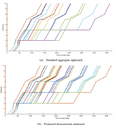
In each iteration, the shortest path algorithm is called to find the best paths for a given pricing. This leads to an additional output of the algorithm, i.e., a set of generated (possible) train paths for each request. Therefore, each request has a set of alternative paths which contains “the” optimal path (including the null path, i.e., cancelling the train) that will be selected in the final optimal (feasible) timetable.

(a) Standard aggregate approach.

(b) Proposed disaggregate approach.

Fig. 9. Generated train path alternatives for the first request in test case S1, colours to distinguish

Fig. 9 illustrates an example of a set of generated paths for the first train request in test case S1. The first graph (a) shows the aggregate approach and the second one (b) the disaggregate approach. The disaggregate approach generates a larger set of paths compared to the aggregate one, e.g., 24 paths instead of 14 as in

Fig. 9. The null path is always part of such a set to allow cancel train requested train (i.e., vertical line in the origin). The distribution of the generated paths is affected by several parameters, e.g., the optimisation approach (aggregate or disaggregate), the utility value of the objective function (freight or passenger) and other conflicting train requests.

The generated set of paths from the disaggregate methods has therefore more potentially optimal train paths per request that can be selected in the final feasible timetable. This larger set of generated paths is particularly important in finding better quality feasible solutions. Branch-and-bound is a technique that can be used to find such a solution based on the resulting optimal solution of the relaxation problem.

In practice, both variants can be used to solve small to medium size instance of the problem. In particular, train timetabling instances with highly congested traffic (i.e., several conflicting train requests and/or limited railway capacity). The case study has shown that disaggregation allows savings in computation time. Moreover, the construction of the train movement graph is done once and can be performed ahead of executing the bundle solution methods which can allow substantial savings in the total solution time. Another advantage, specific to the disaggregate method, is the potential of a parallel implementation which would lead to further savings in computation times. However, even with the advantages of the disaggregate variant (including the parallelisation), the method seems to be unsuitable for real time rescheduling, especially for larger instances. Moreover, the formulation of the objective function assumes that each train request has a certain utility function which is not always available and may be difficult to estimate. Alternative recent approaches exist such as auction (Pena-Alcaraz, 2015) or societal costs (Ait-Ali et al., 2020).

5.4 Fractional solution and final feasible timetable

The relaxed fractional solution from the solution methods will not necessarily lead to a feasible timetable, as in Fig. 8(b), unless the studied instance correspond to an unimodular constraint matrix, the TTP is solved in this case.

However, the relaxed optimal solution often yields fractional values for the integer variables. In this case, the multipliers and the generated train paths combined with a branch-and-bound method can be used to find a good quality feasible timetable. A unique path (including “null-path”) is selected for each request from the generated train paths to form the feasible timetable.

In order to compute the fractional solution (i.e., 𝑥 = (𝑥𝑝) not necessarily integer) of

the relaxed (TTP), we use the dual solution of the dual disaggregate problem (Ddis_{). For}

this, we note 𝜆 = (𝜆𝑟𝑙) as the dual solution of (D̅𝐾dis) in (14) at the last iteration K of the

iterative disaggregate bundle algorithm. The dual multipliers 𝜆𝑟𝑙 are associated with the

problem constraint for request 𝑟 ∈ ℛ and bundle iteration 𝑙 ∈ ℒ𝐾𝑟. The fractional solution

for a path 𝑝𝑟∈ 𝒫𝑟 is formulated in (18) where 𝑆𝑃𝑙𝑟 denotes the shortest path for request 𝑟

at iteration 𝑙 in the iterative disaggregate bundle algorithm.

𝑥𝑝𝑟= ∑ 𝜆𝑟𝑙

𝑙∈ℒ_𝐾r 𝑝𝑟=𝑆𝑃𝑙𝑟

≥ 0 .

(18)

It can be shown that the dual solution satisfies ∑ 𝑙∈ℒ_𝐾𝑟𝜆𝑟𝑙 = 1 at the optimum. Thus, the

fractional solution is 𝑥𝑝_𝑟∈ [0,1] , ∀𝑝𝑟∈ 𝒫𝑟, ∀𝑟 ∈ ℛ and can be interpreted as the

likelihood of choosing path 𝑝𝑟 for request 𝑟 in the final feasible timetable. For instance, if

a certain path 𝑝𝑟 is the shortest path during all the 𝐾 iterations of the algorithm (∀𝑙 ∈ ℒ𝐾𝑟),

we have 𝑥𝑝𝑟= ∑ 𝑙∈ℒ𝐾𝑟 𝜆𝑟𝑙

𝑝𝑟=𝑆𝑃𝑙𝑟

=∑ 𝑙∈ℒ_𝐾𝑟𝜆𝑟𝑙 = 1 and hence this path (i.e., 𝑝𝑟) is chosen in the

final feasible timetable.

Adapted variants of branch-and-bound methods, e.g., rapid branching (Borndörfer et al., 2013), can be used to find an optimal feasible combination of the generated paths using their respective fractional solution value from the disaggregate approach.

6 Conclusions

Finding a faster solution to the train timetabling problem is useful for many situations in applied railway planning, both for long-term and short-term planning, and when trying to construct capacity allocation processes with several stakeholders. This paper contributes to this by presenting an improved, parallelisable and easily implementable bundle method that can be used when solving the dual problem arising from the relaxation of a train timetabling problem. Compared to the standard bundle method, the new method uses disaggregate information and yields more accurate solutions faster. When solving the problem, lagrangian multipliers are obtained for each train request that can be interpreted as the price incurred by the network for using the train path. This is useful as it can give insights to the infrastructure manager on different aspects such as track access charges or lack of capacity.

Numerical results suggest that the new, disaggregate method tends to give shorter execution times and better accuracy, compared to the standard, aggregate bundle method. Moreover, the disaggregate method generates larger sets of possible train paths, which is a useful feature for branch-and-bound algorithms. The disaggregate approach has therefore the potential to improve lagrangian-based solution methods for discrete time and space formulations of TTPs. Possible future works include investigating the scalability of this new approach with further tests and analysis using other case studies. The proposed disaggregation approach can also be used with solution methods (other than bundle methods) and compare its performances with the corresponding standard variant.

Conflicts of Interest

The authors declare that this research has no conflicts of interest.

Acknowledgment

This research is part of the project Socio-economically efficient allocation of railway capacity, SamEff (Samhällsekonomiskt effektiv tilldelning av kapacitet på järnvägar) which is funded by a grant from the Swedish Transport Administration (Trafikverket). The

authors are grateful to Martin Aronsson, Tobias Gurdan and Alain Kaeslin for the valuable discussions and comments as well as to three anonymous reviewers and journal editors for helpful suggestions.

References

AIT-ALI, A., WARG, J. & ELIASSON, J. 2020. Pricing commercial train path requests based on societal costs. Transportation Research Part A: Policy and Practice, 132, 452-464.

BACH, L., MANNINO, C. & SARTOR, G. MILP approaches to practical real-time train scheduling: the Iron Ore Line case. International Network Optimization Conference (INOC), 2018.

BORNDÖRFER, R., LÖBEL, A., REUTHER, M., SCHLECHTE, T. & WEIDER, S. 2013. Rapid branching. Public Transport, 5, 3-23.

BRÄNNLUND, U., LINDBERG, P. O., NÕU, A. & NILSSON, J.-E. 1998. Railway Timetabling using Lagrangian Relaxation. Transportation Science, 32, 358-369. CACCHIANI, V., CAPRARA, A. & TOTH, P. 2008. A column generation approach to

train timetabling on a corridor. 4OR, 6, 125-142.

CAPRARA, A., FISCHETTI, M. & TOTH, P. 2002. Modeling and solving the train timetabling problem. Operations Research, 50, 851-861.

CAPRARA, A., MONACI, M., TOTH, P. & GUIDA, P. L. 2006. A Lagrangian heuristic algorithm for a real-world train timetabling problem. Discrete Applied

Mathematics, 154, 738-753.

CORMEN, T. H., LEISERSON, C. E. & RIVEST, R. L. 2009. Introduction to

Algorithms, Cambridge, US, The MIT Press.

DIJKSTRA, E. W. 1959. A note on two problems in connexion with graphs. Numerische

mathematik, 1, 269-271.

FORSGREN, M., ARONSSON, M. & GESTRELIUS, S. 2013. Maintaining tracks and traffic flow at the same time. Journal of Rail Transport Planning &

Management, 3, 111-123.

GURDAN, T. & KAESLIN, A. 2015. Parrallelised Shortest Path Algorithm for Railway

Timetable Construction. MA Master thesis, KTH.

HANSEN, I. A. & PACHL, J. 2014. Railway timetabling & operations. Eurailpress,

Hamburg.

HARROD, S. & SCHLECHTE, T. 2013. A direct comparison of physical block occupancy versus timed block occupancy in train timetabling formulations.

Transportation Research Part E: Logistics and Transportation Review, 54,

50-66.

HARROD, S. S. 2012. A tutorial on fundamental model structures for railway timetable optimization. Surveys in Operations Research and Management Science, 17, 85-96.

JAMILI, A., SHAFIA, M. A., SADJADI, S. J. & TAVAKKOLI-MOGHADDAM, R. 2012. Solving a periodic single-track train timetabling problem by an efficient hybrid algorithm. Engineering Applications of Artificial Intelligence, 25, 793-800.

KIWIEL, K. C. 1990. Proximity control in bundle methods for convex nondifferentiable minimization. Mathematical Programming, 46, 105-122.

KIWIEL, K. C. 1995. Approximations in proximal bundle methods and decomposition of convex programs. Journal of Optimization Theory and Application, 84, 529-548.

LUSBY, R. M., LARSEN, J., EHRGOTT, M. & RYAN, D. 2011. Railway track allocation: models and methods. OR Spectrum, 33, 843-883.

MATHWORKS. 2016. Introducing MEX Files [Online]. source MEX fileC, C++, or

Fortran source code file. Available:

http://se.mathworks.com/help/matlab/matlab_external/introducing-mex-files.html [Accessed October 2015].

MENG, L. & ZHOU, X. 2014. Simultaneous train rerouting and rescheduling on an N-track network: A model reformulation with network-based cumulative flow variables. Transportation Research Part B: Methodological, 67, 208-234. NILSSON, J.-E. 2002. Towards a welfare enhancing process to manage railway

infrastructure access. Transportation Research Part A, 36, 419–436.

PENA-ALCARAZ, M. M. T. 2015. Analysis of Capacity Pricing and Allocation

Mechanisms in Shared Railway Systems. PhD, MIT - Massachusetts Institute of

Technology.

QUAGLIETTA, E., PELLEGRINI, P., GOVERDE, R. M. P., ALBRECHT, T., JAEKEL, B., MARLIÈRE, G., RODRIGUEZ, J., DOLLEVOET, T., AMBROGIO, B., CARCASOLE, D., GIAROLI, M. & NICHOLSON, G. 2016. The ON-TIME real-time railway traffic management framework: A proof-of-concept using a scalable standardised data communication architecture. Transportation Research

Part C: Emerging Technologies, 63, 23-50.

TÖRNQUIST, J. 2012. Design of an effective algorithm for fast response to the re-scheduling of railway traffic during disturbances. Transportation Research Part

C: Emerging Technologies, 20, 62-78.

TÖRNQUIST, J. 2015. Computational decision-support for railway traffic management and associated configuration challenges: An experimental study. Journal of Rail

Transport Planning & Management, 5, 95-109.

TÖRNQUIST, J. & PERSSON, J. A. 2007. N-tracked railway traffic re-scheduling during disturbances. Transportation Research Part B: Methodological, 41, 342-362. XU, X., LI, K., YANG, L. & YE, J. 2014. Balanced train timetabling on a single-line

railway with optimized velocity. Applied Mathematical Modelling, 38, 894-909. YUE, Y., WANG, S., ZHOU, L., TONG, L. & SAAT, M. R. 2016. Optimizing train

stopping patterns and schedules for high-speed passenger rail corridors.

Transportation Research Part C: Emerging Technologies, 63, 126-146.

ZHANG, Y., D'ARIANO, A., HE, B. & PENG, Q. 2019a. Microscopic optimization model and algorithm for integrating train timetabling and track maintenance task scheduling. Transportation Research Part B: Methodological, 127, 237-278. ZHANG, Y., PENG, Q., YAO, Y., ZHANG, X. & ZHOU, X. 2019b. Solving cyclic train

timetabling problem through model reformulation: Extended time-space network construct and Alternating Direction Method of Multipliers methods.