Regional Productivity and Import Accessibility : Investigating the effect of imported goods on labour productivity levels at the municipal level

(1)

J

Ö N K Ö P I N G

I

N T E R N A T I O N A L

B

U S I N E S S

S

C H O O L JÖNKÖPING UNIVERSITY

R e g i o n a l P r o d u c t i v i t y a n d

I m p o r t A c c e s s i b i l i t y

I n v e s t i g a t i n g t h e e f f e c t o f i m p o r t e d g o o d s o n l a b o u r

p r o d u c t i v i t y l e v e l s a t t h e m u n i c i p a l l e v e l

Master Thesis within Economics

Author: Anton Lindbom

Tutors: Professor Charlie Karlsson PhD Candidate Lina Bjerke

(2)

i

Dedication

I dedicate this master thesis to the memory of my mother Åsa Curtsdotter who passed away last year. You always encouraged me to do my best and inspired me to be a good and kind man. I miss you and I love you.

Stockholm, Sweden, March 2009 Anton Lindbom

(3)

ii Master Thesis in Economics Title: Regional Productivity and Import Accessibility: A Study of Regional Growth Author: Anton Lindbom Tutors: Professor Charlie Karlsson and PhD Candidate Lina Bjerke Date: March 2009 Subject: Imports, Productivity, Accessibility, Regional Growth

Abstract

The purpose of this thesis is to estimate if imports of goods at the municipal level have an effect on labour productivity. The theoretical framework used in the thesis is based on the concept of accessibility, city growth in connection to imports, networks and nodes, clusters and economies of scale. Seven independent variables were chosen for the regression, three import accessibility variables to estimate if there is a connection between imports and productivity and Technology Gap, Population Density, Distance to Stockholm and Time. The regression model itself is built on the regression model in Fingleton (2001) but reformulated in this master thesis. Due to high collinearity between the accessibility variables they were added together to measure total accessibility. Regression results showed significant t‐statistics for all variables included confirming that there is a relationship between imports of goods and labour productivity.

(4)

iii Magisteruppsats inom Nationalekonomi Titel: Regional Produktivitet och Importillgänglighet: En Studie i Regional Tillväxt Författare: Anton Lindbom Handledare: Professor Charlie Karlsson och Doktorand Lina Bjerke Datum: Mars 2009 Ämnesord: Import, Produktivitet, Tillgänglighet, Regional Tillväxt

Sammanfattning

Syftet i denna magisteruppsats är att analysera om import av produkter på kommunal nivå är korrelerad med kommunal arbetsproduktivitet. Det teoretiska kapitlet är baserat på konceptet tillgänglighet, tillväxt och import i stadsregioner, nätverk och noder samt skalekonomi. Sju testvariabler valdes för regressionsmodellen som är baserad på Fingleton (2001). De viktigaste variablerna i modellen är inomkommunal‐, inomregional‐, och extern tillgänglighet till import. Resterande variabler i regressionsestimeringen mäter skillnad i teknologi mellan kommuner, populationsdensitet, avstånd till Stockholm samt tid. På grund av hög multikollinearitet mellan tillgänglighetsvariablerna estimerades modellen om genom att använda total tillgänglighet. Regressionen visade signifikanta t‐värden för alla variabler vilket bekräftar att det finns ett samband mellan import av produkter och arbetsproduktivitet på kommunal nivå.

(5)

iv

Introduction

In Sweden, consumption of imported goods transpires every day. These goods can be found in homes and in workplaces across the country and are of great importance to our society overall. In fact, imports are at least as important building blocks as exports are (Jacobs, 1969). To get a more comprehensive picture of why that is consider the following assumption. Products should be seen as a source of knowledge from where information of how they function and are constructed can be extracted. By thinking of products in this way it becomes clear that there is a connection between import flows and knowledge inflow to any predetermined area which in this thesis is the municipality (counties in Sweden are divided up into smaller areas called municipalities for governance reasons). It also implies that a variety of products imported leads to a differentiated knowledge inflow. This is from a producer’s point of view valuable information because by extracting the knowledge installed in products, any producer can imitate or improve it or use the information to improve already existing production of similar goods. Consequently, import levels should have a positive effect on labour productivity levels. The level of imported goods can be measured in terms of volume imported or value imported. By using value imported in this master thesis, the level of knowledge is reflected more accurately because volume says little about the content in this case.

Examining previous research done within the area most of the studies are done at the national level. W. Keller has presented a number of studies showing that import exposure contributes to countries’ productivity levels. For example, Keller (2000) found that technology inflows related to import patterns could explain 20 percent of the changes in productivity growth rates. In Keller (2002) he estimated what effect geography, imports and language ties have on technology diffusion and concluded that in the long run, imports contributed the most to the spread of technology. The conclusions made in these papers support the argument that imports and productivity levels are connected. Further, Halpern, Koren and Szeidl (2006) studied the effect imports have on importing firms and found that an increased variety in products imported leads to productivity increases. Thangavelu and Rajaguru (2004) compared the effect imports and exports have on economic growth in

(7)

2 developing Asian countries and concluded that imports are the main factor contributing to changes in productivity. In this master thesis the same the theory connecting imports to productivity levels is applied to the municipal level in Sweden. More specific, it is suggested that the difference in labour productivity levels between municipalities in the country can be connected to differences in import value levels between them. Looking at earlier research no study of this type was found and therefore makes for an interesting area of analysis.

Based on this information the purpose of this thesis is to estimate if imports of goods at the municipal level have an effect on labour productivity.

Since imports of goods are considered to impact the inflow of knowledge and thereby affecting labour productivity levels, accessibility to imported goods will serve as the main factor in determining whether productivity levels in municipalities are affected by imports of goods or not. However, municipalities are not an efficient area to use when theorising about the effect of imported goods on labour productivity. Therefore cities will serve as the frame when analysing these effects. Jane Jacobs has published two books regarding this subject, Jacobs (1969) and Jacobs (1985). Using cities are also advantageous due to their ability to form economic clusters with economies of scale1 production which affect labour productivity levels. Further, the close proximity to several other producers in cities allows for companies to take advantage of the spillover effect also affecting labour productivity levels.

Chapter 2 presents the theoretical framework in the thesis. The connection between productivity and imports is outlined using cities in the analysis. Clusters are studied more closely as well as the relationship between labour productivity and imports according to Jane Jacobs. The chapter is concluded with a hypothesis. Chapter 3 introduces the regression model and background information to the regression estimation. Chapter 3 is summed up with the regression analysis. Finally a conclusion is presented to analyze the regression results in connection with theory presented as well as suggestions to further research.

1_{Romer (1986) and (1990) did research related to economies of scale and technological change and are great papers}

(8)

3

2 Theoretical

Framework

The purpose of this chapter is to outline the relationship between imports and productivity at the regional level.

2.1 Imports and Knowledge

Examining a monopolistic market rather than a market where perfect competition exists is more effective when examining the connection between imports and productivity at the municipal level because companies in a monopolistic market usually sell specialized products often with a high knowledge base. In such a market there are an infinite number of possible product variants 1, 2… and the demand for product depends on both its own price and the price of all other product variants leaving each producer with some degree of monopoly power (Dixit and Stiglitz, 1977). Products are assumed to be more than physical objects because they are also containers of knowledge as stated in the introduction. The concept knowledge can be divided into two subgroups called embodied and disembodied knowledge. Embodied knowledge is found in capital, machinery, goods or in any other equipment and is not attainable by the general mass (Smith, 2000). By studying the composition of a product, the technical specifications of that product can be determined and i.e. imitations can be produced or imperfections can be fixed or improvements can be made by applying the information found. The level of knowledge that can be extracted differs between products. Oil for example adds little new knowledge in its basic form that can be used to produce other goods because there is no built in human know‐how. Products such as computers on the other hand contain more hands on knowledge, both built in know‐how and knowledge about the materials used in the finished product available to the public. Disembodied knowledge is contrary to embodied knowledge attainable by the general mass and is acquired from written sources such as journals, papers or the Internet (Smith, 2000). Analysing a computer further, it contains built‐in knowledge in form of hardware and software. By examining the hard‐drive, the graphics card and the processor in the computer, better versions can be produced. The same is true for the software. Every program is built up by code, which contains the knowledge of the producer of the software. The knowledge can

(9)

4

then be used in the production of a new software product with better capacity or used to make existing products more efficient. The general idea is that knowledge embedded in products can be used to produce other more enhanced products.

Keller (2000) emphasized the relationship between trade patterns, technology flows and productivity. He suggests that the origin of imports affects productivity differently because countries have different technological levels and therefore the knowledge embedded in the products may differ. Imports from Sweden to the United States should then have a different effect on labour productivity than imports originating from Russia. Applying this information to the regional level in Sweden, imports originating from different municipalities should affect productivity levels differently in the destination municipality. Keller (2000) also suggests that imports will have an even higher impact on productivity if the overall import share is high. This makes sense because a large inflow of goods implies a high inflow of knowledge and the more knowledge that is available in a municipality, the higher labour productivity levels.

Romer (1986) discusses knowledge in relation to economies of scale. He suggests that the direction of the returns to scale can differ from the marginal product i.e. doubling the imports does not mean that the knowledge doubles because more of the same information is imported. However, a larger number of people should be able to absorb this information. This implies that a variety of products need to be imported for more knowledge to be imported which is consistent with Halpern, Koren and Szeidl (2006).

Thinking of products in this way means that composition and origin matters because the knowledge built in differs and productivity levels will vary accordingly.

2.2 Import

Accessibility

Imports and productivity is connected to the concept accessibility because it is an important measurement to use when explaining why regions and municipalities differ in productivity. Accessibility is simply a measurement used to measure geographical proximity such as time or distance (Johansson, Klaesson and Olsson, 2002). The ability to generate regional

(10)

5 innovation depends on two things, the speed of which new knowledge is introduced to the region and how easily the knowledge can be spread within the region. It can also be seen as a measurement of interaction generating information spillovers between and within regions (Andersson and Karlsson, 2004). The longer the distance the less interaction takes place. This thesis applies accessibility to imports. Before examining this closer a general description of how Sweden is divided area‐wise need to be presented. There are a total of 21 counties and 290 municipalities in Sweden today where each county consists of a number of municipalities. In Sweden there are also something called Labour‐Market areas (LA‐regions) that consist of municipalities as well. Accessibility to imports is applied to these two subgroups i.e. accessibility is measured at three different levels named local accessibility, intraregional accessibility and interregional accessibility. Local accessibility to imports measures accessibility to imports within municipality i, here labelled InMun. Intraregional accessibility to imports measures accessibility to imports from within the LA‐region to which municipality i belong to, here labelled InLA. Finally, interregional accessibility measure accessibility to imports from outside the LA‐region municipality i belong to, here labelled OutLA. This implies that accessibility to imports is applied using municipalities and LA‐regions as area dividers which Figure 2.1 pictures.

Figure 2.1

Accessibility

The mathematical calculations for these variables according to (Johansson, Klaesson and Olsson, 2002) are stated in the Appendix 1.

(11)

6

2.3 Cities and Clusters

McCann (2001) describe the creation of clusters as follows; industrial activities lead to economic clusters which can be seen as economic areas with people closely linked together. Applying this description to physical areas, cities should have many clusters. Baptista (2003) defines clusters by density i.e. population relative to physical space. He found that the denser the region the more positive advantages are present. This suggests that in theory imports should generate positive effects on production in these dense regions although negative effects such as congestion and pollution are also present. Cities should also be affected by imports to a larger extent than other physical spaces. However, clusters can only be formed if increasing returns to scale (IRS) exists and the three prerequisites described below are fulfilled (Marshall, 1920). • A locally skilled labour force must exist. It ensures the availability of qualified labour in production. • Information spillover should be possible. It means that information is easily transferred from one company to another. • Local non‐traded inputs should be produced. The cost of the inputs can then be spread out across the firms with the same business.

According to Strömquist (1998) there are three main advantages of clusters. First, knowledge spillovers create advantages to the firms located in a cluster compared to those who are not. Second, the cost of producing inputs for production in a cluster is cheaper. The cost can be spread out between the companies lowering the cost for the individual firm. Third, specialization in the cluster leads to further specialization due to the focused production.

Cities also function as centres for economic activities in the world. They are all connected to each other and to smaller cities within the respective country and act as nodes in a network (SOU, 1990:34). There are two types of city nodes, export activity based and import activity based of which import nodes is the focus in this thesis. Cities of this type are signified by firms selling new knowledge to their customers (SOU, 1990:34) and by having a high

(12)

7

import/export ratio. If an import node is to supply information, both in material and non‐ material form to its inhabitants, they need a steady inflow of knowledge and because imports is assumed to be a source of knowledge, cities benefits from a steady inflow of imports.

In every country there are a number of different cities but usually only one or two primal cities (McCann, 2001). They yield the highest outputs and are located in large populated areas. Stockholm as the number one primal city in Sweden (Statens Offentliga Utredningar (SOU), 1990:34) serves as an important import node to the rest of Sweden. It has goods coming in from both abroad and from the rest of Sweden and as a primal city should have a completely different knowledge base than any other city in the country. Tables 2.1‐2.3 allows for a comparison between Stockholm County where Stockholm is located and Västra Götaland County where the city Göteborg, the second largest city in Sweden is located. Table A2 in Appendix 2 lists the municipalities included in each county. Table 2.1 compares mean labour productivity for the municipalities located in the respective Counties. Stockholm has a higher labour productivity per municipality every year during the time period.

Table 2.1 Labour Productivity

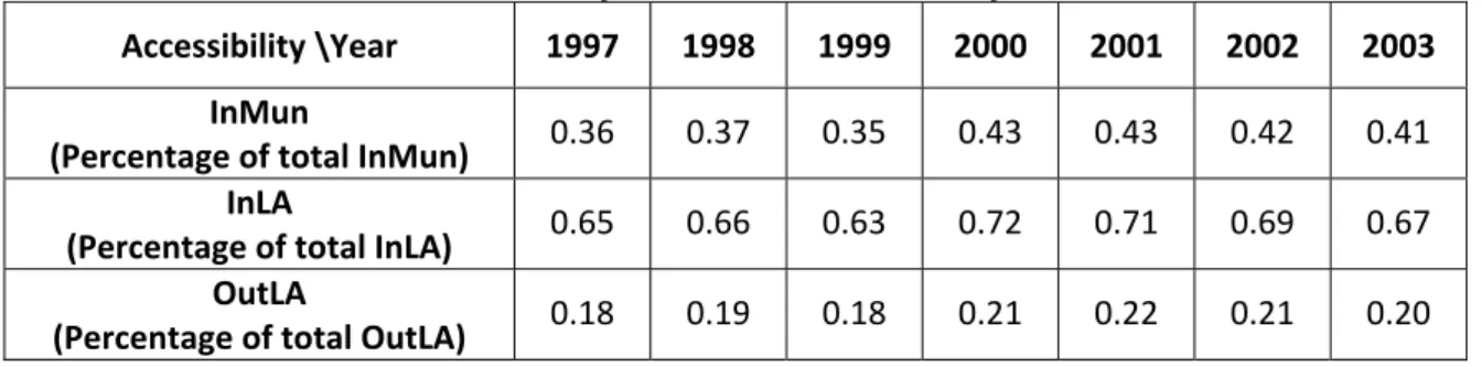
County\Year 1997 1998 1999 2000 2001 2002 2003 Mean labour productivity for municipalities in Stockholm County 73408 80139 78281 85615 87953 87448 88584 Mean labour productivity for municipalities in Västra Götaland County 65713 69053 71240 75050 75874 76934 79197 Table 2.2 and Table 2.3 compares import accessibility values between Stockholm and Västra Götaland. For example, added together, the municipalities in Stockholm County have an import accessibility value for InMun equal to 36 percent of the total import accessibility value for InMun in Sweden in 1997. However, comparing the two counties Stockholm has a high share of accessibility to imports for InMun and an even higher share of accessibility to imports for InLA compared to Västra Götaland. The significant difference between the two means that Stockholm has a high accessibility to imports rate to the surrounding area

(13)

8

confirming that Stockholm County has a high knowledge base assuming that imports contain knowledge.

Table 2.2 Accessibility for Stockholm County

Accessibility \Year 1997 1998 1999 2000 2001 2002 2003 InMun (Percentage of total InMun) 0.36 0.37 0.35 0.43 0.43 0.42 0.41 InLA (Percentage of total InLA) 0.65 0.66 0.63 0.72 0.71 0.69 0.67 OutLA (Percentage of total OutLA) 0.18 0.19 0.18 0.21 0.22 0.21 0.20

Table 2.3 Accessibility for Västra Götaland County

Accessibility \Year 1997 1998 1999 2000 2001 2002 2003 InMun (Percentage of total InMun) 0.20 0.20 0.22 0.20 0.22 0.24 0.25 InLA (Percentage of total InLA) 0.17 0.08 0.18 0.15 0.16 0.19 0.20 OutLA (Percentage of total OutLA) 0.25 0.25 0.27 0.26 0.28 0.30 0.31

2.4 Import Replacement and Imitation

Basic trade theory states that when exports increase wealth increases because additional exports mean higher revenues ceteris paribus (Bade and Parkin, 2004). The same is true for firms. They “export”, sell products from their stock to gain revenues. However, imports can be shown to generate an even larger positive effect than exports through stimulation of local productivity. To see why, imports flows should be analysed dynamically without applying the ceteris paribus condition and instead examine the question; what are the real effects generated by changing the composition of imports? Before doing this the following assumptions based on Jacobs (1969), Jacobs (1985) and SOU 1990:34 are presented:

(14)

9

• Imports alone does not cause productivity to change • A potential market for the imported product must exist

• Knowledge of the product allowing for local production must exist • Imports are paid for using revenue from exports

Jacobs (1985) differentiates between two kinds of cities, the import‐replacing city and the backward city. The import‐replacing city will substitute its imports with local production. This is done mostly by imitating imported goods but also through production of new products using the imported goods as a basic blueprint to build on. This type of city promotes economic growth in the long run. By replacing imports with locally produced goods, a city becomes innovative and is able produce products for export to other regions that can be sustained over time (the process is explained in more detail later in this section). If a city is not an import‐replacing city it is called a backward city (Jacobs, 1985). It is recognized by its high dependency on one or two major commodities which are not enough to spur economic activity in the long run. Being dependant on one or two commodities makes a city extremely vulnerable to changes in market conditions related to these products. Backward cities should because of this strive to become import‐replacing cities and trade heavily with other backward cities to create a more diversified range of products. Trade with import‐replacing cities should merely be used as a springboard and not as a constant source of trade. Otherwise, the bridge between what they can produce and what they import becomes too large. This will reduce the vulnerability on one or two major markets and is vital during the transition from being a backward city to becoming an import‐replacing city.

Jacobs (1969) provides a simple mathematical formula for the import‐replacing process described above:

• D nTE A nD

(D stands for division of labour, nTE for trial and error and A for a new activity. This process leads to nD which stands for the new divisions of labour)

In this process, trial and error plays an important role. The more trial and error the more successful products will be developed and it ensures that niches arise which ensures

(15)

10

diversity. If the demand for one product decreases or stops completely, other sources of revenue can still be relied on for securing jobs and development.

To give an example assume that chairs in City A previously had to be imported but is now going to be produced locally through imitation2. The new production of chairs means that more labour is needed for production in City (A) leading to new families settle down. The inhabitants of City A are now able to buy cheaper chairs than before (if the locally produced chairs were more expensive people would still import them), they have money left for additional consumption not previously afforded and City A now has a larger more competent workforce which is needed to effectively utilize the information from the imported goods (Johansson and Karlsson, 1991). This leads to city growth, both economically and population wise. After some time complement goods such as cushions or tables could are produced and in time exported to other cities generating revenues. This process generates positive effects on productivity levels in City A which has now done two things, imitated the production of chairs and created complements, which has lead to additional revenue leaving the city better off. Jacobs (1969) argues that this kind of growth is vital for a city and is in fact the backbone of city’s development.

This discussion can be connected to Marshall’s (1920) three prerequisites for clusters. Producing a variety of goods will lead to the creation of a skilful labour pool, as the number of firms in a city increases the level of technological spillovers will also increase and as a city experiences growth local non traded inputs increase which is consistent with the prerequisites for cluster formation presented in section 2.3.

Given this it is reasonable to assume that cities develop differently through time making them virtually unique. By analyzing the composition of imports of goods and services, these differences can be found. The type of import depends on the kind of demand and since cities are different, the composition of goods imported must also be “unique” for every city. 2_{Imports are likely to be imitated (SOU, 1990:34; Jacobs, 1985) due to two reasons. First, these products are} fully functioning and second, there is a market for them proven by the fact that they are imported.

(16)

11

2.5 Summary

and

Hypothesis

Imports and labour productivity levels are connected at the regional level. Accessibility is a proximity variable measuring geographical proximity and applied to imports to measure its relationship to labour productivity levels. These imported goods should be seen as sources of knowledge which are used to improve existing production or help to create completely new goods and in the process affecting productivity levels. Imports are usually imitated for local production and require more workers leading to the creation of new jobs. Cities were used as a frame to analyse the dynamics between imports and labour productivity to easier understand how labour productivity in municipalities is affected by imports. Based on the theory presented in this chapter the following hypotheses are stated: H1: There is a positive relationship between import accessibility and labour productivity. The theory presented implies a positive relationship between labour productivity and imported goods. Embodied knowledge in goods are used to improve production of existing products or used to produce a new product. Product variation is a key factor in understanding this relationship because the more variation the more differentiated knowledge is available. The theory presented advocates a relationship between imports and imported goods but also recognize that there are more factors influencing labour productivity.

(17)

12

3 Empirical

Analysis

This chapter outlines the empirical framework used in this thesis. The variables included are presented and the regression outputs are analyzed.

3.1 Regression

Model

The regression model estimated in this master thesis will be built to that of Fingleton (2001). This model is presented here in (1) for easy comparison. (1) 3: Where: = Exponential growth rate of final good productivity = Rate of productivity growth in neighbouring regions, captures a spillover effect = Exponential growth rate of final good output = Technological gap between the leading region and the rest = Urbanization level

= Distance to a central point (Taking Sweden as an example, the central point would be Stockholm)

This model is used as a point of reference. The productivity variable is redefined in (2). The variables and are removed from the model and import accessibility variables are added instead because they measure the relationship between productivity and import exposure. Using the accessibility variables, and do not add significant information. , and will be left in the model. Finally, a time variable is added to see how labour productivity changes over time. These changes make it an additive model instead of a multiplicative model.

3_{The explanation of the variables of the regression model Equation (1) is kept at a minimum. For further}

(18)

13

Salaries and employment levels are used to define the labour productivity variable. If salary is seen as the product of an individual’s productivity then high productivity yields a high salary and low productivity yields a low salary. The labour productivity in municipality i is calculated in (2).

(2): =

Where denotes wages in municipality i at time t, denotes employment in municipality i at time t and denotes labour productivity in municipality i at time t.

To capture the effect imports have on labour productivity, import accessibility variables measured in terms of total value are introduced to the model and presented in (4)

(4):

where denotes local accessibility to imports, intra regional accessibility to imports and inter regional accessibility to imports as presented in Chapter 2. The time variable denoted T measures the effect of time. Each municipality (289 included) is given a number from 1 to 289 to measure the effect of time between 1997 and 2003. The data used for the regression model is both cross‐sectional and time series data. The final model is attained in (5). (5): 1 2 3 Where: = Labour productivity in municipality i at time t = Intra municipality import accessibility in municipality i at time t = Intra regional import accessibility for municipality i at time t = Inter regional import accessibility for municipality i at time t

(19)

14 = Technological gap4 between the leading municipality and municipality i at time t = Population density in municipality i (in km2) at time t = Distance to Stockholm in kilometres from municipality i = Time = Normally distributed error term => E ~ 0, Data for the time period 1997‐2003 has been collected for testing. No data for wages 1997 was available instead wages for 1996 was applied as a substitute. The data is collected in nominal values and a consumer price index (SCB, A) with base year 1980 is used to deflate these values. There are 289 municipalities included in the sample, all municipalities existing during the time period chosen. A complete list is included in Appendix 2. The data used is both cross‐sectional and time series making the data pooled (Gujarati, 2003). A constraint on the type of imported products is applied using the Swedish Standard Industrial Classification, SNI92 (SCB, B). With the exception of SNI 11, 12, 13, 14 and 23 the product groups 1‐38 are used. The groups were selected to remove services from the data. Products that contain a small amount of embodied knowledge such as natural gas, oil and ore were also removed. The selected groups include products with higher level of embodied knowledge such as electronics and household appliances.

4_{Technological Gap is calculated using the following equation:}

Productivity in the municipality with the highest productivity – productivity in municipality i = Technology gap for municipality i.

(20)

15

3.2 Descriptive

Data

Table 3.1 shows for comparison reasons descriptive data for labour productivity in 1997 and 2003. The mean value for labour productivity has increased substantially comparing the values for 1997 and 2003. The same is true for the median values indicating stable growth during the time period. The min value 0 for labour productivity in 1997 is there because Nykvarn was created during the time period chosen. However, the min and max values have also increased during 1997 to 2003 as expected when looking closer at mean and median values.

Table 3.1 Descriptive Statistics for Labour Productivity

Variable Mean Median Min Max

Labour Productivity 1997 67519.09 67009.50 0 90267.06

Labour Productivity 2003 80603.46 79886.14 63017.37 116411.2

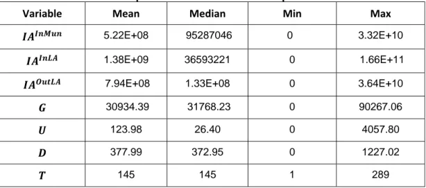
The descriptive statistics for the independent variables is presented in Table 3.2 but does not include a comparison between 1998 and 2003 as for labour productivity. Table 3.4 presents an overview of the variables to determine characteristics. The accessibility variables and Population Density does not have bell shaped characteristics and are skewed to the left which is seen by looking at the mean, median, min and max values for these variables. Technology Gap and Distance to Stockholm on the other hand do have bell shaped characteristics. Time is somewhat different because the descriptive statistics describes the values given to the municipalities (1 to 289) making median and mean value the same.

(21)

16

Table 3.2 Descriptive Statistics for the Independent Variables

Variable Mean Median Min Max

5.22E+08 95287046 0 3.32E+10

1.38E+09 36593221 0 1.66E+11

7.94E+08 1.33E+08 0 3.64E+10

30934.39 31768.23 0 90267.06 123.98 26.40 0 4057.80 377.99 372.95 0 1227.02 145 145 1 289 Table 3.1 provides an overview of the effect the independent variables are expected to have on the dependent variable.

Table 3.3 Independent Variables

Variable Effect on dependent variable Local import accessibility ( ) Positive Intra regional import accessibility ( ) Positive Inter regional import accessibility ( ) Negative Technological gap ( ) Negative Population density ( ) Positive Distance to Stockholm ( ) Negative Time ( ) Positive

Out of the accessibility variables, and are expected to have a positive effect on labour productivity and a negative. This is due to competition. Outside the LA‐region to which municipality i belongs to there are other municipalities that have a higher accessibility to imports due to their proximity (Johansson, Klaesson and Olsson, 2002). The result is that is expected to have a negative effect on the dependent variable. The correlation matrix in Table 3.4 presents the correlation between the variables used.

(22)

17

Table 3.4 Correlation Matrix 1

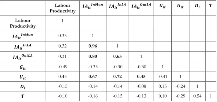
Labour Productivity Labour Productivity 1 0.35 1 0.32 0.96 1 0.31 0.80 0.65 1 -0.49 -0.33 -0.30 -0.30 1 0.43 0.67 0.72 0.45 -0.41 1 -0.15 -0.14 -0.14 -0.08 0.15 -0.24 1 -0.10 -0.16 -0.15 -0.13 0.10 -0.29 0.54 1 There is a fairly low correlation between the dependent variable labour productivity and the independent variables of which the highest correlation is 0.49. The import accessibility variables have a correlation to population density equal to 0.67, 0.72 and 0.45 respectively. However, the main problem in the data set is the correlation between the accessibility variables. The correlation matrix in Table 3.4 shows a correlation of 0.94, 0.97 and 0.87 between these variables, values extremely close to perfect multicollinearity. This high correlation between variables is a strong indicator of a problem with multicollinearity. Estimating the regression model as presented in section 3.1 results in that the output values for , and becomes indistinguishable and the individual impacts on labour productivity cannot be determined (Gujarati, 2003). Further, the expected effect of the independent variables on the dependent variable does not coincide with the signs in Table 3.4. Due to this the regression will also be tested using total accessibility5 denoted Total Acc instead of applying the accessibility variables separately. The correlation matrix in Table 3.5 includes total accessibility and shows that the problem of extreme collinearity in the data is no longer present. The variable time still has a negative sign showing that there still is collinearity in the data. 5_{Total Accessibility:}

(23)

18

Table 3.5 Correlation Matrix 2

Labour Productivity Labour Productivity 1 0.34 1 -0.49 -0.32 1 0.43 0.70 -0.41 1 -0.15 -0.14 0.15 -0.24 1 -0.10 -0.16 0.10 -0.29 0.54 1 This model is stated in (6). (6)

In addition, the model will be tested using different combinations of the accessibility variables such as only applying in the regression. By testing different combinations of the model it is possible to determine which one is the most correct taking collinearity into account.

(24)

19

3.3 Analysis

Table 3.6 and Table 3.7 show regression outputs from eight regressions using different combinations of the import accessibility variables including R2 and F‐values. The regressions are all tested using pooled least squares instead of a panel to get better results taking collinearity into account.

Table 3.6 shows the output from the original model defined in section 3.1 as well as three outputs where only one of the accessibility variables are used in each regression. All the variables as well as the F‐values in all regressions are significant as seen by the t‐values. However, in Output 1 and 4 the expected effects of and on the dependent variable respectively, are different from the expected effect confirming that there is a problem with collinearity (Gujarati, 2003). The R2 value in the outputs is 0.31 or 0.32. Output 2 and 3 have significant variables and show the expected effect on labour productivity on all variables.

Table 3.6 Regression Outputs, Summary Table A

Dependent Variable:

Labour Productivity Output 1 Output 2 Output 3 Output 4

2.56E‐06 (13.17) 3.77E‐07 (7.81) ‐5.08E‐07 (‐14.22) 2.41E‐08 (2.10) ‐1.82E‐07 (‐3.05) 3.70E‐07 (10.98) Total Accessibility Technological Gap ‐0.33 (‐43.69) ‐0.36 (‐40.68) ‐0.37 (‐41.36) ‐0.35 (‐39.55) Density 6.44 (26.46) 4.67 (17.77) 5.52 (19.32) 5.05 (22.75) Distance to Stockholm ‐2.20 (‐6.65) ‐2.18 (‐5.53) ‐2.16 (‐5.46) ‐2.35 (‐5.97) Time 5.56 (6.06) 4.17 (3.82) 4.35 (3.96) 4.79 (4.41) R2 0.32 0.31 0.31 0.31 F‐Value 967.94 908.41 892.11 925.61 Method: Pooled Least Squares t‐statistics within brackets

(25)

20

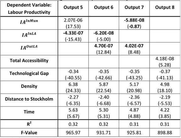
Table 3.7 show regression outputs using two or more accessibility variable in each regression and finally an output where total accessibility is used. Outputs 5, 6 and 7 shows the problem of collinearity in the data more clearly. Even though one of the accessibility variables has been removed from the model the signs in each regression still show that the collinearity is a problem and in Output 7 is not significant. Output 8 show significant results for all variables and the variables have the expected effect on the dependent variable. The R2 value of 0.31 is not significantly lower than in the rest of the outputs, it lies steady on 0.31 or 0.32. Due to these findings regression output 8 is found to be most accurate. It includes the three accessibility levels and yields expected output results. Although time showed to have a negative effect on the dependent variable in Table 3.5 the output shows it to have a positive effect as confirmed by all output presented in the Table 3.6 and Table 3.7.

Table 3.7 Regression Outputs, Summary Table B

Dependent Variable:

Labour Productivity Output 5 Output 6 Output 7 Output 8

2.07E‐06 (17.53) ‐5.88E‐08 (‐0.87) ‐4.33E‐07 (‐15.43) ‐6.20E‐08 (‐5.00) 4.70E‐07 (12.84) 4.02E‐07 (8.48) Total Accessibility 4.18E‐08 (5.28) Technological Gap ‐0.34 (‐40.55) ‐0.35 (‐42.66) ‐0.35 (‐43.25) ‐0.37 (‐41.13) Density 6.38 (24.33) 5.87 (22.54) 5.17 (20.98) 4.98 (18.10) Distance to Stockholm ‐2.27 (‐6.35) ‐2.40 (‐6.68) ‐2.36 (‐6.57) ‐2.19 (‐5.53) Time 5.63 (5.67) 5.30 (5.31) 4.87 (4.88) 4.22 (3.85) R2 0.32 0.32 0.31 0.31 F‐Value 965.97 931.71 925.81 898.88

Method: Pooled Least Squares t-statistics within brackets

Total import accessibility shows a positive effect on labour productivity which is expected. The inflow of knowledge stored in imported products should generate positive effects on

(26)

21 labour productivity as the output result confirm. The effect on labour productivity is small. This could be due to the small changes in import accessibility in the chosen time period. Technological gap shows a negative effect on productivity. It is an expected result as an increase in the gap should affect labour productivity levels negatively. Population density has a positive effect on the dependent variable productivity as expected. As more people settle down overall productivity levels should increase because more people are included in the production process leading to higher overall productivity. Distance to Stockholm has the expected negative effect on productivity. The further away from Stockholm a municipality is located the less advantage it has. Stockholm as the number one primal city in Sweden generates positive effects on surrounding municipalities which decreases with distance. Time itself has a positive effect on productivity. As time goes by new production methods are used and new inputs in the production are used. It stands to good reason as when R&D makes progress over time so should productivity levels. Looking at the R2‐value, 31 percent of the variation in Y can be explained by the independent variables. The F‐value is highly significant which means that the independent variables influence the dependent variable productivity and they are significant for the regression. The hypothesis stated in the end of Chapter 2 can now be answered. There is a positive relationship between the variables total import accessibility and labour productivity. Goods imported at the municipal level can therefore be concluded to affect labour productivity at the municipal level in Sweden.

(27)

22

Conclusion

The regression output shows that all variables chosen are significant and thereby have an effect on labour productivity. Labour productivity levels are affected by how many individuals contributing. By using the variable Population Density in the model it was possible to estimate the general efficiency of Sweden’s workforce. When population density increases by 1 unit labour productivity increases by 4.98 units.

Time itself generates positive effects on labour productivity as the regression result confirms. Jacobs (1969) stated that the most important aspect in creating a new product is trial and error. As time goes by, an increasing amount of trial and error results in positive effects (in this case to labour productivity). The variable Time also functions as a variable that registers any residual effects on productivity that is not accounted for by the other variables similar to the error term with the exception that whatever factor contributing to changes in labour productivity it is also affected by the constraint time.

However, Technology Gap and Distance to Stockholm are more interesting to analyze due to the theory behind them. Linking Technology Gap to Jacobs’s (1969) reasoning about backward and import replacing cities is interesting because of the time difference between now and then. Can Sweden today be fitted into her theory from 40 years ago? Distance to Stockholm tells us that the city Stockholm is important to the labour productivity levels across the country which also allows for interesting conclusions.

Jacobs (1985) wrote that to close the gap between being a backward city and being an import‐replacing city, backward cities should trade the most with one another because trading with an import‐replacing city does not help due to the gap itself. The gap makes the backward city unable to utilize goods for internal production. As seen in Table 3.5 Technology Gap has a negative effect on labour productivity (‐0.37). This result does not contradict Jacobs (1985), however, today technology is more widespread throughout Sweden compared to 20 years ago and there is probably a smaller gap in technology between municipalities and between cities generally speaking which could explain the low effect on labour productivity. Technology Gap would likely have a larger effect on the dependent variable if countries were compared instead of municipalities because the

(28)

23

difference in technology levels between countries in the world are generally larger. However, the distinction between the backward and the import‐replacing city is applicable in Sweden today. There are plenty of smaller cities that would not survive financially on their own which is also true for municipalities. Technology gap is therefore an important factor that affects productivity levels as showed by the significant result of the variable Technology Gap.

The Distance to Stockholm also has a negative effect on labour productivity which is not surprising. It tells us about the importance of Stockholm as a city in Sweden. It generates positive effect on labour productivity outside the city. This variable measures the distance from the municipalities in Sweden to the central point Stockholm. It takes into account that Stockholm is the number one primal city in Sweden. Section 2.3 provided data for Stockholm County concluding the importance of this region in terms of labour productivity rates and accessibility to imports. The significant t‐statistic shows that the further away from Stockholm a municipality is located the less positive spillover effect is generated towards that municipality. A municipality needs to be located close to Stockholm to utilize any spillover effect.

Total import accessibility is significant and shows a small effect on the dependent variable. The model was re‐specified to deal with a problem of near perfect multicollinearity which is a finding in itself. The multicollinearity problem made it impossible to decide to what to extent local, intra or inter accessibility effects labour productivity. Import accessibility applied on an additive model should not be used divided up into levels.

The significant t‐statistic also means that the theory in Chapter 2 of how import accessibility effects labour productivity holds true. It is correct to say that goods that are imported goods contain knowledge which can be used to improve existing products or create new products. The knowledge inflow to municipality i is connected to imported goods to municipality i. However, the R2‐ value of 0.31 implies that there are other factors that affect productivity and the knowledge inflow. For example Strömquist (1998) suggests that education is a source for knowledge. The level of education of a workforce is an important factor in deciding productivity levels. Basic education (12th grade) helps to create the workforce and

(29)

24

higher education (university) gives it higher human know‐how. Education helps the workforce to utilize the knowledge from the imported goods and should contribute to labour productivity. However, the regression output shows that import accessibility does affect labour productivity.

In conclusion, there were significant results for all variables included. Technology Gap and Distance to Stockholm has a negative effect on labour productivity and Population Density and Time has a positive effect on labour productivity. The import accessibility variables local, intra and inter accessibility were added together to measure total accessibility to remedy the high multicollinearity problem. The output results show that import accessibility affect the dependent variable which answers the purpose of this thesis to estimate if the municipal import value levels effect labour productivity.

There are several other studies to be done in the area. First, instead of analysing how productivity is affected by imports, using productivity growth as the dependent variable might yield different results. It is also a good idea to change the way in which the dependent variable is calculated. Here it is based on salaries and employment rates but using a different calculation method might yield different results. Second, increase the years included in the regression, perhaps using ten years instead of 6. Third, it would be interesting to compare different time periods e.g. 1980‐1989 and 2000‐2009. The world has changed a lot in the past 20 years. Making the comparison would therefore be even more interesting in this case. However, this means that the data collection will be massive, especially to calculate for the accessibility variables. Fourth, use different additional variables to the accessibility variables e.g. accessibility to labour. It would also be interesting to use lagged values of the dependent variable as an independent variable. Productivity levels of previous years might affect the productivity level in the current year.

(30)

25

Literature List

Andersson, M. and Karlsson, C., 2004. The role of accessibility for the performance of regional innovation systems. Knowledge Spillovers and Knowledge Management. pp. 283‐ 311. Bade, R. and Parkin, M. 2004. Foundations of Macroeconomics. 2nd ed. Boston: Pearson Addison‐Wesley. Baptista, R., 2003. Productivity and the density of local clusters. In J. Bröcker, D. Dohse & R. Soltwedel, Ed. Innovation clusters and interregional competition. Berlin: Springer, 2003, pp. 163‐181. Dixit, A.K. and Stiglitz, J.E., 1977. Monopolistic competition and optimum product diversity. In M. Greenhut and G. Norman, Ed. The economics of location. Vol.3, Spatial microeconomics. Aldershot: Elgar, 1995, pp. 284‐295. Fingleton, B., 2001. Equilibrium and economic growth: Spatial econometric models and simulations. Journal of Regional Science, 41(1), pp. 117‐147. Gujarati, N.D., 2003. Basic econometrics. 4th ed. Boston: McGraw Hill. Halpern, L., Koren, M. and Szeidl, A., 2006. Imports and Productivity. mimeo, Federal Reserve Bank of New York. Jacobs, J., 1969. The economy of cities. New York: Random house, Inc. Jacobs, J., 1985. Cities and the wealth of nations: principles of economic life. New York: Vintage Books. Johansson, B. and Karlsson, C., 1991. Från brukssamhällets exportnät till kunskapssamhällets innovations nät. Karlstad: Länsstyrenlsen i Värmlands län i samarbete med Högskolan I Karlstad. Johansson, B. Klaesson, J. and Olsson, M., 2002. Time distance and labour market integration. Papers in regional science, 81. pp, 305‐327. Keller, W., 2000. Do Trade Patterns and Technology Flows Affect Productivity Growth? The International Bank for Reconstruction and Development: The World Bank. Keller, W. 2002. Technology Diffusion and the World Distribution of Income. Brown University and University of Texas. Marshall, A., 1920. Principles of economics: an introductory volume. London: Macmillan. McCann, P., 2001. Urban and Regional Economics. New York: Oxford University Press Inc.

(31)

26 Romer, P.M., 1986. Incresing returns and long‐run growth. The economics of productivity. Vol. 2, Cheltenham: Elgar, 1997, pp. 174‐209. Romer, P.M., 1990. Endogenous technological change. In E. Mansfield & E Mansfield, Ed. The economics of technical change. Aldershot: Elgar, 1993, pp. 12‐43. (SCB, A), Statistics Sweden. (Updated: 2009‐02‐19) Consumer Price Index) [Online]. Available at: http://www.scb.se/Pages/TableAndChart____33848.aspx [Accessed 2 February 2009] (SCB, B), Statistiska Central Byrån. (Updated: 2008‐12‐02) SNI92, Rubriker, Aktivitetstexter och kommentarer, Sortering SNI92 [Online]. Available at: http://www.scb.se/Grupp/Hitta_statistik/Forsta_Statistik/Klassifikationer/_Dokument/sni92 _sni92sort.pdf [Accessed 3 February 2009] (SCB, C), Statistiska Central Byrån. (Updated: 2008‐11‐27) Län och kommuner i kodnummerordning [Online]. http://www.scb.se/Pages/List____257281.aspx [Accessed 8 February 2009] Smith, K,. 2000. What is the “knowledge economy”? Knowledge‐intense industries and distributed knowledge bases1. DRUID (Danish Research Unit for Industrial Dynamics), Summer Conference on The Learning Economy ‐ Firms, Regions and Nation Specific Institutions, Denmark 15‐17 June 2000. STEP Group: Norway. Statens Offentliga Utredningar, 1990:34, Statsregioner i Europa: underlagsrapport / av Storstadsutredningen. Stockholm: Allmänna förlag. Strömquist, U., 1998. Regioner, handel och tillväxt: Marknadskunskap för Stockholmsregionen. Stockholm: Regionplane‐ och trafikkontoret. Thangavelu, S.H. and Rajaguru, G. 2004. Is there an export or import‐led productivity growth in rapidly developing Asian countries? A multivariate VAR analysis. Applied Economics, 36, 1083–1093.

(32)

27

Appendix 1

Calculations for the import accessibility variables local, intra and inter accessibility. 1. exp 2. ∑ exp 3. ∑ exp 4. Where: = Import Accessibility to imports within municipality i.

= Import Accessibility to imports from within the LA‐region to which municipality i belongs to excluding municipality i.

= Import Accessibility to Imports from outside the LA‐region to which municipality i belongs to. = Total Import Accessibility in municipality i = Imports = Municipalities in municipality i: s LA‐region = Municipalities outside municipality i: s LA‐region = Time sensitive parameter = Distance between areas within municipality i.

= Time distance between municipality i and municipality r, where r represents municipalities within the LA‐region municipality i belongs to

= Time distance between municipality i and municipality e, where e represents municipalities outside the LA‐region to which municipality i belongs to.

(33)

28

Appendix 2

Table A1 Municipalities in Sweden

Upplands Väsby Linköping Vellinge Lerum Kristinehamn Gävle

Vallentuna Norrköping Östra Göinge Vårgårda Filipstad Sandviken Österåker Söderköping Örkelljunga Bollebygd Hagfors Söderhamn

Värmdö Motala Bjuv Grästorp Arvika Bollnäs

Järfälla Vadstena Kävlinge Essunga Säffle Hudiksvall

Ekerö Mjölby Lomma Karlsborg Lekeberg Ånge

Huddinge Aneby Svedala Gullspång Laxå Timrå

Botkyrka Gnosjö Skurup Tranemo Hallsberg Härnösand

Salem Mullsjö Sjöbo Bengtsfors Degerfors Sundsvall

Haninge Habo Hörby Mellerud Hällefors Kramfors

Tyresö Gislaved Höör Lilla Edet Ljusnarsberg Sollefteå

Upplands‐Bro Vaggeryd Tomelilla Mark Örebro Örnsköldsvik

Nykvarn Jönköping Bromölla Svenljunga Kumla Ragunda

Täby Nässjö Osby Herrljunga Askersund Bräcke

Danderyd Värnamo Perstorp Vara Karlskoga Krokom

Sollentuna Sävsjö Klippan Götene Nora Strömsund

Stockholm Vetlanda Åstorp Tibro Lindesberg Åre

Södertälje Eksjö Båstad Töreboda Skinnskatteberg Berg

Nacka Tranås Malmö Göteborg Surahammar Härjedalen

Sundbyberg Uppvidinge Lund Mölndal Heby Östersund

Solna Lessebo Landskrona Kungälv Kungsör Nordmaling

Lidingö Tingsryd Helsingborg Lysekil Hallstahammar Bjurholm

Vaxholm Alvesta Höganäs Uddevalla Norberg Vindeln

Norrtälje Älmhult Eslöv Strömstad Västerås Robertsfors

Sigtuna Markaryd Ystad Vänersborg Sala Norsjö

Nynäshamn Växjö Trelleborg Trollhättan Fagersta Malå

Håbo Ljungby Kristianstad Alingsås Köping Storuman

Älvkarleby Högsby Simrishamn Borås Arboga Sorsele

Tierp Torsås Ängelholm Ulricehamn Vansbro Dorotea

Uppsala Mörbylånga Hässleholm Åmål Malung‐Sälen Vännäs

Enköping Hultsfred Hylte Mariestad Gagnef Vilhelmina

Östhammar Mönsterås Halmstad Lidköping Leksand Åsele

Vingåker Emmaboda Laholm Skara Rättvik Umeå

Gnesta Kalmar Falkenberg Skövde Orsa Lycksele

Nyköping Nybro Varberg Hjo Älvdalen Skellefteå

Oxelösund Oskarshamn Kungsbacka Tidaholm Smedjebacken Arvidsjaur

Flen Västervik Härryda Falköping Mora Arjeplog

Katrineholm Vimmerby Partille Kil Falun Jokkmokk

Eskilstuna Borgholm Öckerö Eda Borlänge Överkalix

Strängnäs Gotland Stenungsund Torsby Säter Kalix

Trosa Olofström Tjörn Storfors Hedemora Övertorneå

Ödeshög Karlskrona Orust Hammarö Avesta Pajala

Ydre Ronneby Sotenäs Munkfors Ludvika Gällivare

Kinda Karlshamn Munkedal Forshaga Ockelbo Älvsbyn

(34)

29

Åtvidaberg Svalöv Dals‐Ed Årjäng Ovanåker Piteå

Finspång Staffanstorp Färgelanda Sunne Nordanstig Boden

Valdemarsvik Burlöv Ale Karlstad Ljusdal Haparanda

Kiruna

Table A2 Counties

Stockholm County Västra Götaland County

Upplands Väsby Härryda Töreboda

Vallentuna Partille Göteborg

Österåker Öckerö Mölndal

Värmdö Stenungsund Kungälv

Järfälla Tjörn Lysekil

Ekerö Orust Uddevalla

Huddinge Sotenäs Strömstad

Botkyrka Munkedal Vänersborg

Salem Tanum Trollhättan

Haninge Lerum Alingsås

Tyresö Vårgårda Borås

Upplands‐Bro Bollebygd Ulricehamn

Nykvarn Grästorp Åmål

Täby Essunga Mariestad

Danderyd Karlsborg Lidköping

Sollentuna Gullspång Skara

Stockholm Tranemo Skövde

Södertälje Bengtsfors Hjo

Nacka Mellerud Tidaholm

Sundbyberg Lilla Edet Falköping

Solna Mark Lidingö Svenljunga Vaxholm Herrljunga Norrtälje Vara Sigtuna Götene Nynäshamn Tibro (Source: SCB, C)