Mä lärdälen University
School of Innovätion Design änd Engineering
Vä sterä s, Sweden
Thesis for the Degree of Master of Science in Computer Science with
Specialization in Embedded Systems 15.0 credits
Analysing Real-Time Traffic in
Wormhole-Switched On-Chip
Networks
Shuyang Ding
dsg15002@student.mdh.se
Taodi Wu
twu15001@student.mdh.se
Supervisor: Meng Liu, Matthias Becker
Examiner: Thomas Nolte
May 25, 2016
Table of Contents
1. Introduction ... 1
2. Background and motivations ... 3
2.1 NoC structure... 3 2.2 NoC topologies ... 4 2.3 Wormhole Switching ... 4 2.4 XY-routing ... 5 2.5 Motivations ... 6 3. Problem Formulation ... 6 4. Related Work ... 7 5. Method ... 8 6. Expected Outcome ... 9 7. System model ... 9 8. Time Analysis ... 11
8.1 Analysis for round-robin based NoCs ... 11
8.2 Priority based analysis ... 14
9. Analysis Tool ... 21
10. Evaluation ... 24
10.1 Schedulability of different arbitrations ... 24
10.2 Schedulability of different numbers of virtual channels ... 26
10.3 Average WCTT ... 27
11. Conclusion ... 29
12. Future Work ... 30
Ackonwledgement ... 31
List of figures
Figure 1. Basic topology of bus-based communication model ... 2
Figure 2. An abstracted architecture of NoC ... 3
Figure 3. Regular Topologies Used in NoC [2] ... 4
Figure 4. Basic idea of wormhole switching ... 5
Figure 5. An example of building a path by XY-routing algorithm... 6
Figure 6. Research Method used in the thesis... 8
Figure 7. An example with five flows transmitting on a NoC ... 10
Figure 8. The graph of flow i over link k ... 12
Figure 9. User Interface of the Timing Analysis Tool ... 22
Figure 10. Random parameter set page ... 23
Figure 11. The timing tool after completed the analysis ... 24
Figure 12. The percentage of schedulable systems out of the total experiments for each setting ... 25
Figure 13. The schedulability ratio of shared priority based arbitration ... 26
Figure 14. The average WCTT over the number of hops for the packet size range [100,1000] ... 27
Figure 15. The average WCTT over the number of hops for different packet size ranges ... 28
List of tables
Table 1. Notations used in the analysis ... 9Table 2. Parameters for each flow in the example ... 10
Table 3. An example of input EXCEL file ... 22
Table 4. The percentage of schedulable systems out of the total experiments for each setting ... 25
Table 5. The comparison of schedulability ratio between RR and SP policy with different numbers of VC ... 26
Table 6. The number of flows for each policies ... 27
Table 7. The average WCTT over the number of hops for the packet size range [100, 1000] ... 28
Abstract
With the increasing demand of computation capabilities, many-core processors are gain-ing more and more attention. As a communication subsystem many-core processors, Network-on-Chip (NoC) draws a lot of attention in the related research fields. A NoC is used to deliver messages among different cores. For many applications, timeliness is of great importance, especially when the application has hard real-time requirements. Thus, the worst-case end-to-end delays of all the messages passing through a NoC should be concerned. Unfortunately, there is no existing analysis tool that can support multiple NoC architectures as well as provide a user-friendly interface.
This thesis focuses on a wormhole switched NoC using different arbitration policies which are Fixed Priority (FP) and Round Robin (RR) respectively. FP based arbitration policy includes distinct and shared priority based arbitration policies. We have developed a timing analysis tool targeting the above NoC designs. The Graphical User Interface (GUI) in the tool can simplify the operation of users. The tool takes characteristics of flow sets as input, and returns results regarding the worst-case end-to-end delay of each flow. These results can be used to assist the design of real-time applications on the corre-sponding platform.
A number of experiments have been generated to compare different arbitration mecha-nisms using the developed tool. The evaluation focuses on the effect of different param-eters including the number of flows and the number of virtual-channels in a NoC, and the number of hops of each flow. In the first set of experiment, we focus on the schedulabil-ity ratio achieved by different arbitration policies regarding the number of flows. The sec-ond set of experiments focus on the comparison between NoCs with different number of virtual-channels. In the last set of experiments, we compare different arbitration mecha-nisms with respect to the worst-case end-to-end latencies.
Keywords: network-on-chip, wormhole switching, fixed-priority, round robin,
1
1. Introduction
The structure of System-on-Chip (SoC) was proposed in early 1990s. SoC has long been utilized in the control field instead of generic computation field due to its insufficient computing power. Several approaches are widely used to improve the performance of SoC. One of them is to implement multi-core design which can obviously improve the performance with small buffering usage and relatively low frequency. The growth of the internal parallelism within the system results in the proposal of Multi-processors System-on-Chip (MPSoC).
MPSoC is a complex SoC integrating multiple processors on a single chip. It is designed based on many programmable processors and integrates most of or even all the re-quired resources [23]. The unit of the system is called a node which can be divided into computation node and communication node. The former one is utilized to achieve the goals of generalized computation. It can be a micro-processor or an Intellectual Property (IP) core. The other type of node and its links are responsible for the communication between the computation nodes. It can be bus, network or other communication infra-structure.
Bus is widely used as a way of interconnection in the early MPSoC field [23]. However, the defects of parallelism, efficiency and power consumption of bus have limited the de-velopment of MPSoC. As a result, NoC gains increasingly importance in the way of in-terconnection in MPSoC because it supplements the drawbacks of bus.
The basic topology of a bus-based communication is given in Figure 1. Bus-based ap-proach can present a small latency and good reusability. However, this model may not fulfill the requirements of these processors by providing the required bandwidth, latency and power consumption when the number of embedded cores increases. Thus an em-bedded switching network which is called Network-on-Chip is used to solve such com-munication bottleneck.
2 High Speed Bus
Low Speed Bus
I/O Bus Core Core Core Core Core Core Bus Bridge Bus Bridge
Figure 1. Basic topology of bus-based communication model
A NoC consists of a set of elements called routers and several channels interconnecting the cores. The cores need to access the routers to send or receive data. In many-core processors, each core is usually assigned with a router. The data generated by source node is sent to the destination node through one or more links between the routers [1]. Real-time analysis is a technique to describe the system runtime behaviour, which is usually performed at design phase of a real-time system. This technique is adopted to analyze the worst-case scenarios of NoCs. If a traffic-flow with the network latency in the worst case can meet its deadline, then the traffic-flow can meet its deadline for any other network latency situation. To help developers to design an appropriate NoC, this thesis aims to develop an analysis tool which integrates several analysis approaches corre-sponding with round-robin based and fixed-priority based NoC architectures. Further-more, a number of experiments are carried out in order to investigate how different net-work parameters can impact the quality of the real-time analyses.
In Section 2, the background and motivations are presented. The problem formulation of the thesis is described in Section 3 and related works are given in Section 4. The meth-od deployed in our thesis work is explained in Section 5. The outcomes we expected are listed in Section 6. Section 7 describes the system model in details. Time analysis comes next in Section 8. In Section 9, the developed analysis tool is introduced. Then Evaluation results are presented and discussed in Section 10. Finally we draw a conclu-sion and give some ideals about the future work in Section 11 and 12.
3
2. Background and motivations
NoC is a communication subsystem used in SoC in general. In addition, NoC technology can bring notable improvements over conventional bus and crossbar interconnection. It can also improve the scalability of SoC as it applies networking theory and methods to on-chip communication. An overview of NoC is given in the following sub-sections.
2.1 NoC structure
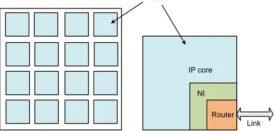
A number of network units which we call nodes are interconnected by routers in NoC. A node is composed of an IP core, a router and the corresponding network interface (NI) or network adaptor (NA). Figure 2 basically depicts a NoC structure involving 4×4 com-puting cores. The figure presents a simple 2D-mesh based topology which is widely uti-lized in the research work as well as in the commercial market.
Router NI
IP core
Link Node
Figure 2. An abstracted architecture of NoC
Links play the first and most important role in NoC because they connect the nodes physically and implement the communication actually [2]. As shown in Figure 2, the dou-ble arrowed line represents the communication links which consist of a set of wires. It connects adjacent routers by physically full-duplex channels. Routers with the implemen-tation of the communication protocols require a set of policies to deal with the packets collision, routing, arbitration etc. A router contains several input and output ports that are connected to shared NoC links and a switching matrix actually connecting the router inputs to its outputs. The switching matrix is not depicted in the figure. Besides, there is another local port to access the IP cores connected to this router. The third part is the NI or NA which logically builds connections between the IP cores and the network. Those IP cores may access the network by implementing different interface protocols. The IP core may have its own protocol with respect to a network, it is necessary to implement network adapter or network interface to make logic connection between them. In addition, computation and communication can be executed in parallel. This feature allows reuse of both core and communication independent of each other [4].
4
2.2 NoC topologies
A NoC is characterized by the physical structure on how the routers are connected. This structure is called topology. Many topologies used in NoC greatly refer to the computer networks which are known as parallel computer network architectures. But NoC has its own features. A topology in NoC defines how the nodes are interconnected with each other and how the links are deployed. It significantly influences the traffic delay of mes-sage flows, throughput, fault tolerance and power consumption etc.
Figure 3. Regular Topologies Used in NoC [2]
For example, the graph on the left hand side in Figure 2 shows a simple 2D-mesh topol-ogy. Since each router is associated to a corresponding IP core, each pair can be seen as a node. Each node is connected to its neighbour nodes in the way how the topology is defined. Several widely used topologies are depicted in Figure 3.
As shown in Figure 3, the most common topologies are N-dimensional grid and the hy-percube. A message transmitting between two nodes may go though one or more inter-mediate nodes. It moves one direction at a time. Message communication is performed based on a specific routing algorithm implemented in the routers. The access to an out-put link of a router is controlled by an arbiter. Most considered arbitration mechanisms include round-robin based and fixed-priority based policies.
2.3 Wormhole Switching
The term switching in NoC defines how data is transmitted from source node to target node. In terms of packet-based (A packet is also called an instance of a message flow) switching approach, traditional methods can provide certain guaranteed throughput be-cause all flits (A flit is the smallest unit where the flow control is performed) in the packet will be sent as long as the header builds connection between routers. However these methods increase latency which tends to result in unschedulability. As a consequence, wormhole switching strategy [5] is proposed as it minimizes the communication latency
5
due to its principle. Each packet is divided into a number of fixed-size flits in the worm-hole network so that only small buffer is needed in each router to store these flits instead of storing a whole packet. This is because a router can start to transmit a received flit of a certain packet without waiting for the arrival of a complete packet.
head body body tail packet flits
tail body body head
flow
Figure 4. Basic idea of wormhole switching
As depicted in Figure 4, a packet is decomposed into four flits containing one head with routing information, two bodies with the payload data and one tail with the error checking information. Then all the flits are transmitted in pipeline fashion via each node. This re-sults in lower latency and larger throughput.
2.4 XY-routing
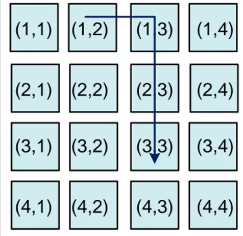
One of the significant factors that affect the communication efficiency of NoC is the rout-ing algorithm. A routrout-ing algorithm determines the path taken by a flow between its source node and destination node. The routing algorithms are commonly classified into deterministic and adaptive schemes. The XY-routing used in our analysis is a typical deterministic routing algorithm used in 2D-mesh based NoCs. It is easy to implement because it always selects the same path between a pair of nodes. For example in Figure 5, if the source node (denoted by (1, 2)) and destination node (denoted by (3, 3)) are given, the path built by XY-routing is shown as {(1, 2), (1, 3), (2, 3), (3, 3)}.The packet first goes along the horizontal direction towards its destination, and then turns to the ver-tical direction approaching its destination.
6
(1,1) (1,2) (1,3) (1,4) (2,1) (2,2) (2,3) (2,4) (3,1) (3,2) (3,3) (3,4) (4,1) (4,2) (4,3) (4,4)
Figure 5. An example of building a path by XY-routing algorithm
2.5 Motivations
As discussed in [3], in order to provide guarantees to real-time traffic over NoCs, there are two approaches commonly used as follows.
(1) Analyze the worst-case scenario traversal time of message flows;
(2) Modify hardware architecture in order to provide control of message transmissions. The first approach is widely utilized to guide the design of NoC due to its lower cost than the second one. There are a lot of approaches to analyze worst-case scenarios of NoC, but no existing analysis tool can support multiple NoC architectures and can provide convenient interactions with users.
Different real-time analysis schemes can achieve different performances for the same case. How to choose an appropriate approach to analyze a certain case is also very important to users’ design of a good communication solution. Thus, we will implement different methods for the same NoC arbitration to help designers to get a better timing analysis result of designed communication solution.
3. Problem Formulation
Considering two of the most commonly used NoC architectures which are RR based and FP based, a timing analysis tool with a friendly GUI needs to be developed. Users can set input parameters with appropriate configurations into the tool and get results of the worst-case traversal times. Users should also be able to select different NoC architec-tures as they want. The results can be used to guide the users to schedule real-time traffic over NoC.
Different analysis approaches have been proposed in the literature. However, each ap-proach typically has specific pros and cons which may not be suitable for all the cases. Therefore, in addition to the developed analysis tool, the main focus of this thesis is to compare multiple time analysis approaches regarding different NoC architecture policies. Based on the developed tool, a number of experiments need to be generated with the aim to investigate how different network parameters can impact the quality (including
7
accuracy and efficiency) of the timing analyses. The investigated parameters are listed below.
(1) Number of flows – The total number of message flows transmitting on the network. (2) Packet size – The size of each packet in flits (flow control unit, e.g. the smallest unit
of transmission in NoC).
(3) Utilization of the network – The usage of bandwidth for all the flows in the network. (4) Number of hops – The total number of links a flow traverses.
The derived observations or conclusions of these evaluations can help system designers to choose appropriate NoC configurations as well as suitable analysis approaches.
4. Related Work
In this work, we focus on the priority based and round-robin based wormhole switching policies.
Several approaches have been proposed to analyze real-time traffic over NoCs. In [6], [7] and [8], worst-case network latency analysis approaches based on RR is proposed. Tar-geting a priority based wormhole switching technique, a number of timing analysis ap-proaches have been presented in [9], [10], [11] and [12].
NoC technology is proposed with the aim of handling the communication of multiple cores on a single chip. Based on this, a large amount of timing analysis with respect to NoC has been presented in the literature. A method of computation for worst-case delay analysis on a specific network named SpaceWire is presented in [6]. Some previous delay evaluation methods on wormhole networks have drawbacks like that they focused more on probabilistic results from which the network designers cannot get enough infor-mation. The authors propose a better approach in this paper that enables the determi-nation of an upper-bound on the worst-case end-to-end delay.
From the perspective of reducing average delay experienced by packets, Sethu and Shi [13] presents an Anchored Round Robin (ARR) scheduling strategy in wormhole strate-gy with Virtual Channel (VC). The stratestrate-gy maintains an anchor virtual channel where the scheduler returns when a flit is being served. Flits from other virtual channel cannot be served by the scheduler until the anchored virtual channel is empty. It is different from the traditional flit-by-flit round-robin strategy. A Recursive Calculus is proposed in [19] to compute the end-to-end delay for each flow. However, this approach does not take the period or the minimum inter-arrival time into account which may result in pessimistic es-timates. When the network utilization is relatively low, this pessimism may even get greater. Thus an improved analysis Tighter Recursive Calculus (TRC) [20] which can obtain tighter estimates is proposed.
In [14], the authors proposed a worst case network latency analysis scheme for real-time on-chip communication with wormhole switching and fixed-priority scheduling. The mod-el devmod-eloped in the paper can predict the packet transmission latency based on two quantifiable different delays: direct interference and indirect interference. The authors also proved that the exact determination of schedulability of a real-time traffic-flow set over the NoC is NP-hard when parallel interference exist.
8
In [26], the authors proposed a Stage-Level network latency analysis approach for the fixed-priority NoCs. A pipelined communication resource model is presented in [26], and the evaluation presented in the article shows that the approach can computer tighter network latencies than the analysis presented in [14]. However, this analysis assumes a large enough buffer on each router so that a flow can not be delayed because the next router in the path is full. Unfortunately, such a condition is not practical in NoCs.
The unique priority per traffic-flow implementation policy of the priority-based wormhole switching approach results in a high buffer cost and energy overhead. To solve this problem, Shi and Burns [15] proposed a shared priority policy. The policy allows multiple traffic-flows to contend for a single virtual channel and assign these traffic-flows the same priority. They also developed a composite model analysis scheme, which requires that the network latency is no more than the period of every traffic-flow. But under this restriction, it will get a large global delay when the approach is used to analyze a com-plex system. Therefore, Shi and Burns proposed an improved schedulability analysis scheme in [16] which can efficiently handle wormhole switching with a priority share poli-cy. Instead of computing the total time window for each traffic-flow, the new approach computes it at each priority level. This approach support flows with arbitrary deadlines, and it also achieves a lower computational complexity compared to the previous solu-tions.
5. Method
In this research, several real-time analysis methods are implemented in the analysis tool. Based on the tool, a number of experiments are developed to quantify the relationship between these features. Figure 6 shows the method we plan to use in the research. The analysis of observation can be used to revise the problem formulation, then start to next cycle of the research.
Figure 6. Research Method used in the thesis (1) Related Work Reading
To implement the evaluation and Graphic User Interface (GUI), it requires knowledge of the following topics and area:
Real-Time Analysis (RTA) Methods based on fixed-priority and round-robin Iterative RTA
Recursive Calculus GUI design and programming
Design principle for user interface
Programming techniques about Windows Presentation Foundation (WPF) (2) Implementation
9
A real-time analysis tool will be developed to analyse worst-case scenarios of NoCs, based on the tool, several evaluation experiments need to be generated. Five real-time analysis methods will be integrated into the analysis tool, then the evaluation experi-ments will be developed based on these analysis methods. We are going to implement the GUI by using WPF and the computation of analysis will be written in the C language. (3) Measurement and Observation
A number of timing analysis approaches will be implemented in the developed tool. After generating extensive experiments, we will investigate how different network parameters can impact the quality of different analysis approaches. According to the observation, the problem formulation can be revised and start an improved research.
6. Expected Outcome
The following main results are expected:
A developed analysis tool for NoCs with Graphical User Interface.
Extensive experiments to investigate the effects of given network parameters, and concluded observations for system designers.
7. System model
In this thesis, we consider systems with 𝑚 × 𝑚 computing cores, which is a typical de-sign used in most existing many-core implementations. An abstracted architecture of NoC is shown in Figure 2. The NoC uses a 4 × 4 2D-mesh based topology and the XY-routing principle which are simple to implement and widely utilized in both academic and commercial field. We consider two different arbitration schemes to access the output link at a certain router, which are round-robin arbitration and fixed-priority arbitration respec-tively. The purpose is to evaluate which scheme can obtain better performance from different perspectives.
Notations used in this paper are listed in Table 1:
Table 1. Notations used in the analysis
𝑏𝑤 The bandwidth of each physical link. In order to simplify the problem, we assume all the physical links use the same bandwidth.
𝜎 The size of a single flit.
𝑑𝑓 The transmission time of a single flit over a physical link(𝑖. 𝑒. 𝑑𝑓 = 𝜎 𝑏𝑤⁄ ). 𝐿𝑖 The packet size of 𝑓𝑖 which includes both of the header and payload.
𝐶𝑖 The basic transmission time of 𝑓𝑖 over one physical link(𝑖. 𝑒. 𝐶𝑖 = 𝐿𝑖⁄𝑏𝑤).
𝑇𝑖
The period of a periodic flow or the minimum inter-arrival time of a sporadic flow. That is to say, a new packet or instances is generated every 𝑇𝑖.
𝐷𝑖 The deadline which constrains the flow 𝑓𝑖. (𝐷𝑖 ≤ 𝑇𝑖)
𝑅𝑖 The fixed route of 𝑓𝑖.
10
ℱ = {𝑓1, 𝑓2 , … , 𝑓𝑛} is a set of 𝑛 periodic and sporadic flows which are transmitted in the
network. Each member in the set is characterized by a set of parameters denoted as {𝐿𝑖, 𝐶𝑖, 𝑇𝑖 , ℛ𝑖}. A flow is considered schedulable if 𝑅𝑇𝑖 is not greater than its
dead-line(𝑅𝑇𝑖 ≤ 𝐷𝑖). The whole network is considered schedulable if all the flows meet their
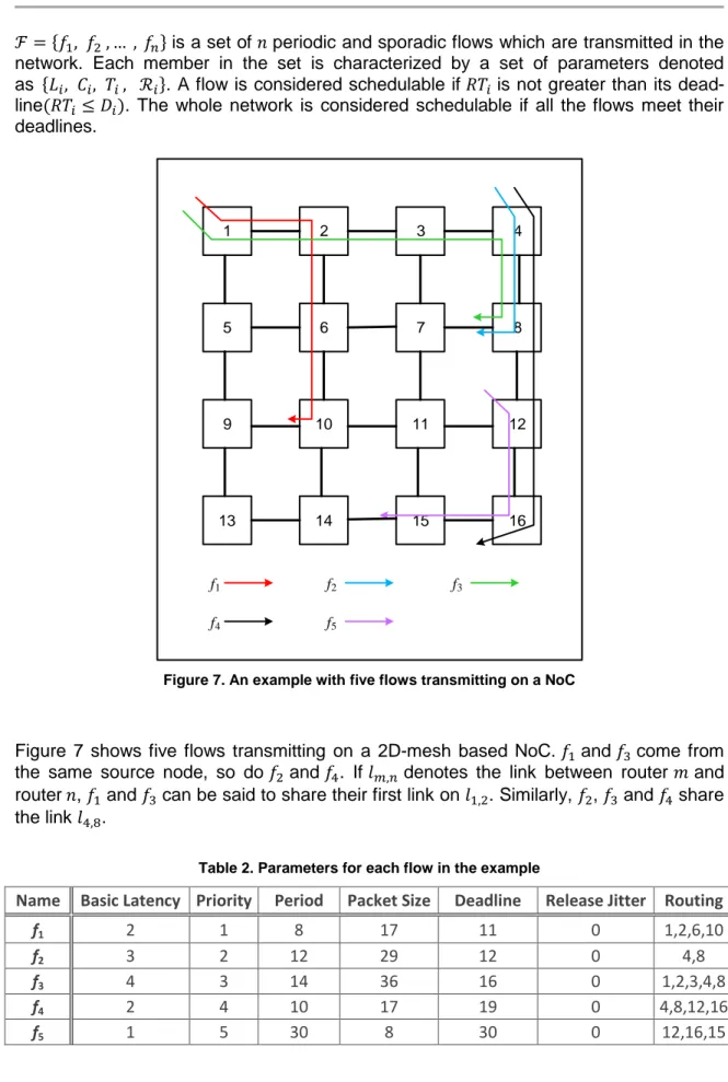
deadlines. 1 2 3 4 5 6 7 8 9 10 11 12 13 14 15 16 f1 f2 f3 f4 f5
Figure 7. An example with five flows transmitting on a NoC
Figure 7 shows five flows transmitting on a 2D-mesh based NoC. 𝑓1 and 𝑓3 come from
the same source node, so do 𝑓2 and 𝑓4. If 𝑙𝑚,𝑛 denotes the link between router 𝑚 and
router 𝑛, 𝑓1 and 𝑓3 can be said to share their first link on 𝑙1,2. Similarly, 𝑓2, 𝑓3 and 𝑓4 share
the link 𝑙4,8.
Table 2. Parameters for each flow in the example
Name Basic Latency Priority Period Packet Size Deadline Release Jitter Routing f1 2 1 8 17 11 0 1,2,6,10
f2 3 2 12 29 12 0 4,8
f3 4 3 14 36 16 0 1,2,3,4,8 f4 2 4 10 17 19 0 4,8,12,16 f5 1 5 30 8 30 0 12,16,15
11
8. Time Analysis
There are two stringent requirements in real-time applications, both correct result and timing. Targeting the real-time applications over the NoCs, the timing analysis is adopted to verify if all the time requirements can be satisfied. In this section,we present the tim-ing analyses for real-time communication in RR based and FP based NoCs.
8.1 Analysis for round-robin based NoCs
Due to the fact that a packet may pass through a number of routers in a wormhole-switched NoC, network calculus is not simple to compute the end-to-end delay of a packet over the NoC and may introduce significant pessimism [18]. Thus a Recursive Calculus (RC) based approach is proposed in [19]. However, this approach does not take the period or the minimum inter-arrival time into account which may result in pessi-mistic estimates. When the network utilization is relatively low, this pessimism may even get greater.
In order to guarantee the real-time performance, all the flows must be transmitted within a certain amount of time. Thus the idea of Worst-Case Transmission Time (WCTT) is introduced to check if all the flows can meet their deadlines.
Assume that 𝑓𝑖 is the flow under analysis. Obviously it is not easy to compute the
end-to-end delay of a packet of 𝑓𝑖 directly especially when it spans over multiple routers.
There-fore, the idea of computing the maximum delay on each link along its path (𝑅𝑖) arouses
the proposal of RC. A set of links 𝐿𝑖𝑛𝑘𝑖 = {𝑙𝑖1, 𝑙𝑖2, … , 𝑙𝑖 𝑛𝑖
} is used to denote all the links within 𝑅𝑖, where 𝑙𝑖1 is the first link while 𝑙𝑖
𝑛𝑖 is the last link. In other words, there are 𝑛
𝑖
links on the path of 𝑓𝑖 in total. 𝐷𝑒𝑙𝑎𝑦(𝑓𝑖, 𝑙𝑖𝑘) is the maximum delay of 𝑓𝑖 at a certain link
𝑙𝑖𝑘 (𝑙𝑖𝑘 ∈ 𝐿𝑖𝑛𝑘𝑖). The pseudo code in Algorithm 1 shows how 𝑑𝑒𝑙𝑎𝑦(𝑓𝑖, 𝑙𝑖𝑘) is calculated.
Algorithm 1 Original Recursive Calculus: Computing 𝑑𝑒𝑙𝑎𝑦(𝑓𝑖, 𝑙𝑖𝑘)
1 𝑑𝑒𝑙𝑎𝑦(𝑓𝑖, 𝑙𝑖𝑘) = 0;
2 for all 𝑙𝑥 that are upstream links next to 𝑙𝑖𝑘 and 𝑙𝑥! = 𝑙𝑖𝑘−1 .
3 { 𝑀𝑎𝑥𝐵𝑙𝑜𝑐𝑘𝑖𝑛𝑔 = 0
4 for 𝑓𝑗 coming from 𝑙𝑥 and going to the sharing link 𝑙𝑖𝑘
5 { if 𝑙𝑖𝑘 == 𝑙𝑗𝑛𝑗 /* 𝑙
𝑖𝑘 is the last link of 𝑓𝑗 */
6 𝑑𝑒𝑙𝑎𝑦𝐹𝑟𝑜𝑚𝑓𝑗= 𝐿𝑗/𝑏𝑤;
/* 𝑙𝑗𝑛𝑒𝑥𝑡_𝑙𝑖𝑘 is the downstream link next to 𝑙
𝑖 𝑘 on 𝑅 𝑗 */ 7 else 𝑑𝑒𝑙𝑎𝑦𝐹𝑟𝑜𝑚𝑓𝑗 = df + delay(𝑓𝑗, 𝑙𝑗 𝑛𝑒𝑥𝑡_𝑙𝑖𝑘 ) 8 𝑀𝑎𝑥𝐵𝑙𝑜𝑐𝑘𝑖𝑛𝑔 = 𝑀𝐴𝑋(𝑀𝑎𝑥𝐵𝑙𝑜𝑐𝑘𝑖𝑛𝑔, 𝑑𝑒𝑙𝑎𝑦𝐹𝑟𝑜𝑚𝑓𝑗); } 9 𝑑𝑒𝑙𝑎𝑦(𝑓𝑖, 𝑙𝑖𝑘)+= 𝑀𝑎𝑥𝐵𝑙𝑜𝑐𝑘𝑖𝑛𝑔; } 10 if 𝑙𝑖𝑘 == 𝑙𝑖𝑛𝑖 /* 𝑙
𝑖𝑘 is the last link of 𝑓𝑖 */
12 12 else 𝑑𝑒𝑙𝑎𝑦(𝑓𝑖, 𝑙𝑖𝑘)+= 𝑑𝑓 + 𝑑𝑒𝑙𝑎𝑦(𝑓𝑖, 𝑙𝑖𝑘+1) ; 13 return 𝑑𝑒𝑙𝑎𝑦(𝑓𝑖, 𝑙𝑖𝑘) ;
l
i kl
ik-1l
i k( )
Dr
l
i k( )
Sr
l
xl
ik+1f
iFigure 8. The graph of flow i over link k
Figure 8 illustrates how 𝑓𝑖 gets blocked when transmitted over the link 𝑙𝑖𝑘. As shown in
the figure, 𝑆𝑟(𝑙𝑖𝑘) and 𝐷𝑟(𝑙𝑖𝑘) represent the source and destination router of 𝑙𝑖𝑘 respec-tively. When computing the maximum delay of 𝑓𝑖 over 𝑙𝑖𝑘, not only the transmission time
of itself should be taken into account, flows who have pending packets in 𝑆𝑟(𝑙𝑖𝑘) and are
going to transmit over 𝑙𝑖𝑘 should also be considered. 𝑙𝑥 is one of the input links
(exclud-ing 𝑙𝑖𝑘−1 ) of 𝑆𝑟(𝑙𝑖𝑘). Flows coming from different input-links can cause blocking to 𝑓𝑖.
Each 𝑙𝑥 can at most transmit one packet ahead of 𝑓𝑖 according to RRA. Therefore, for a
certain 𝑙𝑥, where 𝐷𝑟(𝑙𝑥) = 𝑆𝑟(𝑙𝑖𝑘) , there might be several flows pending to transmit
through it. Only the flow that can cause the maximum blocking needs to be considered. For other input-links of the same type, the same operation can be performed by using a loop. In addition to the blocking caused by other flows, the flow may get blocked by itself because a complete packet are split into a number of flits and the flits are commonly spanned over multiple routers along its path (𝑖. 𝑒. 𝑅𝑖). In a wormhole-switching based
NoC, each router has a quite limited buffer that only holds several flits. Under such a situation, even if the flits of 𝑓𝑖 pending on 𝑆𝑟(𝑙𝑖𝑘) gets access to 𝑙𝑖𝑘, they will still be
blocked because there is no buffer capacity to store them. This is so-called back-pressure. Thus the delay from 𝑓𝑗 in this situation can be calculated by:
𝑑𝑒𝑙𝑎𝑦𝐹𝑟𝑜𝑚𝑓𝑗= 𝑑𝑓 + 𝑑𝑒𝑙𝑎𝑦(𝑓𝑗, 𝑙𝑗 𝑛𝑒𝑥𝑡_𝑙𝑖𝑘
) (1) Where 𝑓𝑗 is the flow coming from a certain 𝑙𝑥, 𝑙𝑗
𝑛𝑒𝑥𝑡_𝑙𝑖𝑘
is the next link of 𝑓𝑗 after the
shar-ing link 𝑙𝑖𝑘.
The explanation of Figure 7 above is mainly about two types of blocking to 𝑓𝑖 over 𝑙𝑖𝑘. It is
worth to notice that 𝑙𝑖𝑘 is neither the first nor the last link in 𝐿𝑖. On one hand, if 𝑙𝑖𝑘 is the
last link of 𝑓𝑖, meaning that the header of the packet has arrived at its destination. The
delay of 𝑓𝑖 over 𝑙𝑖𝑘 can be acquired by simply computing its transmission time (Algorithm
13
over a certain link is acquired. As we can see from Eq. (1), the maximum delay of 𝑓𝑖 over
𝑙𝑖𝑘 can be obtained by recursively computing the delays of a number of flows over the downstream links (Algorithm 1, line 4-7). The recursive process comes to an end until each flow finishes computing the delay over its last link. The 𝑅𝑇 of 𝑓𝑖 then can be
ac-quired by computing the largest delay over its first link (𝑑𝑒𝑙𝑎𝑦(𝑓𝑖, 𝑙𝑖1)) (Algorithm 2, line
1-4) as well as the delays of flows coming from the same source node (Algorithm 2, line 2-3).
Algorithm 2 Worst-case Traversing Time (WCTT): Computing 𝑊𝐶𝑇𝑇𝑖
1 𝑊𝐶𝑇𝑇𝑖= 𝑑𝑒𝑙𝑎𝑦(𝑓𝑖, 𝑙𝑖1);
/* No matter whether 𝑓𝑝 and 𝑓𝑖 share the first link */
2 for all 𝑓𝑝 that are emitted from the same source node
3 { 𝑊𝑖+= 𝑑𝑒𝑙𝑎𝑦(𝑓𝑝, 𝑙𝑝1) ;}
4 return 𝑊𝐶𝑇𝑇𝑖 ;
Example 1: considering the example presented in Section 7, we use the above
ap-proach to compute the 𝑅𝑇 of 𝑓4 . As we can see from Figure 6, 𝑓2 comes from the same
source node as 𝑓4. 𝑓4 shares a link which is known as 𝑙4,8 with 𝑓2 and 𝑓3, and it shares
link 𝑙12,16 with 𝑓5. To simplify the computation, 𝑑𝑓 is set to 1. The bandwidth in this
ex-ample is 10. The WCTT of 𝑓4 can be acquired by the following recursive computation.
𝑊4= 𝑑𝑒𝑙𝑎𝑦(𝑓4, 𝑙41) + 𝑑𝑒𝑙𝑎𝑦(𝑓2, 𝑙21) 𝑑𝑒𝑙𝑎𝑦(𝑓4, 𝑙41) = (𝑑𝑓 + 𝑑𝑒𝑙𝑎𝑦(𝑓3, 𝑙34)) + (𝑑𝑓 + 𝑑𝑒𝑙𝑎𝑦(𝑓4, 𝑙42)) = (𝑑𝑓 + 𝐿3⁄𝑏𝑤) + (𝑑𝑓 + 𝑑𝑒𝑙𝑎𝑦(𝑓4, 𝑙42)) 𝑑𝑒𝑙𝑎𝑦(𝑓2, 𝑙21) = (𝑑𝑓 + 𝐿2⁄𝑏𝑤) + (𝑑𝑓 + 𝑑𝑒𝑙𝑎𝑦(𝑓3, 𝑙34)) 𝑑𝑒𝑙𝑎𝑦(𝑓4, 𝑙42) = 𝑑𝑓 + 𝑑𝑒𝑙𝑎𝑦(𝑓4, 𝑙43) 𝑑𝑒𝑙𝑎𝑦(𝑓3, 𝑙34) = 𝐿3⁄𝑏𝑤 𝑑𝑒𝑙𝑎𝑦(𝑓4, 𝑙43) = 𝐿4⁄𝑏𝑤+ (𝑑𝑓 + 𝑑𝑒𝑙𝑎𝑦(𝑓5, 𝑙52)) 𝑑𝑒𝑙𝑎𝑦(𝑓5, 𝑙52) = 𝐿5⁄𝑏𝑤
Then substitute the values into the formulas above from bottom to up. 𝑑𝑒𝑙𝑎𝑦(𝑓5, 𝑙52) = 8 10⁄ = 0.8 𝑑𝑒𝑙𝑎𝑦(𝑓4, 𝑙43) = 17 10⁄ + (1 + 0.8) = 3.5 𝑑𝑒𝑙𝑎𝑦(𝑓3, 𝑙34) = 36 10⁄ = 3.6 𝑑𝑒𝑙𝑎𝑦(𝑓4, 𝑙42) = 1 + 3.6 =4.6 𝑑𝑒𝑙𝑎𝑦(𝑓2, 𝑙21) = (1 + 29 10⁄ ) + (1 + 4.6) = 9.5 𝑑𝑒𝑙𝑎𝑦(𝑓4, 𝑙41) = (1 + 3.6) + (1 + 4.6) = 10.2 𝑊4= 10.2 + 9.5 = 19.7
14
8.2 Priority based analysis
Two different priority based policies are discussed in this thesis, distinct priority policy and shared priority policy. For both policies, a simple introduction is presented, and also a worst case network latency analysis approach correspondingly.
8.2.1 Distinct priority policy
In [17], the authors present a flit-level preemptive wormhole switching method for mes-sage transmission. The method allows the mesmes-sages with higher priority to preempt the messages with lower priority between transmissions of different flits but not during the transmissions of a single flit.
For implementing this method, they introduce virtual channels which divide the resource of a single physical link into several logical separate channels with independent buffers [21]. Each of these buffers that can hold several flits of a packet is considered as a virtu-al channel. The virtuvirtu-al channels technique virtu-allows the blocking packet to be bypassed by a transmitting one. The virtual channels implementation can improve the utilisation of the network resource, and some traffic guarantees [22].
In the distinct priority policy, each priority level is assigned a virtual channel. A physical channel can contain several virtual channels. A virtual channel can obtain the physical channel if there is no higher virtual channel is active. A message with priority i can only request the virtual channel with priority i.
In [15], Shi and Burns propose a real-time communication analysis method for distinct priority based wormhole switching. In their communication model, each traffic-flow 𝑓𝑖 is
characterized by attributes 𝑓𝑖 = {𝑃𝑖 , 𝐶𝑖 , 𝑇𝑖 , 𝐷𝑖 , 𝐽𝑖𝑅 } . All the traffic-flows in the network are
periodically generated. 𝑃𝑖 is the priority of 𝑓𝑖 and distinct for each traffic-flow in the
net-work. All the packets belonging to the same traffic-flow inherit the priority of the flow. The value 1 denotes the highest priority, and the largest value denotes the lowest priority. 𝐶𝑖
is the basic network latency of 𝑓𝑖, which is calculated by:
i i L C H
bw
(2)Where, 𝐿𝑖 is the maximum packet size of 𝑓𝑖. 𝜎 denotes the size of a single flit. 𝐻
repre-sents the number of hops with in path of 𝑓𝑖. 𝑏𝑤 is the bandwidth of the link.
Each traffic-flow has a deadline 𝐷𝑖, which means all the packets which belong to the
traf-fic-flow should be delivered from a source router to the destination router within 𝐷𝑖 even
in the worst case. 𝑇𝑖 is the period of 𝑓𝑖 which represents the length of time between two
contiguous releases of successive packets. The release jitter 𝐽𝑖𝑅 denotes the maximum deviation of packets released from its period. For a packet from traffic-flow 𝑓𝑖, if it is
generated at time 𝑎, the release time will be no more than 𝑎 + 𝐽𝑖𝑅, and its absolute dead-line of this instance is 𝑎 + 𝐷𝑖. The basic network latency does not consider traffic-flow
contention, and this contention can extend the network latency of the packet. In the worst case analysis, the effects on network latency from competing intervention flows need to be evaluated based on inter-relationships between traffic-flows.
Under the priority arbitration policy, only traffic-flows with the higher priority than the cur-rent one can cause contention. Two kinds of interference are introduced in [17] to de-scribe the inter-relationship between the traffic-flows, direct interference and indirect
15
interference. Correspondingly, 𝑆𝑖𝐷 and 𝑆𝑖𝐼 are defined to denote the interference sets of
these two interferences on 𝑓𝑖. Let ℜ𝑖 denotes the routing of flow 𝑓𝑖, and 𝑒𝑚,𝑛 denotes the
link from router 𝑚 to router 𝑛. As the traffic-flow set presented in Section 7, routing of flow 𝑓𝑖 is ℜ1= {𝑒1,2, 𝑒2,6, 𝑒6,10}. The definitions of the two interferences are presented as
follows:
Direct interference: The higher priority traffic-flow shares at least one physical link with 𝑓𝑖, the set 𝑆𝑖𝐷 which contains all the higher priority traffic-flows which can force an
interference on 𝑓𝑖 directly is represented as:
,
D
i k k i k i
S f and P P f (3) Indirect Interference: The higher priority traffic-flow does not share any physical link with 𝑓𝑖 directly, but it shares physical link with the traffic-flows belong to direct
interfer-ence of 𝑓𝑖. The indirect interference set of 𝑓𝑖 can be represented as following:
, , ,
I D
i k k i j k k i j i k
S f and P P and f S f (4)
For each traffic-flow, the interference set 𝑆𝑖 which consists of all direct and indirect
inter-ference is defined as: 𝑆𝑖= 𝑆𝑖𝐷+ 𝑆𝑖𝐼. Note that, if a traffic-flow can cause both direct and
indirect interference, then the traffic-flow is only regarded as direct interference.
As the example shown in the Section 7, the priority of these traffic-flows can be assigned as 𝑃1= 1, 𝑃2= 2, … , 𝑃5= 5. Then the inter-relationship between the traffic-flows can be
derivated. 𝑓1 and 𝜏2 do not share any link with other higher priority traffic-flow, thus 𝑆1𝐷=
𝑆1𝐼= 𝑆2𝐷= 𝑆2𝐼 = ∅ and 𝑆1= 𝑆2 = ∅ . Traffic-flow 𝑓3 shares links with 𝑓1 and 𝑓2, 𝑆3𝐷=
{ 𝑓1, 𝑓2}, 𝑆3𝐼 = ∅, therefore 𝑆3= { 𝑓1, 𝑓2}. Traffic-flow 𝑓4 directly contends with 𝑓2 and 𝑓3
and indirectly contends with 𝑓1, 𝑆4𝐷= { 𝑓2, 𝑓3} and 𝑆4𝐼 = { 𝑓1}, 𝑆4= { 𝑓1, 𝑓2, 𝑓3}. As same,
𝑆5𝐷= {𝑓4} and 𝑆5𝐼 = { 𝑓2, 𝑓3}, so 𝑆5= { 𝑓2, 𝑓3, 𝑓4}.
For a traffic-flow 𝑓𝑖, the network latency 𝑅𝑇𝑖 of a packet from 𝑓𝑖 is:
i i i
RT
B C
I
(5)Where 𝐵 is the maximum blocking time of 𝑓𝑖 by lower priority traffic-flows. It happens
when a packet of 𝑓𝑖 arrives just after a lower priority packet starts its transmission. The
higher priority packet can be blocked one flit transmission time at most because of the flit-level preemption policy. The maximum blocking time is calculated by:
B
H bw
(6)Both 𝜎 and 𝑏𝑤 are constant value after the network configuration, hence, 𝐵 is constant. Furthermore, 𝐵 is relatively small compared to the WCTT, to simplify the presentation, we incorporate B into the basic network latency.therefore, the network latency formula can be simplified into:
i i i
RT
C
I
(7)𝐼𝑖 in the Eq. 7 represents the interference from higher priority traffic-flows. Considering
16 D j i R I i j j i j S j
RT
J
J
I
C
T
(8)Where 𝐽𝑗𝐼 is called interference jitter, it is the maximum deviation between two successive
packet start service time. The detailed explanation of interference jitter can be found in [15]. Noted that, the interference jitter 𝐽𝑗𝐼 happens only when 𝑆𝑗𝐷∩ 𝑆𝑖𝐼≠ ∅. 𝐽𝑗𝐼 can be
cal-culated by the equation:
I
j j j
J
RT
C
(9)Combining Eq. (7) and (8), the network latency of traffic-flow 𝑓𝑖 can be calculated by:
D j i R I i j j i i j S j
RT
J
J
RT
C
C
T
(10)The Eq. 10 can be solved by using an iteration technique, let 𝑛 denotes the 𝑛𝑡ℎ iteration, and 𝑟𝑖𝑛 is the 𝑛𝑡ℎ iteration value. The formula of iteration is:
1 D j i n R I i j j n i i j S j
r
J
J
r
C
C
T
(11)The start value of the iteration is 𝑟𝑖0 = 𝐶𝑖, and the termination condition of iteration is
𝑟𝑖𝑛+1= 𝑟𝑖𝑛. Furthermore, the iteration also need be terminated when the iteration value is
larger than the deadline, namely, 𝑟𝑖𝑛+1> 𝐷𝑖. The iteration terminates at 𝑟𝑖𝑛+1= 𝑟𝑖𝑛, and
the worst case network latency is reached (𝑅𝑇𝑖 = 𝑟𝑖𝑛+1= 𝑟𝑖𝑛).
Considering the example presented before, and the priority assignment is 𝑃1= 1, 𝑃2=
2, … , 𝑃5= 5. The inter-relationships between the traffic-flows have been examined before.
The worst case network latencies of all the traffic-flows are calculated by Eq. 11: For 𝑓1, It is highest priority traffic-flow, so 𝑅𝑇1= 𝐶1= 2.
For 𝑓2, the flow does not suffer any contention from the higher flows, so 𝑅𝑇2= 𝐶2= 3.
For 𝑓3, 𝑆3𝐷= { 𝑓1, 𝑓2}, 𝑆3𝐼= ∅, so the network latency:
0 3 3 0 0 1 3 3 3 1 2 3 1 2 1 1 2 3 3 3 1 2 3 1 2 2 2 3 3 3 3 1 2 3 1 2
4
4
4
2
3 4
9
8
12
9
9
2
3 4 11
8
12
11
11
2
3 4 1
8
12
r
C
r
r
r
C
C
C
T
T
r
r
r
C
C
C
T
T
r
r
r
C
C
C
T
T
1
So 𝑅𝑇3= 11.For 𝑓4, 𝑆4𝐷= { 𝑓2, 𝑓3} , 𝑆4𝐼 = { 𝑓1}, and 𝑆3𝐷∩ 𝑆4𝐼≠ ∅, so there is an interference jitter of
17 0 4 4
2
r
C
0 0 1 4 4 3 3 4 2 3 4 2 3 1 1 2 4 4 3 3 4 2 3 4 2 3 2 2 3 4 4 3 3 4 2 3 4 2 32
2 11 4
3
4 2
9
12
14
9
9 11 4
3
4 2 13
12
14
13
1
r
RT
C
r
r
C
C
C
T
T
r
RT
C
r
r
C
C
C
T
T
r
RT
C
r
r
C
C
C
T
T
3 3 4 4 4 3 3 4 2 3 4 2 313 11 4
3
4 2 16
2
14
16
16 11 4
3
4 2 16
12
14
r
RT
C
r
r
C
C
C
T
T
So 𝑅𝑇4= 16.For 𝑓5, 𝑆5𝐷= {𝑓4} and 𝑆5𝐼= { 𝑓2, 𝑓3}, note that 𝑆4𝐷∩ 𝑆5𝐼≠ ∅, so the interference jitter exists
at traffic-flow 𝑓4. 0 5 5 0 1 5 4 4 5 4 5 4 1 2 5 4 4 5 4 5 4
1
1 16 2
2 1 5
10
5 16 2
2 1 5
10
r
C
r
RT
C
r
C
C
T
r
RT
C
r
C
C
T
So 𝑅𝑇5= 5.The worst case network latencies of all the traffic-flows calculated above meet their deadline.
8.2.2 Shared priority policy
The distinct priority wormhole switching approach provides a good real-time communica-tion guarantee for NoC. But it requests a distinct virtual channel for each traffic-flow and there are a huge number of preemptions between the traffic-flows, which results in a high area and energy overhead. To solve this problem, Shi and Burns [15] proposed a shared priority policy which permits multiple traffic-flows to share the same priority and compete for a single virtual channel. Utilizing the shared priority policy can reduce re-source overhead while still guaranteeing the real-time requirements of NoC. In [15], the authors also proposed a timing analysis targeting NoCs with shared priorities, but this approach requires that the deadlines are no larger than period for all traffic-flows. In [16], Shi and Burns presented a new analysis method which computes the total time window at each priority level instead of computing for each traffic-flow, and the constraint on deadlines can be removed in the new analysis.
Unlike the distinct priority policy, shared priority policy allows multiple traffic-flows per virtual channel. Each virtual channel is assigned with a specific priority, and flows shar-ing the same virtual channel will be assigned with the same priority used by the virtual channel. The packet inherits the priority of the traffic-flow that they belong. Let 𝑃𝑉𝐶(𝑖)
18
denotes the priority of a virtual channel, a packet with priority 𝑃𝑉𝐶(𝑖) can only require the
virtual channel with 𝑃𝑉𝐶(𝑖) .
By shared priority, several traffic-flows can share the same virtual channel, but it may introduce a significant blocking from the traffic-flows with the same priority. Therefore, inter-relationship between traffic-flows should consider blocking. 𝑆(𝑖) represents the traf-fic-flow set which includes all the flows with priority 𝑖. There are two different types of blocking in this model:
Direct blocking: When two traffic-flows 𝑓𝑖 and 𝑓𝑗 with the same priority share at least
one link, if a packet from 𝑓𝑗 is released just before 𝑓𝑖, 𝑓𝑖 will suffer a blocking from 𝑓𝑗. 𝑆𝑖𝑆𝐷
is defined to represent the direct blocking set of 𝑓𝑖 which contains all the traffic-flows that
can cause a direct blocking to 𝑓𝑖. 𝑆𝑖𝑆𝐷 can be represented as:
|
,
SD
i k k i i k k
S
f
and P
P
f
S i
(12)Indirect blocking: When two traffic-flows 𝜏𝑖 and 𝜏𝑗 with the same priority do not share
any link directly with each other, however if there is an intervening traffic-flow 𝑓𝑘, 𝑓𝑖 may
suffer an indirect blocking from 𝑓𝑗. 𝑆𝑖𝑆𝐼 is defined to represent the indirect blocking set of
𝑓𝑖. 𝑆𝑖𝑆𝐼can be represented as:
{ | , , , }
SI SD
i k k i k j i j k k j i
S f and P P P f S i f S (13)
The same for the distinct priority policy, a traffic-flow may suffer interference from other traffic-flows with higher priorities, but some constraints of direct and indirect interference need to be revised:
Direct interference: The definition is the same as the distinct priority policy, and the direct interference set 𝑆𝑖𝐷 is represented as:
k i,
D
i k k i
S f and P P f (14) Indirect Interference: Differing with the distinct priority policy, the priority of the indirect interference traffic-flow should be no lower than intervening traffic-flow. The new defini-tion of the indirect interference is represented as:
, , ,
I D
i k k i j k k j i j i k
S f and P P P and f S f (15)
To the traffic-flow set presented in Section 7, we revise the priority of each flow to get a new example. The priority can be assigned as 𝑆(1) = {𝑓1 , 𝑓2 , 𝑓3 }, 𝑆(2) = {𝑓4 , 𝑓5 }. A
smaller value denotes the higher priority, so priority 1 is the highest priority in this flow set. Then, we can get the inter-relationship between these traffic-flows.
Inter-relationship between the traffic-flows in the new example: Because 𝑓1 , 𝑓2 and
𝑓3 are assigned with the highest priority, so 𝑆1𝐷= 𝑆1𝐼 = 𝑆2𝐷= 𝑆2𝐼= 𝑆3𝐷= 𝑆3𝐼= ∅.
Consider-ing the blockConsider-ing, 𝑆1𝑆𝐷= {𝑓
3}, 𝑆1𝑆𝐼 = {𝑓2}, 𝑆2𝑆𝐷= {𝑓3}, 𝑆2𝑆𝐼= {𝑓1}, 𝑆3𝑆𝐷 = {𝑓1, 𝑓2}, 𝑆3𝑆𝐼 = ∅. For
𝑓4, it suffers interference from the traffic-flows with higher priority, 𝑆4𝐷= {𝑓2, 𝑓3}, 𝑆4𝐼 =
{𝑓1}, at the same time, 𝑓4 suffers a blocking from 𝑓5, 𝑆4𝑆𝐷= { 𝑓5}, 𝑆4𝑆𝐼 = ∅. Same for 𝑓5,
𝑆5𝐷= 𝑆5𝐼 = ∅, , 𝑆5𝑆𝐷= { 𝑓4}, 𝑆5𝑆𝐼 = ∅.
The timing analysis proposed in [16] is based on “per-priority basis”, which computes the total time window at each priority level. In the priority share policy, the shared resource
19
of priority level 𝑃𝑉𝐶(𝑖) is all the link resources required by the flows with priority 𝑃𝑉𝐶(𝑖). A
priority window 𝑊(𝑖) is introduced to define a contiguous time interval during which the shared resource is occupied by the traffic-flows of higher and same priority. Considering interference from higher priority flows, ℎ𝑝(𝑖) is defined here to represent the higher pri-ority set which includes all the flows in 𝑆𝑖𝐷 for all 𝑓𝑖∈ 𝑆(𝑖):
i D i S i hp i S (16)The upper bound of the priority level 𝑃𝑉𝐶(𝑖) window 𝑊(𝑖) can be calculated by the
follow-ing formula:
n j R I R j j n n j S i n hp i jW i
J
J
W i
J
W i
C
C
T
T
(17)where 𝐽𝑗𝐼 is the interference jitter, and 𝐽𝑗𝐼= 𝑅𝑇𝑗− 𝐶𝑗, 𝑊𝐶𝑇𝑇𝑗 is the worst case latency of 𝑓𝑗.
The interference jitter exists when 𝑆𝑗𝐷∩ 𝑆𝑖𝐼≠ ∅ or 𝑆𝑗𝑆𝐷∩ 𝑆𝑖𝐼≠ ∅ , where 𝑓𝑖 ∈ 𝑆(𝑖) and
𝑓𝑗∈ 𝑆𝑖𝑆𝐷. The iteration of 𝑊(𝑖) starts with the value:
0 n n S iW i
C
(18)It terminates when 𝑊(𝑖)𝑛+1= 𝑊(𝑖)𝑛, and the maximum time window of priority level 𝑃𝑉𝐶(𝑖) is 𝑊(𝑖) = 𝑊(𝑖)𝑛+1= 𝑊(𝑖)𝑛.
Based on the maximum priority window of each priority, the maximum network latency of each traffic-flow can be calculated. To calculate the maximum network latency, the worst case should be considered, which occurs when all the higher priority flows are released simultaneously with 𝑓𝑖 and all the flows with same priority start their transmissions just
before 𝑓𝑖. During a priority window, more than one packet instance may be released from
𝑓𝑖. All these instances should be checked in order to find the overall worst case network
latency of the traffic-flow.
Considering the relation between the period of traffic-flow and the priority window, there are two different situations:
Situation 1. 𝑊(𝑖) ≤ 𝑇𝑖− 𝐽𝑖𝑅
In the situation, the priority window will end at or before the second release from 𝑓𝑖, and
the maximum network latency 𝑅𝑇𝑖 for 𝑓𝑖 is given by:
Ri i
R
W i
J
(19)Situation 2. 𝑊(𝑖) > 𝑇𝑖− 𝐽𝑖𝑅
In this situation, more than one instance will be released during 𝑊(𝑖). By checking all these instances, the maximum network latency 𝑅𝑇𝑖 for 𝑓𝑖 is given by:
max 1,..., 1max
R i q i i q q R w i q T J (20)20
Where 𝑞 is the index of instances. The maximum value of 𝑞 can be calculated by the following equation:
max R i iW i
J
q
T
(21)𝑤𝑞(𝑖) is given by the following equation:
, n j R R I q n q j j q i n j S i n i n hp i jw i
J
w i
J
J
w i
qC
C
C
T
T
(22)The iteration should starts with 𝑤𝑞0(𝑖) = 𝐶𝑖+ 𝑞𝑇𝑖 and ends when 𝑤𝑞𝑛+1(𝑖) = 𝑤𝑞𝑛(𝑖).
For the traffic-flows in the example presented in section 7, the priority is assigned as 𝑆(1) = {𝑓1 , 𝑓2 , 𝑓3 }, 𝑆(2) = {𝑓4 , 𝑓5 }. Calculating the priority window for the priority level
𝑃𝑉𝐶(1) according Eq. 17:
1 2 3 1 2 3 0 1 2 3 0 0 0 1 1 2 3 1 2 31
1
1
1
1
2 3 4
9
1
1
1
9
9
9
1
2
3
4 11
8
12
14
W
W
W
W
C
C
C
T
T
T
W
C
C
C
W
W
W
W
C
C
C
T
T
T
2
1
1
1 1 2 3 1 2 31
1
1
11
11
11
1
2
3
4 11
8
12
14
W
W
W
W
C
C
C
T
T
T
So, 𝑊(1) = 11.Then, calculate the worst case network latency for each traffic-flow with priority 1. For 𝑓1, due to
1
1 1R
W
T
J
, and ⌈𝑊(1)𝑇1 ⌉ = 2, so 𝑓1 will releases two packet instance dur-ing a 𝑊(1). Let 𝑤1(1), 𝑤2(1) denote the window phases for the first and second instance,
and 𝑅𝑇1(1), 𝑅𝑇1(2) denote the worst case network latency correspondingly. According
to Eq. (21) and (22):
2 3 2 3 0 1 1 1 0 2 1 11
1
1
1
1
2 8 10
1
2
2 2 8 18
q q qw
w
w
C
C
T
T
w
C
T
w
C
T
The iteration results are:
![Figure 3. Regular Topologies Used in NoC [2]](https://thumb-eu.123doks.com/thumbv2/5dokorg/4926424.135622/8.918.264.659.266.625/figure-regular-topologies-used-in-noc.webp)