BACHELOR THESIS WITHIN: Economics
NUMBER OF CREDITS: 15 ECTS
PROGRAMME OF STUDY: International Economics
AUTHOR: Martin Jämtander 950807
Andreas Lundin 930726
SUPERVISORS: Emma Lappi
Michael Olsson
JÖNKÖPING June, 2018
Models explaining the average
return on the Stockholm Stock
Bachelor Thesis in Economics
Title: Models explaining the average return on Stockholm Stock Exchange Authors: Martin Jämtander
Andreas Lundin Tutor: Emma Lappi
Michael Olsson Date: 2018-05-21
Key terms: Asset Pricing Model, P/E ratio, CAPM; Market Efficiency, Market return, risk-free rate, Anomaly, Behavioral finance, Fama-French Three Factor Model, Fama-French Four Factor Model, Stockholm Stock Exchange, Market value, Book-to-market value, Portfolio, OLS- regression.
Abstract
Using three different models, we examine the determinants of average stock returns on the Stockholm Stock Exchange during 2012-2016. By using time-series data, we find that a Fama-French three-factor model (directed at capturing size and book-to-market ratio) functions quite well in the Swedish stock market and is able to explain the variation in returns better than the traditional CAPM. Additionally, we investigated if the addition of a Price/Earning variable to the Fama-French model would increase the explanatory power of the expected returns of the different dependent variables portfolios. We conclude that the P/E ratio does not influence the expected returns in the sample we used.
Table of contents
1. Introduction ... 1
2. Theory: Literature Review ... 2
2.1 Efficient Market Hypothesis (EMH) ... 2
2.2 The Capital Asset Pricing Model (CAPM) ... 4
2.3 Other theories - Behavioural finance ... 7
3. Review of Empirical Studies ... 7
3.1 Previous Swedish studies ... 9
4. Data and Methodology ... 11
4.1 Sources of information ...11
4.2 Dependent variables ...12
4.3 Independent variables ...14
4.3.1 Size – Explanatory variable is designed as Small Minus Big (SMB) ...14
4.3.2 Book-to-market ratio (HML) ...15
4.3.3 P/E ratio (LMH) ...15
4.4 Market return...16
4.5 Risk-free return...16
4.6 Specifications of models that are estimated...18
5. Results and Analysis... 19
5.1 CAPM ...19
5.2 Fama-French three-factor model ...20
5.3 Adding LMH to Fama-French three-factor model ...22
6. Conclusions... 24
6.1 Future research ...25
1
1. Introduction
In a properly functioning market, investors can require higher returns only if they are willing to bear higher risks (Burton and Shah, 2013). Furthermore, it is a common understanding that asset prices are not possible to foresee. The stock market will provide operational funds for companies and it is therefore important that the stocks are priced efficiently. The definition of an efficient stock market is that stock prices reflect all available information, consequently reflecting the underlying values in an unbiased manner. The implication of this is that historic asset prices cannot be used to predict future prices.
The turbulence that characterized the stock market at the beginning of February 2018 was not possible to forecast. The turbulence was triggered by an increase in labour wages, which was interpreted as an overheated labour market with the implication that it would result in interest increases. Increases in interest rates will reduce the discounted value of future earnings and dividends at the same time as the risk-free interest increases. Therefore, many investors decided to sell their stocks.
This volatility clearly exemplifies the unpredictable short-run nature of the stock market, a view held by Fama (1965) and Shiller (1981), in support of the efficient market hypothesis (EHM), or the ”random walk theory”, which states that successive price changes are independent, and that the price changes follow some probability distribution which is equivalent to say that past prices cannot be used for prediction of future prices.
In this paper, we will focus on three main research questions. Firstly, we will examine the long-standing question of whether asset prices are predictable or not, i.e. whether past information can be used to predict future values. Secondly, we empirically investigate what kind of pricing model best describes the investment performance of common stocks on the Stockholm Stock Exchange during 2012-2016. Lastly, we will test the hypothesis that stocks with low P/E ratios are undervalued and will therefore be able to generate above-normal accounting profits.
So, are there certain patterns/anomalies that make it possible to predict future stock prices? We know that there are different kinds of analyses performed by analysts in the stock market. One approach to predict the market is through “Technical analysis”, while the other approach bases its analysis upon “Fundamentals”. Analysts using these approaches look for certain patterns/anomalies, which they
2
argue make it possible to predict future asset prices. P/E values may be looked upon as such an anomaly.
Throughout our study, we will compare the CAPM and the Fama-French three-factor model, which is directed at capturing market value and book-to-market ratio patterns to explain average stock returns. Furthermore, the traditional Fama-French three-factor model will be extended to a four-factor model by adding a variable measuring whether the investment performance is related to P/E ratios. This analysis has not been performed before and is therefore mainly what makes this thesis unique. It has been proposed that P/E ratios (how much stock purchasers must pay per krona of earnings that the firm generates) are indicators of future prices. Based on the analysis of 1400 firms trading on the New York Stock Exchange, Basu claimed that low P/E stocks will tend to outperform the high P/E stocks (Basu, 1977 and 1983). Additionally, a statistical T-test analysis using Swedish data between 1999-2008 provided some evidence for the presence of a P/E effect, making it possible to outperform the market (Pettersen, 2011). Such a finding would be inconsistent with the efficient market hypothesis. With this in mind, we aim to answer our third and final research question by adding a P/E variable to the Fama-French three-factor model. The hypothesis is that, if the coefficient for the variable involving the P/E ratios is positive and significant, while simultaneously causing a change in the coefficients of the market value and the book-to-market variables as a result of the inclusion of the P/E variable, then we can say that P/E helps explain the return of the dependent variable, and the other variables in the equation are to be regarded as proxies for the P/E variable. Since we consider the low likelihood of the market value and the book-to-market value working as proxies for risks associated with P/E ratios, the value and significance of the P/E variable will decide to what extent the P/E ratio is influencing expected returns.
2. Theory: Literature Review
One way of summarizing the existing knowledge is to say that asset prices are fundamentally determined by risk, attitudes toward risk, as well as behavioral factors. An extensive summary of the asset-pricing theories, different models and empirical studies are found in The Royal Swedish Academy of Sciences, 2013.
2.1 Efficient Market Hypothesis (EMH)
EMH became an important theory in the 1960s. Samuelsson (1965) showed that asset prices in well-functioning markets with rational expectations should follow the random walk theory and Fama
3
(1965) provided supportive evidence of the random walk hypothesis. Market efficiency, an essential assumption in the efficient market hypothesis (EMH) formulated by Eugene Fama in 1970, suggests that at any given time, prices fully reflect all available information on a particular stock and/or market and represents the best estimate of intrinsic value. According to the EMH, no investor has an advantage in predicting a return on a stock price because all information that could predict performance is already factored into the stock price, meaning that no one has access to information not already available to everyone else. There is no room for arbitrage.
The additional main assumptions of the EMH are that information is universally shared and that stock prices follow a random walk. This means that the asset prices are determined by today´s news rather than yesterday´s trends. In his 1970 paper, Fama included three forms of financial market efficiencies. The strength of these assumptions depends on which particular form of the EMH that is analyzed. The three form types are: weak, semi-strong, and strong form. The weak form of the theory states that all public information is fully reflected in prices and past performance has no relationship to future returns – in other words, trends do not matter. This of course is a very critical view of what stock analysts call “technical analysis”. Certain patterns of prices and other historical data imply, according to these technical analysts, certain future price paths. The weak form of the EMH does however argue that this cannot be done. The semi-strong form of the theory says that stock prices are updated to reflect both market and non-market public information. The strong form of the theory states that all public and private information is fully and immediately factored into asset prices (Burton and Shah, 2013)
The concept of the EMH has been questioned in the last couple of decades as a result of advances in behavioural finance and also as a result of the success of quantitative trading algorithms, where high frequency trading is an example. Over time it has contributed to market efficiency, indicating that markets were not efficient before. The EMH does not reject the possibility that the market would exhibit such anomalies, but states that the prices will be over- or undervalued at random, which means that they would retract to their mean values.
Fama and French (1992) investigated whether there are some regularities/patterns that can offer suggestions to help determine the value of an asset; to make the asset price predictable; using past data to predict the future, which of course is contrary to EMH (Random walk theory).
4
unsupported by empirical evidence. Its axiomatic definition shows how asset prices would behave under assumed conditions. Testing for this price behavior is questionable as the conditions in the financial markets are much more complex than the simplified conditions of perfect competition, zero transaction costs and free information used in the formulation of the EMH.
2.2 The Capital Asset Pricing Model (CAPM)
The EMH is a general statement arguing that information determines prices, and nobody can predict future stock returns outside the simple idea that risks create reward. To be able to get high returns you have to take great risks (Shah and Burton, 2013). The CAPM is a more specific way of characterizing asset prices than the broad EMH statement. There is a relation between the price of an asset and the risk associated with that asset.
The CAPM is a model that explains the relationship between the value (expected return) of a stock and its risks. Stocks with high risk should, on average, earn a higher return than stocks with lower risk. It builds upon work by Harry Markowitz (1952), whose analysis was extended to a general equilibrium setting, known as the Capital Asset Pricing Model (CAPM). The model was independently developed by Sharpe (1964), Lintner (1965) and Mossin (1966). The CAPM is based upon assumptions regarding individual investors and the market structure. It assumes that the investors are rational mean-variance optimizers who have homogenous expectations, and also assumes that the planning horizon is limited to a single period. The market structure is such that all assets are publically held and traded on public exchanges, short positions are allowed, and investors can borrow or lend at common risk-free rates. All information is publically available, where there are no taxes nor transaction costs. The model also assumes that the investor bears two types of risks, namely systematic risks and firm specific risks, where firm specific risks can be diversified away. The CAPM and its assumptions are based on the efficient market hypothesis (EMH) and the validity of utility maximization.
Under these assumptions, the CAPM is a model that describes the expected returns of an investment with a following linear function of the investment´s sensitivity to changes in the market portfolio, known as systematic risk, market risk, or its beta.
Equation 2.1 𝐸(𝑅𝑖𝑡) − 𝑅𝑓𝑡 = 𝛼𝑖+ 𝛽𝑖𝑡[𝐸(𝑅𝑚𝑡) − 𝑅𝑓𝑡]
5
In equation 2.1, E(Rit) is the expected rate of return for asset i at time t, Rft is the risk-free rate of
return at time t; E(Rmt)-Rft is the “risk premium” (market price of risk) attributable to the risk of owning portfolio m at time t, βit is beta coefficient for asset i at time t, representing the relationship
between the returns of asset i and the returns of portfolio m. It is a measure of market or systematic risk of an asset, i.e. a risk that cannot be eliminated by diversification; and E(Rmt) is the expected rate of return of the market portfolio m (a portfolio of all assets in the economy) at time t.
The expected return-beta relationship can be viewed as a reward-risk equation. The beta of a stock is the appropriate measure of its risk since beta is proportional to the risk the stock contributes to the optimally risk-levelled portfolio. If the return of asset i exactly mirrors the risk of the portfolio m, then β = 1. If the returns are completely unrelated to each other then β = 0. It is also a measure of the extent to which the ith asset´s rate of return moves with or against the market. If 𝛽 > 1, it means
that the asset is a volatile asset. If 𝛽 < 1, it means that it is a defensive asset.
The higher the beta, the higher the expected return of stock i. It is important to notice that how the volatility of the stock´s price is irrelevant. In the CAPM, investors will hold a fully diversified portfolio, m. The risk of an individual stock i, is not the volatility of the stock itself, but rather how this stock influences the behaviour of the portfolio, and not how it behaves on its own. Beta measures how the return of an individual stock is related to the return of the market. Thus, the interpretation of the equation that the average return on stock i will be the risk-free return, plus the stock’s beta, multiplied by the average amount that the return on portfolio m exceeds the risk-free return with.
The CAPM is known as a single factor model because, as the equation above indicates, a stock’s risk can be summarized with a single number (i.e. just one β ). The CAPM’s greatest strength is its simplicity and intuitive logic. The key assumption of the CAPM is that the price of a risk unit is the same across stocks. What differs between stocks is the number of risk units. Stocks with more risk – or higher values of β – have higher expected returns because they are riskier, and likewise, stocks with lower values of β will have lower expected returns.
Beta can be estimated by using regression analysis, using the following model:
Equation 2.2 𝑅𝑖𝑡=𝛼𝑖+𝛽𝑖𝑅𝑚𝑡+𝜇𝑡
6
In equation 2.2, Rit is the rate of return on the ith security at time t, R
mt is the rate of return on market
portfolio m at time t, and μt is the stochastic disturbance term.
In this model, βi is known as the beta coefficient of the ith security, a measure of the market (or
systematic) risk of a security. This equation holds if the assumptions described above are fulfilled. It is clear from the equation that the change in expected returns, given a certain market and risk-free interest, is explained by the beta value.
It can be shown that βi in equation 2.2 is the ratio in equation 2.3:
Equation 2.3 𝛽𝑖 =𝐶𝑜𝑣(𝑅𝑖, 𝑅𝑚)
𝜎𝑚2
Where
Cov(Ri, Rm) is how closely related the return of stock i is to the return of market portfolio m, and σm2
measures the volatility of the market basket of all stocks, m.
It is not very surprising that a company’s risk cannot be measured by its own variance alone, but also depends on its correlation with other firms, i.e. beta represents the tendency of a security’s returns to respond to fluctuations in the market. Beta is how much return an investor will demand in exchange for an incremental unit of risk.
The CAPM states that the stock’s risk premium is a function of beta. The stock’s risk premium is directly proportional to both the beta and the risk premium of the market portfolio, i.e. the risk premium equals β(Rm-Rf).
It is apparent that the CAPM, as a theory of how financial markets work, exposes itself to wide criticism. This is both due to the assumption of market efficiency as well as the assumption that investors own the whole market, corresponding to E(Rm) in CAPM. But CAPM dominates the field
of finance, despite the difficulties to be empirically validated. French & Fama (1992) criticized CAPM and its validity. They claimed that cross-section of average returns on common stocks in the United States showed little relation to the market 𝛽s of CAPM. They listed on the other hand a number of variables that showed power to explain the cross-section of average returns, including market value, earnings/price ratio and book-to-market ratio.
7
2.3 Other theories - Behavioural finance
Behavioural finance has produced plentiful evidence suggesting that decisions are made in ways that are fundamentally different from what is assumed in the EHM and the CAPM.
The two major approaches to behavioural economics for investment behavior are the errors and biases approach and the bounded rationality approach. Kahneman and Tversky (1979) developed the errors and biases approach. They use neoclassical decision-making benchmarks to measure the efficiency of decision-making processes and outcomes. People are prone to errors in decision-making because of limitations to their processing capabilities and to how emotions affect their decisions. In the bounded rationality approach, developed by Simon (1955, 1978, 1987), people develop decision-making techniques that often include a mix of emotion and intuition. These decisions are suggested to result in the better decision outcomes. However, improvements in decision-making processes still exist.
Behavioural economist Daniel Kahneman confirms the notion that in situations where uncertainty exists, people are inclined to biased decision making (Kahneman, 2011). The CAPM tests performed on stock data confirm that the market premium, as a single factor, may be insufficient to explain stock returns (Stambaugh, 1982). What additional factors should be added to the modelling efforts to explain the relation between risk and uncertainty? The field of behavioural economics has tried to illuminate this problem by analysing investor psychology and focusing less on what decisions are made, and rather on how those decisions are made. Although behavioural finance has provided explanations of why people make biased decisions in situations where uncertainty is involved, it turns out that this qualitative knowledge has been very difficult to specify in the economic models. Banz (1980) introduced size but could not tell whether size per se is responsible for the effect or whether size is a proxy for one or more unknown factors correlated with size.
3. Review of Empirical Studies
How can the price of a particular stock be higher than the price of another stock at a given time? In principle, the answer is the discounted future cash flows where the discount rates reflect both the time preference and also risk premium. A fundamental element of the CAPM is that investors should only require compensation for systematic risk, i.e. a risk that cannot be eliminated by diversification.
8
After the development of the CAPM in the mid-1960s, economists started to test the model empirically in a two-step procedure. These tests started from regressions of stock returns on index returns to generate estimates of stock-specific beta coefficients, βi . Assuming that market expectations are rational – so that observed returns Rit are equal to expected returns, plus a random error εit, CAPM can be tested based on the following equation (The Royal Swedish Academy of
Sciences, 2013).
Equation 3.1 𝑅𝑖𝑡=𝛾0𝑡+𝛾1𝑡𝛽𝑖+𝜀𝑖𝑡
If CAPM is an accurate representation of the market, then γ0t = 𝑟𝑓𝑡 i.e. the risk-free rate, and E(γ1t) = E(Rm)-rf i.e. the expected return from the market in excess of the risk-free rate. The
obtained results by Douglas (1969) and Black, Jensen and Scholes (1972) showed a positive relation between the return and beta, just as the theory predicts. However, the estimated risk-free rate was unrealistically high. These studies did not take into account the strong cross-sectional correlation in stock returns, which gave a downward bias of estimates (The Royal Swedish Academy of Sciences, 2013).
Fama and McBeth (1973) suggested a method to resolve the downward bias of estimates. Starting from the insight that lack of predictability, with constant expected returns over time, implies that stock returns are uncorrelated over time, although they are correlated across stocks at a given time. The first step estimates a sequence of cross-sectional regressions (e.g. month by month) of stock returns on the variables that should determine expected returns. According to the CAPM, that variable should be beta, which in turn has been estimated using data from for example previous five years. This two-step procedure became widely used in empirical asset pricing research. This is the standard procedure for testing multifactor cross-sectional asset pricing models. Early tests on CAPM seemed promising, but at the end of the 1970s, the model was scrutinized (The Royal Swedish Academy of Sciences, 2013).
Firstly, the CAPM was criticized for being unrealistic since it assumes that the market portfolio consists of every individual asset in the economy, including human capital. That portfolio is unobservable. This implies that using a market index as a proxy for the market portfolio would generate a misleading result. Secondly, the tests that were performed on the CAPM indicated that there were CAPM anomalies, where factors specific to the stocks influenced the differences in returns. Factors like earnings/price ratio (Basu 1977, 1983) and debt/equity ratio were found to be
9
positively correlated with returns even after controlling for the CAPM beta. Stocks that had overperformed during 3-5 years tended to underperform over the following years.
Given these results, Fama-French (1992) developed what is called the “three factor model”. They had found two new factors (size and book-to-market value) to be statistically correlated with expected returns. These factors were added to the CAPM-model as shown in equation 3.2.
Equation 3.2 𝐸(𝑅𝑖𝑡) − 𝑅𝑓𝑡 = 𝛼𝑖 + 𝑏𝑖[𝐸(𝑅𝑚𝑡) − 𝑅𝑓𝑡] + 𝑠𝑖𝑆𝑀𝐵𝑡 + ℎ𝑖𝐻𝑀𝐿𝑡 + 𝜀𝑖𝑡
While size and book-to-market ratio are not individually obvious candidates for relevant risk factors, Fama and French argued that these variables may be proxies for other, more fundamental, variables. Fama and French point out that firms with high book-to-market ratios are more likely to be in financial distress and that small stocks may be more sensitive to changes in business conditions, and therefore the variables may capture sensitivity to risk factors in the economy. Fama-French introduced a general method to generate factor portfolios and applied their method to these characteristics. In the method section, we will explore this innovation and show how it creates the building blocks in the multifactor analysis. Using regression analyses, they found that a strong predictor of returns across stocks is a firm’s book-to-market ratio. They argued that these factors are priced risk factors and should be interpreted as compensation for distress risk. Fama-French found that after controlling for the size (market value of the stock) and book-to-market effects, the beta seemed to have much less to contribute to the explanation of the average security returns. This finding is of course a forceful challenge to the notion of efficient markets, since its result seems to imply that beta (systematic risk) should affect returns. Other researchers interpreted the significant factors as reflecting the effects of market mispricing or investor irrationality (The Royal Swedish Academy of Sciences, 2013).
3.1 Previous Swedish studies
Belani and Jabbari (2008) investigates whether an excess risk-adjusted return can be generated by using an investment strategy based upon low P/E ratios on the Stockholm Stock Exchange. To investigate this, two portfolios, one containing stocks with low P/E ratios and the other with high P/E ratios were created between 1992 and 2007.
The hypothesis that the portfolio with low P/E numbers generates a positive risk-adjusted excess return against market index between 1992 and 2007 was rejected using t-tests. However, there was
10
evidence that it was possible to generate a risk-adjusted excess return with low P/E-ratio strategy between 2000 and 2007.
Pettersen (2011) examines the price per earnings effect and whether or not it is possible to generate abnormal profits on the Stockholm Stock Exchange by constructing a portfolio consisting merely of stocks with low P/E ratios. The P/E ratios of every stock within the large, mid and small cap on the Stockholm Stock Exchange was computed annually from 1999-2008, and then sorted from lowest to highest. A portfolio consisting of 25 stocks with the lowest ratios at the beginning of every year was constructed. The portfolio’s yearly return was calculated for 10 years, and then risk adjusted using the Jensen’s index. To examine if there existed a P/E effect, the portfolios performance was compared to the return of two different indexes mainly, OMXAFGX and SIXRX, to see if there was a significant difference in return.
After analysis of the results and the conducted t-test at a 1.0% risk level, the low P/E portfolio’s return proved to be statistically significant to both its comparison indices at a 0.01 level. It was concluded that a price earnings effect existed on the Stockholm Stock Exchange during the period 2000-2009 and that it was possible to make abnormal returns.
Ergul, E. and Johannesson, E. (2009) investigate if SMB (Small Minus Big market size) and HML High Minus Low book-to-market ratio), defined in the same way as in the Fama-French three-factor model, can be regarded as proxy for default risk. They use data from Stockholm Stock Exchange during 2003-2008. They use two specifications to investigate the question. First, they run regressions on a model where the portfolios are defined by size and book-to-market ratio. The explanatory variables they use are SMB and HML, together with the usual market risk variable. In a second model, they add a default risk variable to the original Fama-French model. The hypothesis is that if the added default risk variable is included, then if SMB and HML are proxies for default risk, then the explanatory power of BMS and HML should be reduced. According to the result of the study, this does not happen. Therefore, they draw the conclusion that their analysis does not support the hypothesis that SMB and HML are proxies for default risk.
Hjalmarsson, L. and Pantzar, J. (2012) compares the Capital Asset Pricing model (CAPM) and the Fama-French three-factor model. Using data from Nasdaq Nordic Stockholm during 2002-2012, they investigated if adding SMB and HML to the CAPM model will increase the explanatory powers of stock market returns. It is shown that the Fama-French three-factor model shows a higher adjusted R̅2
11
for five out of the six portfolios. CAPMs explanatory power expressed as adjusted R̅2 is higher for
Big size portfolios than for Small size portfolios.
4. Data and Methodology
In 1992, Fama and French presented a paper where they investigated variables that could explain cross-section expected returns better than the beta-value in the CAPM. They found two anomalies that improved the explanation. It was the book-to-market equity ratio (BE/ME) and the size of the firm (measured by the market capitalization, i.e. share price, multiplied by shares outstanding). Their results showed that size has a negative relationship on average return and additionally that stocks with high BE/ME ratios had higher average returns. The general conclusion from their studies suggest that if asset prices are priced rationally, stock risks are multidimensional. In the CAPM, risk is expressed by the beta-value. Fama-French have continued to show that their models perform better than the CAPM.
We will use the Fama-French approach using Swedish data and have selected the period 2012-2016 to capture the five most recent years, with available (and usable) data. Previous Swedish studies have looked at 2003-2008 (Ergul and Johannesson, 2009) and 2002-2012 (Hjalmarsson and Pantzar, 2012). One of the hypotheses we wanted to test is if the P/E ratio can help explain the average return. Since other Swedish studies have investigated the possible effects of P/E during 2000-2006, as well as 1992-2007, we wanted to look at the latest five years as a complement.
To be used as a sample firm, it is required that the stock was a Mid or Large Cap stock with a fiscal year-end on December 31. Furthermore, an additional criterion was that the firm actually traded on the Stockholm Stock Exchange at the beginning of the period. Lastly, it was required that all necessary data regarding market value, P/E ratio, and book-to-market ratio, actually existed and was retrievable.
4.1 Sources of information
We used the financial data platform “Datastream” to retrieve the stock price, P/E-ratio, book-to-market values, as well as the OMXSPI values, i.e. the price index values of all stocks traded on the Stockholm Stock Exchange. This information is adjusted for dividends, repurchase of shares and splits. We used Microsoft Excel to calculate the monthly return for each stock. Furthermore, we retrieved information about the risk-free rate of return from the Swedish National bank.
12
Although P/E and other values were computed as of December 31, it is not likely that the investors will have access to the firm’s financial statements at that time. Since most of the firms release their financial reports within three months of the fiscal year-end, the P/E portfolios were assumed to be purchased on the following April 1. The monthly returns were then calculated for each of the portfolios (these will be described below) for the next twelve months, assuming an equal initial investment in each of the stocks and then a buy-and-hold policy.
4.2 Dependent variables
Following Fama and French (1993), we create four different portfolios, where we use the expected returns as the dependent variable in our regressions. The important thing to recognize here is that we do not study individual firms as dependent variables, but rather construct portfolios where it is the portfolios’ average return, minus the risk-free rate that we use as dependent variables.
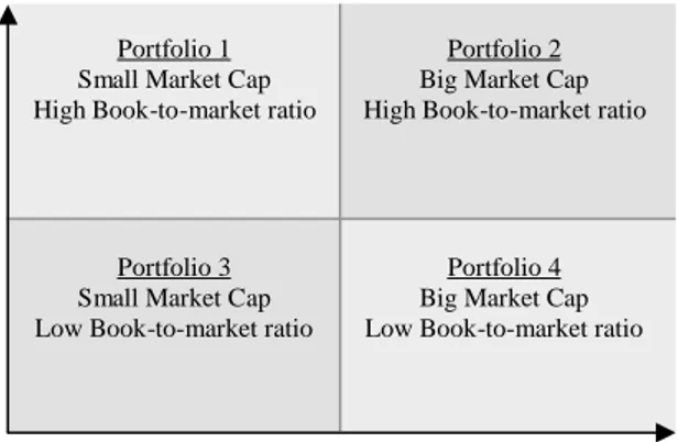
We sort our sample firms into two size categories (Big and Small, where the median market value is the criterion for dividing into Small and Big) and two book-to-market equity ratio categories (BE/ME low and BE/ME high), where again the median value is the dividing criterion. At the end of March each year, firms are allocated to the two size groups. Firms in each size group are allocated to the two book-to-market groups. Note that the ranking of size and book-to-market ratio values are done independently. From these four categories we define four portfolios, which will constitute our dependent variables.
Figure 4.1 The four portfolios defining the dependent variables
Size (Market Capitalization) BE/ME Ratio Small Big Low High Portfolio 1 Small Market Cap High Book-to-market ratio
Portfolio 3 Small Market Cap Low Book-to-market ratio
Portfolio 2 Big Market Cap High Book-to-market ratio
Portfolio 4 Big Market Cap Low Book-to-market ratio
13
Each portfolio will correspond to a different regression equation. We measure the return every month for the following portfolios.
• Small market value and High book-to-market ratio • Small market value and Low book-to-market ratio • Big market value and High book-to-market ratio • Big market value and Low book-to-market ratio
The number of firms vary between the portfolios and by year. The reason for this is the requirement that all necessary information regarding market value, P/E ratio and book-to-market ratio have to be available to be part of the study. Table 4.1 shows the number of firms in each portfolio each year.
Table 4.1 Number of firms in the different dependent variable portfolios 2012 2013 2014 2015 2016 SH 19 33 33 37 47 SL 13 25 28 29 32 BH 31 33 35 36 38 BL 31 35 38 45 52 Total 94 126 134 147 169
The dependent variable (Ri – Rf) will be the average of the returns of the firms in the cell that corresponds to one of the four portfolios/equations and is defined by the combination of size and book-to-market ratio in a 2 × 2 matrix. The reason for this is to attempt to neutralize surprising effects, which sometimes, in a very tangible way, affects the stocks’ return. Since we cannot observe the required return for a stock or a portfolio, we have to look at historical values for approximation. That approximation will mirror the expected return better if the surprise effects are neutralized. Of course, the implicit assumption is that the surprise effects in a portfolio on average is zero.
The specification of the different equations corresponding to the four cells in the matrix is designed to make it possible to isolate firms of different character in order to be able to analyze how different types of firms are correlated to the independent variables (Ri – Rf) , SMB and HML. More importantly however is that such a procedure makes it possible to differentiate the two variables that are hypothesized to increase the required return, namely small size and low book-to-market ratio, and analyze them separately. For example, it is expected that firms that are assigned to the smallest size and lowest book-to-market ratio may increase the return, but that the book-to-market ratio does not have any explanatory power for the combination Big firm-High book-to-market ratio.
14
For the four dependent variables, we have 60 observations. Even if we use the average return for the portfolio’s stocks, we will get such an average return each month, i.e. altogether 60 observations.
4.3 Independent variables
In order to define the explanatory variables in accordance with what Fama-French suggested (1992, 1993 and 1995), different portfolios were constructed.
All firms in the sample are sorted on the basis of size and book-to-market ratio. This is done independently of each other. It is important to recognize that it is not the returns associated with size and book-to-market in absolute numbers that are used as explanatory variables in the models where these variables are used. Instead, in the 1992 article, Fama-French shows how much bigger the return is for stocks in small companies compared to stocks in big companies and how much bigger the returns are for stocks with high book-to-market ratio compared to stocks with low book-to-market ratio.
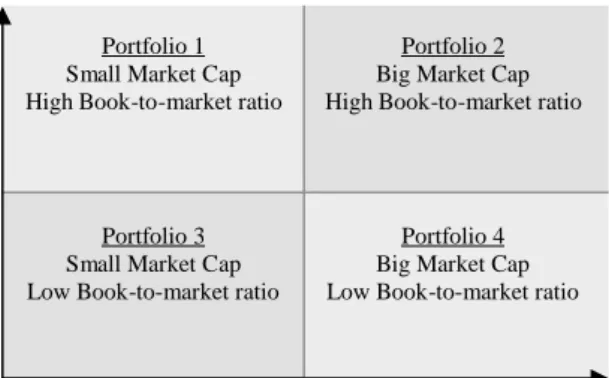
4.3.1 Size – Explanatory variable is designed as Small Minus Big (SMB)
We will measure size as market value on April 1 every year. From that we will construct two categories: Big and Small. We will use the median to classify the sample stocks either as Big or Small and create one portfolio from Big stocks and another one for Small stocks. Note that since the ranking of size and Book-to-market ratio values are done independently of each other, it means that all firms will end up in cells where the returns are defined by size and book-to-market ratio. From the two size categories and the two book-to-market categories, four portfolios are constructed in total, one for each combination of size and book-to-market. Figure 4.1 shows the resulting matrix
Figure 4.1 Construction of the SMB explanatory variable
Size (Market Capitalization) BE/ME Ratio Small Big Low High Portfolio 1 Small Market Cap High Book-to-market ratio
Portfolio 3 Small Market Cap Low Book-to-market ratio
Portfolio 2 Big Market Cap High Book-to-market ratio
Portfolio 4 Big Market Cap Low Book-to-market ratio
15
Again, for each of the four portfolios, the returns are observed on a monthly basis. In accordance with the Fama-French approach, the values of the returns in these cells will be used to define an explanatory variable for size as SMB (Small minus Big). The variable is constructed as the average return for the two portfolios containing Big firms. This number is then subtracted from the average return from the two portfolios containing Small firms. The formula used will therefore be:
Equation 4.1 𝑆𝑀𝐵 =1 2(𝑅𝑆𝑚𝑎𝑙𝑙𝐿𝑜𝑤+ 𝑅𝑆𝑚𝑎𝑙𝑙𝐻𝑖𝑔ℎ) − 1 2(𝑅𝐵𝑖𝑔𝐿𝑜𝑤 + 𝑅𝐵𝑖𝑔𝐻𝑖𝑔ℎ) 4.3.2 Book-to-market ratio (HML)
In a similar way we will define HML (High minus Low) by taking the average return on portfolios with a Low book-to-market ratio and subtract it from the average return of portfolios with a High market ratio. In accordance with the Fama-French study, we use two categories for book-to-market ratio: High and Low. The book-to-book-to-market ratio is dated January 1 for the studied year. Accordingly, we will get the value of HMLby using the following formula:
Equation 4.2 𝐻𝑀𝐿 =1
2(𝑅𝑆𝑚𝑎𝑙𝑙𝐻𝑖𝑔ℎ+ 𝑅𝐵𝑖𝑔𝐻𝑖𝑔ℎ) − 1
2(𝑅𝑆𝑚𝑎𝑙𝑙𝐿𝑜𝑤+ 𝑅𝐵𝑖𝑔𝐿𝑜𝑤)
In summary, we create two factors: SMB and HML, which show “difference in returns” between Small and Big firms and firms with a High book-to-market ratio and a Low book-to-market ratio. The value of SMB and HML are measured every month for the five years (2012-2016) from the end of April, 2012 to end of March 2016, which results in 60 observations for each factor. These are the observations that are used in the regressions where SMB and HML are explanatory variables.
4.3.3 P/E ratio (LMH)
Both Price and Earnings are dated January 1 for the studied year. Two groups based on the P/E ratio are constructed first. We use the median to classify the firms in two groups - Low P/E and High P/E. We then define LMH by subtracting the average return on the portfolio containing 𝑅𝐻𝑖𝑔ℎ𝑃/𝐸 from the portfolio containing 𝑅𝐿𝑜𝑤𝑃/𝐸:
Equation 4.3 𝐿𝑀𝐻 = 𝑅𝐿𝑜𝑤𝑃/𝐸− 𝑅𝐻𝑖𝑔ℎ𝑃/𝐸
16
There are some pitfalls to be aware of when using the P/E ratio. The market value is given by the market, but the earning per share is computed by the company’s accounting department and can be changed by some arbitrary rules. Involved here can be the use of historical costs in depreciation and inventory valuation, and in times with high inflation rates, historic cost depreciation will underrepresent true economic values since the replacement costs increase during time of high inflation. In general, P/E ratios have been inversely related to inflation, reflecting that earnings are of “lower quality” during times with high inflation. Another example is that during especially good years, profits can be transferred to tax allocation reserves.
It is also observed that P/E ratios vary across industries. Industries such as business software and biotechnology have the highest P/E ratios and also high growth rates. On the other hand, firms such as aero-space and manufacturing are in more mature or less profitable industries with limited growth have low P/E ratios. The relationship between growth and P/E is not perfect, but generally the P/E ratios appear to mirror growth opportunities.
When using P/E ratios, analysts have to be careful. It is impossible to say that a P/E ratio is too high or too low without referring to a company’s long-run growth prospects, as well as to the current earnings per share, relative to the long-run trend. An investor may very well pay a higher price per krona of current earnings if the investor expects the earning stream to grow more rapidly.
4.4 Market return
Market returns is approximated by OMX Stockholm Price Index (OMXSPI) which expresses the value of all stocks on the Stockholm Stock Exchange. OMXSPI mirrors only the market prices and is not adjusted for dividends.
4.5 Risk-free return
The risk-free return is based upon the interest on treasury bills with a maturity of three months. Since the interest rate on treasury bills is expressed on a yearly basis, we have to use the following formula to get the monthly rate:
Equation 4.4 𝑅𝑓(𝑡)= (1 + 𝑅´𝑓(𝑡))(12)1 − 1
17
In summary, four different portfolios have been designed with different combinations of size and book-to-market ratios. The return of these four portfolios will, together with the risk-free interest, define the dependent variable in different models, where depending on what model is analyzed, different combinations of the portfolios of SMB, HML, (𝑅𝑚− 𝑅𝑓) and LMH are used as independent variables.
4.6 Descriptive statistics
The independent variables used in our study, i.e. market risk premium, the two Fama-French variables SMB and HML, as well as the Price/Earning ratio (LMH), have been calculated each month for five years. That means 60 calculated observations on each variable during five years. Table 4.1 shows descriptive information about the variables.
Table 4.1 Descriptive information
Rm-Rf HML LMH SMB Mean 0.009278 -0.002341 0.001545 0.011445 Median 0.016165 -0.003178 0.001806 0.009258 Maximum 0.080226 0.041982 0.049059 0.065500 Minimum -0.099712 -0.052842 -0.029477 -0.039337 Std. Dev 0.037624 0.018169 0.015435 0.023144 Observations 60 60 60 60
The mean for both SMB and LMH are positive, which indicates that on average over the period small companies and companies with low P/E ratio have a bigger return than big companies and companies with high P/E ratios. At the same time, it indicates that companies with low book-to-market ratio will generate bigger return.
One of the conditions that has to hold in a regression analysis to be able to say something about the significance of the independent variables is that the error term has constant variance. If this is not the case, we are faced with the problem of heteroscedasticity, which will affect the standard deviation of the estimated coefficients. Breusch-Pagan-Godfrey tests and the White tests showed that our models fulfill the assumption of equal variance assumption (homoscedasticity).
18
Another factor that might influence the interpretation of our results is the presence of multicollinearity, which happens when the independent variables are correlated. To reduce the correlation between size and book-to-market value, Fama-French created two independent sortings of the sample. By constructing the variables this way, Fama-French was able to define the size effect to the SMB variable and the book-to-market effect to the HML variable. The LMH variable was constructed with a single sorting of the firms in terms of P/E-values. This was done to be able to investigate whether LMH mirrored the same risk factors as SMB and HML.
As can be seen in the table 4.2, no correlation is above 0.5. Therefore we do not have to be concerned with multicollinearity.
Table 4.2 shows the correlation between the independent variables. Rm-Rf SMB HML LMH
Rm-Rf 1.000000
SMB 0.031963 1.000000
HML 0.021229 -0.347822 1.000000
LMH 0.031097 0.313223 0.254777 1.000000
4.6 Specifications of models that are estimated
Since we want to analyse how well different models explain the return on the Stockholm Stock Exchange during the five-year period 2012-2016, we decided to use the CAPM as a reference point.
Equation 4.5 𝐸(𝑅𝑖𝑡) − 𝑅𝑓𝑡 = 𝛼𝑖+ 𝛽𝑖𝑡[𝐸(𝑅𝑚𝑡) − 𝑅𝑓𝑡]
In a second model, we use Fama and French’s criticism of the CAPM. Extensive previous empirical work convinced us that there are two firm characteristics, in addition to the beta-coefficient, that improve the explanation of the return of a stock, namely size and book-to-market ratio. Furthermore, Fama-French found that stocks of small companies and companies with a high book-to-market ratio give a better return than the average of the market. This is the background to our choice of the second model, which is a Fama-French three-factor model.
Equation 4.6 𝐸(𝑅𝑖𝑡) − 𝑅𝑓𝑡 = 𝛼𝑖 + 𝑏𝑖[𝐸(𝑅𝑚𝑡) − 𝑅𝑓𝑡] + 𝑠𝑖𝑆𝑀𝐵𝑡 + ℎ𝑖𝐻𝑀𝐿𝑡 + 𝜀𝑖𝑡
19
Thirdly, the Fama-French traditional three-factor model will be extended to a four-factor model by adding a LMH factor to study the effects of including a variable measuring the impact of the P/E ratio. The way we will perform the analysis is to see whether SMB and HML can be regarded as proxy variables for the Price/Earnings ratio. The hypothesis is that, if the coefficient for LMH is positive and significant at the same time as the values of the coefficients of SMB and HML will change as a result of the inclusion of HML, then we can say that P/E helps explain the return of the dependent variable, and SMB and HML are not to be regarded as proxies for LMH.
Equation 4.7
E(Rit)-Rft = αi+ βi[E(Rmt)-Rft] + siSMBt + hiHMLt + piLMHt+ εit
Where
Rit= Return on portfolio i at time t, where i =1...4 and indicates what dependent portfolio we will estimate and t = 1….60 months
Rmt = Market return at time t
Rft= Risk-free rate of return at time t
SMBt= Size factor for time t (Small minus Big) at time t HMLt= Book-to-market value (High minus Low) at time t LMHt= Price/Earning ratio (Low minus High) at time t
Equations 4.5 – 4.7 were estimated by ordinary least squares (OLS) by using return data for 60 months (2012-2016), since we, through tests, could assume homoscedasticity and the absence of multicollinearity. Furthermore, our models are linear in the parameters.
5. Results and Analysis
The results from the ordinary least squares (OLS) time-series regression for the three models are presented below.
5.1 CAPM
In the first set of equations we examine the explanatory power of the CAPM on four independently created portfolios. An OLS time-series regression analysis has been performed on equation 4.5.
20
Table 5.1 shows the intercept and the coefficients for the market risk premium (Rm-Rf) and the explanatory power of the regressions, measured by adjusted R̅2.
Table 5.1 Results for CAPM
CAPM R̅2 SL 0.018331 (4.085001**) 0.957467 (8.203275**) 0.529106 SH 0.012392 (3.609748**) 0.983637 (11.01572**) 0.671027 BL 0.003567 (1.809361) 0.953725 (18.60123**) 0.853962 BH 0.004632 (2.827872**) 0.948058 (22.25257**) 0.893343
The t-test is shown in parenthesis for every variable *Significant at five percent level
**Significant at one percent level
The value of the intercept shows how well the calculated value of return compares to the real value. The intercept is positive and significant at the 1-percent level, indicating that the model will underestimate the return of the portfolio. This is the case for all portfolios except the BL portfolio (consisting of big companies with a low book-to-market value). The coefficient for the market risk premium (β) is significant at the 1-percent level for all portfolios. We also see that the CAPM produces adjusted 𝑅̅2 that varies greatly between the portfolios – from 53% for the SL portfolio to
89% for the BH portfolio.
The beta values are similar for all portfolios. If the return of asset i exactly mirrors the risk of the portfolio m, then 𝛽 = 1. If the returns are completely unrelated to each other, then 𝛽 = 𝐶. If 𝛽 > 1, it means that the asset is a volatile asset. If 𝛽 < 1, it means that it is a defensive asset. The beta values vary between 0,95 and 0,98, i.e. close to unity, indicating that the return of the portfolios vary in tune with the market, marginally on the defensive side.
5.2 Fama-French three-factor model
The Fama-French three-factor model (1993) was created to include the relation between average return and size (market capitalization) together with the relation between average return and book-to-market ratios. SMB (Small Minus Big) is used to capture size risk and HML (High Minus Low) to
21
capture value risk. A positive SMB factor measures higher returns for small stocks (small capitalization) compared to big stocks (large capitalization). Value stocks are characterized by high book-to-market ratio and growth stocks are characterized by low book-to-market ratio. A positive HML factor represents a higher return for value stocks compared to growth stocks. When Fama-French published their study in 1993, these were the two well-known patterns in average returns that were left unexplained by CAPM. For each of the four independently created portfolios, an OLS time-series regression analysis has been performed on equation 4.6:
E(Rit)-Rft = αi+ bi[E(Rmt)-Rft] + siSMBt + hiHMLt + εit
The results are shown in table 5.2 showing the intercept and the coefficients for market risk premium, market size, book-to-market ratio, and adjusted 𝑅̅2.
Table 5.2 Results for Fama-French three-factor model FF3 SMB HML R̅2 SL 0.005033 (2.865909**) 0.945672 (22.91781**) 1.010384 (14.12458**) -0.787202 (-8.6417**) 0.941275 SH 0.002547 (1.301765) 0.957462 (20.82864**) 1.008237 (12.65198**) 0.619621 (6.10587**) 0.913009 BL 0.002547 (1.301765) 0.957462 (20.82864**) 0.008237 (0.103367) -0.380379 (-3.7483**) 0.882872 BH 0.005033 (2.865909**) 0.945672 (22.91781**) 0.010384 (0.145160) 0.212798 (2.336050*) 0.900172
The t-test is shown in parenthesis for every variable *Significant at five percent level
**Significant at one percent level
When we introduce the Fama-French variables of size and the book-to-market ratios, the estimated coefficients will change as well as the adjusted 𝑅̅2 as shown in table 5.2. If the exposures to the three
factors, 𝛽𝑖, 𝑠𝑖, and ℎ𝑖 capture all variation in expected returns, the intercept in equation 4 is zero for all securities and portfolios i. They are significantly different from zero for the SL and BH portfolio. Two things happen with adjusted 𝑅̅2. First the values are higher than for the CAPM – ranging from
88 % to 94 %, compared to 53% to 89 % for CAPM. Furthermore, comparing the different portfolios, we see that for portfolio SL, the Fama-French model has a much better (almost double) explanatory power than the CAPM. Also, SH shows a big difference in explanatory power, while for both BH and BL, the differences between CAPM and FF3 are just a couple percent. The Fama-French traditional
22
three-factor model is, to a high extent, able to explain the variation in returns for the investigated portfolios, and functions quite well in the Swedish stock market.
The coefficient of the market risk premium is significant at the 1-percent level for all portfolios and has approximately the same value compared to the CAPM for the BL and the BH portfolio and a marginal reduction for SL and SH. The values for all four portfolios are close to 1, indicating that the portfolio firms follow the general market, which means that the risks associated with the different portfolios mirror the risk of the market portfolio. This is expected since the sample consists of stocks from OMX Large Cap and OMX Mid Cap.
The coefficients for Market premium and HML are significant at a 1-percent level for all portfolios except for the BH portfolio, which is significant at the 5-percent level. For the HML, the coefficients change from being positive and significant for companies with a high book-to-market ratio to negative and significant for companies with a low book-to-market ratio. In SH and BH, the value stocks generate a positive value of HML, which means a higher return for value stocks compared to growth stocks, while the parameter value of HML in SL and BL shows that in those cells, there is a higher return for growth stocks compared to value stocks. This led us to conclude that the returns with high book-to-market ratios require a risk premium, while that premium is reduced for companies with low book-to-market ratios.
The SMB coefficients are significant for the small companies (SL and SH), but insignificant for the big companies. There is a direction for the SMB coefficient. It goes from being positive and significant for small companies to be insignificant for big companies. This would indicate that the returns in portfolios with small companies require a risk premium, while the required return for big companies are reduced.
Furthermore, it can be observed that the portfolios that, under SMB, are allotted to the category of Small market value (SL, SH), show a big difference between the adjusted 𝑅̅2 comparing CAPM and
the Fama-French three-factor model, while the portfolios that, under SMB, are allotted to Big market value do not differ very much.
5.3 Adding LMH to Fama-French three-factor model
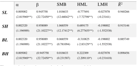
For each of the four independently created portfolios, an OLS time-series regression analysis has been performed on equation 4.7. The results are shown in table 5.3
23
Table 5.3 Result Fama-French three-factor model with the addition of LMH FF4 SMB HML LMH 𝑅̅2 SL 0.005002 (2.815969**) 0.945758 (22.72450**) 1.018633 (12.66042**) -0.777691 (-7.72798**) -0.027078 (-0.23161) 0.940266 SH 0.002320 (1.196989) 0.958089 (21.10227**) 1.068559 (12.17412**) 0.689175 (6.277655**) -0.198002 (-1.552538) 0.915146 BL 0.002320 (1.196989) 0.958089 (21.10227**) 0.068559 (0.781094) -0.310825 (-2.83129**) -0.198002 (-1.552538) 0.885749 BH 0.005002 (2.815969**) (0.945758 (22.72450**) 0.018633 (0.231587) 0.222309 (2.209110*) -0.027078 (-0.231618) 0.898456
The t-test is shown in parenthesis for every variable *Significant at five percent level
**Significant at one percent level
The Fama-French three-factor model was extended to a four-factor model by adding LMH as a way of incorporating the P/E ratio. The risks implicit in the P/E ratios are assumed to be related to exaggerated expectations about the future growth of earnings and dividends. The implication is that exaggerated optimism results in high P/E ratios, and exaggerated pessimism regarding earnings and dividends results in stocks with low P/E (Basu 1977 and 1983).
The results are shown in table 5.3. The LMH variable adds very little or decreases the explanatory power of the return for the different portfolios. The intercept does not change when the LMH variable is added. The hypothesis is that if HML and SMB are acting as proxies for risks associated with LMH, then we would expect the coefficients for HML and SMB to change when LMH is introduced. The negative values of the coefficients decrease for the HML variable and the variable is still significant at the 1-precent level. The coefficient of the LMH variable is negative but insignificant. The values of the SMB coefficient for the SL and SH increase and are significant at the 1-percent level. One conclusion is that the addition of LMH results in an increase of the value of the coefficients in all portfolios. Looking at the results, we conclude that SMB and HML do not act as proxies for the risk associated with the P/E values, and since the coefficients for the LMH variable is insignificant, we conclude that the P/E ratio as such is not influencing the expected returns.
24
One important implication of any asset valuation model is that, ceteris paribus, riskier stocks will have lower P/E ratios. This can be explained by using the dividend discount model, which has a formula that states that the intrinsic value of a stock is the present value of all future cash payments including dividends and sale price from ultimate sale. These flows are discounted at the appropriate risk adjusted interest rate.
For any expected cash flows, the present value of those flows will be lower when the stream is riskier, since riskier stocks will use a higher discount rate in the evaluation model. Hence, the stock price of the ratio of price to earnings will be lower and therefore, the P/E ratio must be lower. Thus, if pricing is efficient, the stock with a lower price must be associated with higher risk.
One can find small, risky stocks with high P/E ratios. This does not contradict the claim that P/E ratios should fall with risk. It is only a result of the market expecting high growth rates of those companies. This is the implication of the ceteris paribus condition we wrote as a condition for our statement, i.e. given a growth prediction, the P/E ratio will be lower when the risk is higher.
6. Conclusions
The purpose of the study is to investigate empirically how well three different pricing models explain average excess returns on the portfolios defined in figure 4.1, using time series data during 2012-2016, which has not been analyzed before.
The asset-pricing model (CAPM) of Sharpe (1964), Litner (1965) and Mossin (1966) has influenced how both academicians and practitioners look upon the relationship between average return and risk for a long time. We started our analysis by using the original CAPM model, based upon the efficient market hypothesis suggesting that at any given time, prices fully reflect all available information on a particular stock and that the market represents the best estimate of intrinsic value. It implies that that the expected returns of a security are a positive linear function of the market betas and that the market betas are sufficient to describe the cross-section of expected returns. We analyzed the original CAPM model’s ability to explain the average return on stocks on the Stockholm Stock Exchange during 2012-2016. Over time, the original CAPM has been contradicted by many researchers, starting from Banz (1981), who found that market equity adds to the explanation of the cross-section of average returns resulting from market betas. Basu (1983) found that earnings/price ratio helps explain the cross-section of average returns on US stocks.
25
A large number of studies have been performed within this field. One solid conclusion from those studies is that if assets are priced rationally, then the stock risks are multidimensional, implying that there are patterns in average returns related to market value and book-to-market ratio (The Royal Swedish Academy of Sciences, 2013; Fama-French 2015). We therefore looked at how a three-factor Fama-French model including market value and book-to-market ratio would perform compared to the CAPM.
We found that the Fama-French three-factor model directed at capturing the size (market value) and book-to-market ratio functions quite well for the Swedish stock market during 2012-2016 and performs much better, measured by adjusted 𝑅̅2 (Adjusted 𝑅̅2 ranging from 88% to 94%), than the
CAPM (Adjusted 𝑅̅2 ranging from 53 to 89%) in explaining average returns on portfolios formed to
produce large spreads in size and book-to-market ratios. Similar results were obtained by Hjalmarsson and Pantzar (2012), who used data for 2002-2012.
Since Price/Earning or its inverse earning/price have been suggested to represent possible anomalies, we added a fourth factor – Price/Earning in the form of LMH – to the three-factor model. We analyzed whether the addition of the Price/Earning variable would increase the explanatory power of the average returns of the different dependent variables portfolios. The analysis showed that the HML and SMB variables did not act as proxies for LMH and therefore we concluded that the P/E ratio as such is not influencing the expected returns in the sample we examined.
Based on the evidence presented in this study, we conclude that the Fama-French three-factor model gives the best description of average returns on the portfolios investigated.
6.1 Future research
When we developed the three-factor model we did not consider alternative definitions of SMB and HML. We followed the Fama-French design of the 2 × 2 sort on size and book-to-market ratio. This choice is however arbitrary. In the future, it would be illuminating to test the sensitivity of asset pricing result to other choices.
We believe that the specification of different equations directed at capturing different patterns in average stock returns is a way to improve the explanation of average excess returns. Our suggestion
26
would be to test the results of adding profitability and investment patterns as explanatory variables, as suggested by Novy-Marx (2012) and Fama-French (2015).
Other extensions could be to check different time periods, and if the result would differ between Large Cap, Mid Cap, and Small Cap, and also between different industries, on the Stockholm Stock Exchange.
27
References
Allergren, C. F. and Wendelius, K. A. (2007). “CAPM – i tid och otid,” Bachelor thesis Handelshögskolan vid Umeå universitet
Banz, R.W. (1981), “The relationship between return and market value of common stocks,” Journal of Financial Economics 9, 3-13.
Basu, S. (1977), “Investment performance of common stocks in relation to their price- earnings ratios: A test of the efficient markets hypothesis,” Journal of Finance 32, 663-682.
Basu, S. (1983), “The relationship between earnings yield, market value, and return for NYSE common stocks: Further evidence,” Journal of Financial Economics 12, 129-156.
Belani, N and Jabbari, S (2007). “P/E-tal som investeringsstrategi”, Department of Economics, Uppsala University.
Booson, A and Swahn, L (2015). “Popularitet på aktiemarknaden.”. Department of management and Engineering, Linköping University.
Bodie, Z., Kane, A. and Marcus, A. (2014), “Investments,” 10th Global Edition, McGraw-Hill
Burton, E. and Shah, S. (2013). Behavioral finance. Hoboken: Wiley.
Ergul, E and Johannesson (2009), “Famas och Frenchs två faktorer: proxyvariabler för konkursrisk?” Stockholm School of Economics.
Fama, E.F. (1965), “The behavior of stock market prices,” Journal of Business 38, 34-105.
Fama, E.F. (1970), “Efficient capital markets: a review of theory and empirical work”, Journal of Finance 25, 383-417.
Fama, E.F. and K.R. French (1992), “The cross-section of expected stock returns,” Journal of Finance 47, 427-466.
28
Fama, E.F. and K.R. French (1992), “Common risk factors in the returns on stocks and bonds” Journal of Financial Economics, 33, 3-36.
Fama, E.F. and K.R. French (1995), “Size and Book-to-Market factors in earnings and returns, The journal of Finance, Vol. 50 No.1, 131-155.
Fama, E.F. and K.R. French (2015), “Five factor Asset Pricing Model”, Journal of Finance Economics, Vol. 116(1), 1-22
Fama, E.F. and J.D. MacBeth (1973), “Risk, return and equilibrium: empirical tests,” Journal of Political Economy 81, 607-636.
Fransson Johnsson, D. Lööf, H. Rodell, K and Ryd, M. (2007). “Överavkastning vid återköp av aktier,” Department of Business Administration, Lund University.
Fryklund, H. and Mlinaric, R. (2016). “Efficient market hypothesis: testing for price predictability on the OMX Stockholm 30 Index,”. Bachelor Thesis. University of Gothenburg.
Gujarati, D. and Porter, D. (n.d.). Basic econometrics. 5th ed. Boston: McGraw-Hill.
Hjalmarsson, L. and Pantzar, J. (2012), “Capital Asset Pricing Model and Fama-French trefaktormodell”. Chalmers University of Technology, Gothenburg.
Jensen, M.C. (1968), “The performance of mutual funds in the period 1945-1964”,Journal of Finance 23(2), 389-416.
Kahneman, D. and A. Tversky (1984), “Choices values and frames,” American Psychologist 39, 341-350.
29
Hjalmarsson, L and Pantzar, J (2012). “Capital Asset Pricing model och Fama-French trefaktor-modell”, Chalmers University of Technology, Gothenburg.
Lintner, J. (1965), “The valuation of risk assets and the selection of risky investments in stock portfolios and capital budgets,” Review of Economics and Statistics 47, 13-37.
Markowitz, H. (1959), Portfolio Selection: Efficient Diversification of Investments, Yale University Press.
Mossin, J. (1966), “Equilibrium in a capital asset market,” Econometrica 34(4), 768-783.
Nicholson, F. (1960), “Price-Earnings Ratios” Financial Analysts Journal, Vol 16, No 4, 43-45.
Nicholson, F. (1968), Price Ratios in relation to investment results”, Financial Analysts Journal, Vol 24, No 1, 105-109.
Novy-Marx, R. (2013), ”The other side of value: The gross profitability premium”. Journal of Financial Economics Vol 108, No 1; 1-28.
Pettersen, A. (2011). “An investment strategy based on P/E ratios,” Lund School of Economics and Management, Lund University.
Rehnby, N. (2016) “Does the Fama-French three –factor model and Carhart four-factor model explain portfolio returns better than CAPM?”. Karlstad Business School, Karlstad University.
Samuelson, P.A. (1965), “Proof that properly anticipated prices fluctuate randomly,” Industrial Management Review 6, 41-49.
Sharpe, W.F. (1964), “Capital asset prices: A theory of market equilibrium under conditions of risk,” Journal of Finance 19(3), 425-442.
Shiller, R.J. (1981), “Do stock prices move too much to be justified by subsequent changes in dividends?” American Economic Review 71, 421-436.
30
Shiller, R.J. (1984), “Stock prices and social dynamics,” Carnegie Rochester Conference Series on Public Policy, 457-510.
The Royal Swedish Academy of Sciences (2013). “Understanding asset prices”. Scientific background on the Sveriges Riksbank Prize in Economic Sciences in memory of Alfred Nobel 2013.