One General Approach For Analysing Compositional Structure Of Terms In Biomedical Field

One General Approach For Analysing

Compositional Structure Of Terms In

Biomedical Field

Yang Chao

Peng Zhang

MASTER THESIS 2012

Postadress: Besöksadress: Telefon:

Box 1026 Gjuterigatan 5 036-10 10 00 (vx)

551 11 Jönköping

One General Approach For Analysing

Compositional Structure Of Terms In

Biomedical Field

Yang Chao

Peng Zhang

Detta examensarbete är utfört vid Tekniska Högskolan i Jönköping inom ämnesområdet informatik. Arbetet är ett led i masterutbildningen med inriktning informationsteknik och management. Författarna svarar själva för framförda åsikter, slutsatser och resultat.

Handledare: He Tan

Examinator: Vladimir Trasov Omfattning: 30 hp (D-nivå) Datum: 24 March 2013 Arkiveringsnummer:

I

Abstract

The root is the primary lexical unit of Ontological terms, which carries the most significant aspects of semantic content and cannot be reduced into small constituents. It is the key of ontological term structure. After the identification of root, we can easily get the meaning of terms. According to the meaning, it’s helpful to identify the other parts of terms, such as the relation, definition and so on. We have generated a general classification model to identify the roots of terms in this master thesis. There are four features defined in our classification model: the Token, the POS, the Length and the Position. Implementation is followed using Java and algorithm is followed using Naïve Bayes. We implemented and evaluated the classification model using Gene Ontology (GO). The evaluation results showed that our framework and model were effective.

II

Acknowledgements

We would like to thank our supervisor, Dr. He Tan who supported perfectly during this master thesis work with her wise advices and guidance and also our examiner, Dr. Vladimir Tarasov for his useful advices and discussions on our thesis work.

Yang Chao Peng Zhang

III

Key words

Key words: Gene ontology, Machine learning, Classification, Bayes

IV

Contents

2.2.3 Features of the Classification Model ... 10

3 Research Methods ... 13

3.1 Awareness of the Problem: Literature Search ... 14

3.2 Suggestion ... 15

3.3 Development ... 15

3.4 Evaluation: Cross-validation ... 16

3.5 Conclusion Phase ... 17

4 Framework and practical methods ... 18

4.1 Framework of supervised machine learning method ... 18

4.2 The development of system ... 21

4.2.1 Identification of required data and collecting the dataset ... 21

4.2.2 Data preparation and data processing ... 21

4.2.3 Algorithm selection and training ... 25

4.2.4 Evaluation with test set ... 27

4.2.5 Implementation ... 27

5 Results ... 28

5.1 Practical Results ... 28

6 Analysis and discussion ... 34

6.1 Analysis the results based on the method for extracting the features ... 34

6.2 Analysis the results based on the size of training data set ... 35

6.3 Analyse the results based on the final test data result ... 36

7 Conclusion and Future work ... 38

8 References ... 39

9 Appendix ... 43

9.1 The part of training data set’s POS evaluation results, the italic means the tokens were marked wrong ... 43

V

List of Figures

Equation 2-1: The equation for conditional assumption………8

Equation 2-2: The fundamental equation for the Naïve Bayes classifier...9

Equation 2-3: The formula for target value Y……….9

Equation 2-4: The formula of Naïve Bayes probability model……….9

Equation 2-5: The laplace smoothing……….10

Equation 4-5: The target formula is based on Naïve Bayes algorithm…25

Equation 5-5: The accuracy calculation formula……….31

Table 2-6: The POS tagging………..12

Table 4-3: The numbers of different lengths of terms………...21

Table 4-4: The features of the training set……….24

Table 5-9: The accuracy of 9 sets of test dataset………33

Table 6-2: The test data set result with training data with 200 terms…..36

Table 6-3: The terms marked wrong in three ways………37

Figure 4-1: The process of supervised ML……….18

Figure 4-2: The classification model……….19

Figure 5-1: Extract the dataset 1……….29

Figure 5-2: Extract the dataset 2……….29

Figure 5-3: Extract the dataset 1 with features………30

Figure 5-4: Extract the dataset 2 with features………...30

Figure 5-6: The training dataset with classified………..32

Figure 5-7: The test dataset 1 with probability………32

Figure 5-8: The final test dataset 1 without possibility………..33

VI

List of Abbreviations

ML: Machine Learning TM: Text Mining

SRL: Semantic Role Labeling POS: Part Of Speech

SGD: Saccharomyces Genome Database MGI: Mouse Genome Informatics SML: Supervised Machine Learning NN: Noun JJ: Adjective NNS: Plural VB: Verb RB: Adverb IN: Preposition

1

1 Introduction

Ontology links concept labels to their interpretations, specifications of their meanings including concepts definitions and relations to other concepts. Apart from relations such as is-a, generally presented in almost any domain, ontologies also model domain-specific relations, e.g. has-location specific for the biomedical domain. Therefore, ontologies reflect the structure of the domain and constrain the potential interpretations of terms [1].

A term is defined as a textual realization of a specialized concept. Text definitions precisely state the exact meaning of a term. Not all terms have text definitions. Text definitions are interpreted by users, not computers. It has been noted that many term names are compositional, and indicate implicit relationships to terms. The existence of composite terms leads to redundancy in both text definitions and relationships [2]. The redundancy means that the compositional nature of many terms leads to an increase in the number of relationships and consequent increase in complexity of the ontology. Effective term parsing will reduce the redundancy in biomedical ontologies [3].

The term parsing not only can reduce the redundancy, but also can used for text mining applications such as Semantic Role Labeling (SRL) system.

The sentence-level semantic analysis of text is concerned with the characterization of events, such as determining “who” did “what” to “whom”, “where”, “when” and “how”. It plays a key role in TM applications such as Information Extraction, Question Answering and Document Summarization [4]. The predicate of a clause expresses “what” took place, and other sentence constituents express the participants in the event. SRL is a process that, for each predicate in a sentence, indicates what semantic relations hold among the predicate and its associated sentence constituents [5]. However the development of SRL systems for the biomedical domain is frustrated by the lack of large domain specific corpora that are labeled with semantic roles.

Researchers found that ontological concepts typically are associated with textual realization which is to give precise meaning of concepts within context of a particular ontology in many cases [6]. Intuitively, ontological concepts, relations,

2

rules and their associated textual definitions can be used as the frame-semantic descriptions imposed on a corpus. Our supervisor has proposed one method for building corpus which is labeled by semantic role labeling for the biomedical domain. The method makes use of domain knowledge provided by ontology [7]. By this method, a corpus has been built which is related to transport events. In order to extend the corpus and get the ontological concepts, relations, rules and their associated textual defintions not just based on the transport events, we intend to develop a general method that supports parsing and visualizing lexical properties of ontological terms.

As an important step towards fulfilling the objective, formulating correct research questions has a vital role. We have mentioned the research question as followed in next section.

1.1 Purpose/Objectives

In this master thesis, we will do the first step for analyzing the compositional structure by identifying the roots of terms, because the root is the key of the term structure. After the identification of root, we can easily get the meaning of terms. According to the meaning of terms, it’s helpful to identify other parts such as relations, rules and so on. The purpose of this thesis work is formulated in two questions:

1. What is the method for identify the roots of terms?

2. What general theory framework is needed regarding support of the method classification we chosen?

1.2 Background

We proposed a classification model for identify the roots of terms and defined four features: Token, Part of speech (POS), Length, Position. Token means different word in ontology terms. POS means linguistics category of words (such as noun, prep, adjective, etc.). Length means numbers of tokens in one term. Position means the position of tokens in each term. Based on this model, we used Gene Ontology (GO) data as implemented and evaluated.

3

1.3 Limitations

Our method has no limitation. It is a general classification model we developed. It is not only applied for biomedical field, but also for other filed ontologies such as the business filed and the industry field.

The scope of the project is that implemented in the GO.

1.4 Thesis outline

This document is structure as six chapters:

 Chapter 1 which has covered the outline of thesis is basically introduction part that presents ontology, text, term parsing, semantic role labeling, background and objective work.

 Chapter 2 gives the definitions for main concepts used in the implementation.

 Chapter 3 describes the research method followed for reaching the thesis goals.

 Chapter 4 deals with introducing framework as well as explaining the method used for implementation.

 Chapter 5 presents the results achieved during the thesis work.

4

2 Theoretical Background

This chapter will include the basic knowledge regarding the definition of ontology, especially GO and what is the supervised machine learning. It also includes the definition of classification and Naïve Bayes Algorithm, how they work as well as the basic knowledge of POS. The reader of this research could understand basic knowledge which is related to object of our thesis.

2.1 Ontology

In computer science, ontology formally represents knowledge as a set of concepts with a domain and the relationship between pairs of concepts. It can be used to model a domain and support reasoning about entities [8].

In the implementation, ontology is a detailed description of the conceptualization. The core role is to define the specialized vocabulary of a particular area or field, as well as the relationship between them. The basic concept of this series as the cornerstone of a building project provides a unified understanding for the exchanged parties. In support of these series concepts, knowledge of the search, the efficiency of the accumulation and sharing will be greatly improved, and in the true sense of the knowledge reuse and sharing become possible [9].

Ontology can be divided into four types: Domain ontology, General ontology, Application ontology and Representation ontology. Domain ontology contains the knowledge of the specific type of the field (such as electronics, machinery, medicine and teaching); General ontology is covered in a number of domain, often referred to as the core of the ontology; Application ontology contains all the knowledge required for a specific domain modeling; Representation ontology is not only confined to a specific area, but also provide the entity used to describe things, such as the frame ontology, which defines the framework, the concept of slot [10]. In this master thesis, we have used GO as the implemented data. It is a successful application in biomedical field.

2.1.1 Gene Ontology

In this master thesis, we have chosen GO as the data set in the evaluation because the GO is one of the most biggest and successful applications in biomedical field. It

5

covers different kinds of events in biology field. The events are carefully named in ontologies.

GO is made by GO consortium. GO consortium's intention is to create shared biological information resources, which can be able to allow the industry to take advantage of the public vocabulary and semantic description of gene products.

GO consortium was built in the early 1998. GO project is work alliances in the area of information integration. Two sides of work are 1) providing gene production’s consistency description in different databases, 2) classification and characteristics of standardization sequence [11].

The Gene Ontology project is a major bioinformatics initiative with the aim of standardizing the representation of gene and gene product attributes across species and databases. The project is provides a controlled vocabulary of terms for describing gene product characteristics and gene product annotation data from GO Consortium members, as well as tools to access and process this data.

The GO is a collection of three ontologies, which partitioned into orthogonal domain, contains molecular function, biological process and cellular component. The biological process covers different kinds of events. It operates or sets molecular events with a defined beginning and end, pertinent to the functioning of integrated living units: cells, tissues, organs and organisms. A biological process is series of events accomplished by one or more ordered assemblies of molecular functions. A biological process is not equivalent to a pathway; at present, GO does not try to represent the dynamics or dependencies that would be required to fully describe a pathway.

GO consists of terms that are defined as a textual of a specialized concept. Terms may also have one or more synonyms. Terms are interconnected via typed binary relationships, for example, ‘interleukin is a cytokine’ or ‘small ribosomal subunit part of mitochondrial ribosome’ [13]. The existence of composite terms leads to redundancy in both text definitions and relationships in GO [14]. For example, the term ‘cytokine’ has redundant definitions embedded in the text definitions for ‘cytokine metabolism ’and‘cytokine biosynthesis. The redundancy in relationships manifests itself as ‘cytokine metabolism’ and ‘cytokine biosynthesis’ being related

6

via “is-a” to both ‘protein metabolism’ and ‘protein biosynthesis’. Thus, the effective method for terms parsing is necessary.

For SRL systems in the biomedical domain, it lacks of large domain specific corpora that are labeled with semantic roles. Many biomedical text mining systems have mainly used ontologies as terminologies to recognize biomedical terms, by mapping terms occurring in text to concepts in ontologies, or used ontologies to guide and constrain analysis results, by populating ontologies. Our supervisor believes that ontological, as a structured and semantic representation of domain-specific knowledge, can instruct and ease all the tasks in corpus construction.

GO, one of the biggest ontologies in biomedical field, many concepts in GO that comprehensively describe a certain domain of interest in biomedical field. GO biological process ontology, containing 20,368 concepts, provides the structured knowledge of biological processes that are recognized series of events or molecular functions. The ontological terms can be seen as phrase that exhibit underlying compositional structures [41]. For example, for ‘protein transport’ in GO, if we have known the compositional structures of some direct subclasses describing various types of protein transport, we will easily to know what are the possible predicates evoking the protein transport events. Then we can use the classes and relations to define the semantic frame ‘Protein Transport’, decided the participants involved in the event, and listed the domain-specific words evoking the frame [41]. As such, domain knowledge provided by ontologies, such as GO biological process ontology and molecular function ontology will instruct us in building large frame corpora for the domain. An important step towards building large corpora is analyzing the compositional structure of terms. The GO covers different kinds of events related to Gene products. Hence, we used GO as our implemented data.

2.2 Machine Learning

Machine learning is one of the core research areas of artificial intelligence. The initial motivation is to let a computer system with a person's ability to learn in order to achieve artificial intelligence. It is well known that if the system does not have the ability to learn the system can hardly be considered to have intelligent. It is widely used in the definition of machine learning to "use the experience to improve the performance of the computer system itself" [15, 16].

7

Machine learning has different algorithm types. They are supervised learning, unsupervised learning, semi-supervised learning reinforcement learning, learning to learn. Supervise learning is the machine learning task of inferring a function from labeled training data. The training data consist of a set of training examples. In this master thesis, we want to generate a general method for analyzing the compositional structure of ontological terms. The task is to identify the root of terms. Our problem is a supervised learning problem. It is to classify each token to “Root” or “NoRoot”.

2.2.1 Classification

In machine learning and statistics, classification is the problem that identifies a new observation belongs to a set of predefined categories. It depends on the basis of a training set of data containing observations whose category membership is known [17]. The individual observations are analyzed into a set of quantifiable properties, known as various explanatory variables and features. An algorithm that implements classification, especially in a concrete implementation, is known as a classifier. The term "classifier" sometimes also refers to the mathematical function, implemented by a classification algorithm that maps input data to a category.

Terminology across fields is quite varied. In statistics, where classification is often done with logistic regression or a similar procedure, the properties of observations are termed explanatory variables and the categories to be predicted are known as outcomes, which are considered to be possible values of the dependent variable. In machine learning, the observations are often known as instances, the explanatory variables are termed features and the possible categories to be predicted are classes [17].

In this master thesis, classification means we may know for certain that there are so many classes, and the aim is to establish a rule whereby we can classify a new observation into one of the existing classes. It is considered as an instance of supervised learning. According to our classification model, when the new tokens arrive, we classify them into different two categories: one category is tokens are marked into root, the other is tokens are not marked into root.

2.2.2 Naïve Bayes

8

A naive Bayes classifier is a simple probabilistic classifier based on applying Bayes' theorem with strong independence assumptions. In probability theory, to say that two events are independent means that the occurrence of one does not affect the probability of the other. Similarly, two random variables are independent if the observed value of one does not affect the probability distribution of the other. An advantage of the naive Bayes classifier is that it only requires a small amount of training data to estimate the parameters necessary for classification [18].

Depending on the precise nature of the probability model, naive Bayes classifiers can be trained very efficiently in a supervised learning setting. In many practical applications, parameter estimation for Naive Bayes model uses the method of maximum likelihood; in other words, one can work with the naive Bayes model without believing in Bayesian probability or using any Bayesian methods [19]. The Naïve Bayes algorithm is a classification algorithm based on Bayes rule, that assumes the attributes X1…Xn are all conditionally independent of one another, given

Y. The value of this assumption is that it dramatically simplifies the representation of

P (X|Y), and the problem of estimating it from the training data. P (X|Y) means the

possibility that event X occurs with the condition B.

Consider, for example, the case where X=X1 or X=X2. In this case,

P(X|Y)=P(X1|X2,Y)P(X2|Y)=P(X1|Y)P(X2|Y). It follows above definition of

conditional independence. More generally, when X contains n attributes which are conditionally independent of one another given Y, we have



Equation 2-1: The equation for conditional assumption [19]

Now we derive the Naïve Bayes algorithm, assuming in general that Y is any discrete-valued variable, and the attributes X1…Xn are any discrete or real-valued attributes.

Our goal is to train a classifier that will output the probability distribution over possible values of Y, for each new instance X that we ask it to classify. The expression for the probability that Y will take on its possible value, according to Bayes rule, is

9







Equation 2-2: The fundamental equation for the Naïve Bayes classifier [19] As the equation 2-2 shown, given a new instance Xnew=(X1…Xn), this equation shows

how to calculate the probability that Y will take on any given value, given the observed attribute values of Xnew and given the distributions P(Y) and P(Xi|Y)

estimated from the training data. If we are interested only in the most probable value of Y, then we have the Naive Bayes classification rule:



Equation 2-3: The formula for target value Y [19]

The general classifier function for the probability model is defined as follows:

) c C f (F ) c C f (F c) (C max arg ) ...f Classify(f _{i i} n 1 i i i n 1  



Equation 2-4: The formula of Naïve Bayes probability model [18]

As the equation 2-4 shown, the dependent class variable C means small numbers of classes, F means several feature variables. The naive Bayes classifier combines this model with a decision rule. One common rule is to pick the hypothesis that is most probable; this is known as the maximum a posteriori decision rule. According to this equation, we should calculate the different probabilities according to the feature variables, and then the max probability is most probable. Finally according to these probabilities, we classify into different categories.

The P(Fi=fi|C=c) means the proportion when the feature F=fi is in the classes C is

equal as c.

There is one normal problem in Naïve Bayes Classification. If a given class and feature value never occurs together in the training data, then the frequency-based probability estimate will be zero. This is problematic because it will wipe out all information in the other probabilities when they are multiplied. Therefore, it is often

10

desirable to incorporate a small-sample correction, called pseudocount, in all probability estimates such that no probability is ever set to be exactly zero.

There are some methods for solving this problem, i.e. Bayesian estimation, Laplace smoothing. We used the Laplace smoothing in this master thesis. Laplace smoothing is a technique used to smooth categorical data. For example, given an observation x = (x1… xd) from a multinomial distribution with N trials and parameter vector

θ = (θ1… θd), a "smoothed" version of the data gives the estimator:

) ,..., 1 ( i d d N x_i i        

Equation 2-5: The laplace smoothing

As the equation 2-5 shown, where α > 0 is the smoothing parameter (α = 0 corresponds to no smoothing). Additive smoothing is a type of shrinkage estimator, as the resulting estimate will be between the empirical estimate xi/n, and the uniform

probability 1/d. Using Laplace's rule of succession, some authors have argued that α should be 1, though in practice a smaller value is typically chosen.

2.2.3 Features of the Classification Model

In machine learning and pattern recognition, a feature is an individual measurable heuristic property of a phenomenon being observed. Choosing discriminating and independent feature is the key to any pattern recognition algorithm being successful in classification [42].

There are four features in our classification model. These fearures are: the Token, the POS, the Length and the Position. The token means a word or other atomic parse element. The POS means the part of speech. The Length means different lengths of terms. The position means the token’s position in each term.

2.2.3.1 Part-Of-Speech

Part of speech (POS) is one of the features we choose in our implementation.

In grammar, a part of speech (also a word class, a lexical class, or a lexical category) is a linguistic category of words (or more precisely lexical items), which is generally defined by the syntactic or morphological behavior of the lexical item in question. Common linguistic categories include noun and verb, among others. There are open

11

word classes, which constantly acquire new members, and closed word classes, which acquire new members infrequently if at all.

In corpus linguistics, part-of-speech tagging (POS tagging or POST), also called grammatical tagging or word-category disambiguation, is the process of marking up a word in a text as corresponding to a particular part of speech, based on both its definition, as well as its context—i.e. relationship with adjacent and related words in a phrase, sentence, or paragraph. A simplified form of this is commonly taught to school-age children, in the identification of words as nouns, verbs, adjectives, adverbs, etc.

POS tagging is to give each word in the sentence to the correct lexical token. It is one of the natural language processing and based on research topics, it is also the basis of other intelligent information processing technology; it has been widely used in machine translation, text recognition, speech recognition, and information retrieval [20]. POS tagging is a very useful pretreatment process for subsequent natural language processing, the degree of accuracy will directly affect the effect of the subsequent series of analytical processing task.

So far, POS tagging task has used a variety of technical methods, including rule-based and statistical-rule-based method.

The rules method can accurately describe the phenomenon between POS. The Brill tagger is a rule-based method for doing POS. It was described by Eric Brill in his 1995 PHD thesis. It can be summarized as an "error-driven transformation-based tagger". It is error-driven in the sense that it recourses to supervised learning. It is transformation-based in the sense that a tag is assigned to each word and changed using a set of predefined rules. Applying over and over these rules, changing the incorrect tags, a quite high accuracy is achieved [21].

In this master thesis, we developed an improved POS rule-based method based on Brill tagger. There are two mainly steps for our POS method:

 First step: we used Oxford dictionary that contains about 90000 English words. In this dictionary, each word has different potential tagging lists. Then we assigned a potential POS tagging to each token according to dictionary.

12

 Second step: we used a number of hand-written rules to adjust the POS for each word based on the result of first step. Then we changed the potential tagging into the final tagging according to the rules. These rules as function format have implemented in our program. Each rule is independent.

The table 2-6 shows the POS tagging table we used.

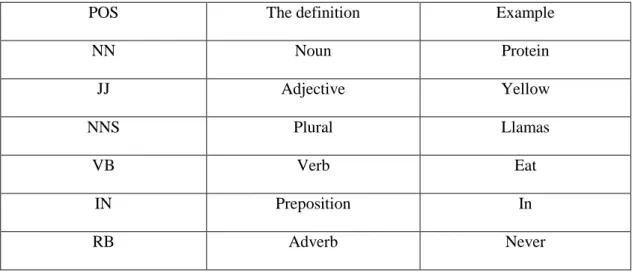
POS The definition Example

NN Noun Protein JJ Adjective Yellow NNS Plural Llamas VB Verb Eat IN Preposition In RB Adverb Never

13

3 Research Methods

The goal of the research process is to produce new knowledge or deepen understanding of a topic or issue. Hence, in order to create a new knowledge, or make the knowledge about a subject deeper, choosing the appropriate research method is necessary [37]. There are two main ways for research design: qualitative research and quantitative research [22]. One of these research design types are chosen by researches depending on the research problem which is going to be observed or the research question which is going to be answered [23]. Different steps of conducting this master thesis as a research are explained in this part.

In this master thesis we used design science methodology to present a design science research. Besides, we got much benefit of literature search for theoretical contribution in this subject and then the implementation method is used Java language in structured programming [34, 35].

Design science is a methodology in scientific researches which is mainly used in researches in the field of information systems (IS). This kind of researches focuses on development and performance of artifacts with a clear intention of improving the performance of artifacts [36].

Design process is consisting of some different phases which are defined by various DSR frameworks. These divisions of phases are done by specifying a set of milestones during the design process. These design science research method (DSR) frameworks usually launch repetitive approach including several phases of the design process. The example of this type can be referring to [24, 25].

These steps of DSR are illustrated as following [26]: 1. Awareness of the problem

2. Suggestion 3. Development 4. Evaluation 5. Conclusion

14

We have followed these steps for using the methodology in our master thesis. Below we have described how we have translated the five steps in the process of our work. Selection 3.1 to 3.5 explains how the structure has been fitted to the steps of design science methodology.

3.1

Awareness of the Problem: Literature Search

It is the first step in starting a research. By reading different literatures related to the subject we have chosen, the awareness of the problem was obtained for our research work. We started the research question for this matter. There is a research question which has been introduced in the beginning of a research and has been answered during that research [28]. Result of the literature review can formulate the problem and become a motivation to the research work. Using a relevant theory is helpful for applying some parts of the theory into the proposed theory. This needs reviewing the past literature.

Regarding our research questions and also implementing the proposed method, we reviewed relevant books and articles which were carefully selected by recently cited sources and authors.

Taking into consideration the role of literature review which is to develop theoretical framework and also conceptual models, the act of combining relevant elements from earlier studies is helpful [38]. Regarding this matter, we have motivated our work by paying attention to the researches done in this field.

In order to getting benefits of relevant researches, various literature which fit into our research area have been studied to get theoretical background knowledge such as GO, classification, Naïve Bayes, machine learning, as well as information regarding similar experiments. This information has been sought both from books on the topic and scientific reports and journals. Books have been found by searching the local and national library catalogues Higgins and Libras.

Finally by reviewing different of systems in the biomedical field, we developed the framework of our system which is illustrated in Figure 4-1 and later described in chapter 4.

15

3.2 Suggestion

Next step in providing a research is “suggestion” phase. This phase is necessarily used after recognizing the problem of research’s field and can be applicable after making a proposal as a output of the problem recognition [29]. Suggestions are the approaches including methods and methodologies which help the proposal to solve the mentioned problem.

By having suggestion’s definition in mind, the task of choosing an appropriate method reached us to the suggested following steps:

1) Developed the classification model

We proposed a classification model that identifies the roots of terms. There are two categories in our classification model: one category is tokens are marked into root, the other is tokens are not marked into root.

2) Chose the appropriate algorithm

We chose the Naïve Bayes algorithm and it is described in chapter 2.2.2. 3) Selected the features

With the help of our supervisor, we defined the four features as described in chapter 2.2.3. We have supported one new method for extracting the feature POS.

4) Selected the implementation and evaluation data

We chose the GO as our implementation and evaluation data

After these suggestions, we decided to use Java as our programming language and My eclipse 9.0 as our programming environment. In the suggestion phase we have described about development of system and the methodology we chose in next sections which are mainly mentioned in 3.3 and 4.2. According to this step, we recognized the need of requirements within system’s developing. Developing the suggestion’s step in the next phase which we have explained below [28, 39].

3.3 Development

This phase focuses on the development and implementation of the tentative design which was described previously in suggestion phase. Creative efforts are needed

16

while moving from tentative design into complete design requires. Developing and implementing approaches are different due to the differences in making artifacts, sometimes an algorithm is needed in order to build the development technique [30, 31].

In this master thesis, we developed a program for identifying the roots of terms according to our classification model. Our development environment was My eclipse 9.0 and programming language was Java.

In this master thesis, the main implementation is to implement the classification model for identifies the roots of terms. We need not develop a complete system like big software engineering project and only develop some specific programming for each parts implemented. With the help of our supervisor, we developed our implementation part according to the surprised machine learning process. This will be described in chapter 4 later.

3.4 Evaluation: Cross-validation

Evaluation is considered as an activity in software engineering to determine the quality of the proposed software. After developing the proposal, the output should be evaluated. The attention of evaluation phase is judging results according to performance and measurement of algorithm [40].

By searching various of papers about the evaluation method, we decided to use the cross-validation method. Cross-validation is a technique for assessing how the results of a statistical analysis will generalize an independent data set. It is mainly used in settings where the goal is prediction, and one wants to estimate how accurately a predictive model will perform in practice [32].

Cross-validation is widely used for evaluating training dataset and test dataset in machine learning. All the examples in the dataset contain training dataset and test dataset are eventually for both training and testing. The evaluation result has large persuasive.

17

3.5 Conclusion Phase

The conclusion phase is the last step in creating a design science research. The results are focused to the classification model for identifying the roots of terms. The main involvement of the conclusion is to achieve results, which are defined clearly in the purpose or objective of the proposal. We conclude after the evaluation phase from the domain experts and knowledge mentors, that the results are authentic and that they are truly mapped according to the purpose of this thesis.

The analysis of results, taken from evaluation leads us to have an overall understanding of our system. It can be conclude that how accurate is the system according to analyze the results.

18

4 Framework and practical methods

We presented the general framework that contains the whole process of supervised machine learning. Within this framework, we developed our system and implemented in GO.

4.1

Framework of supervised machine learning

method

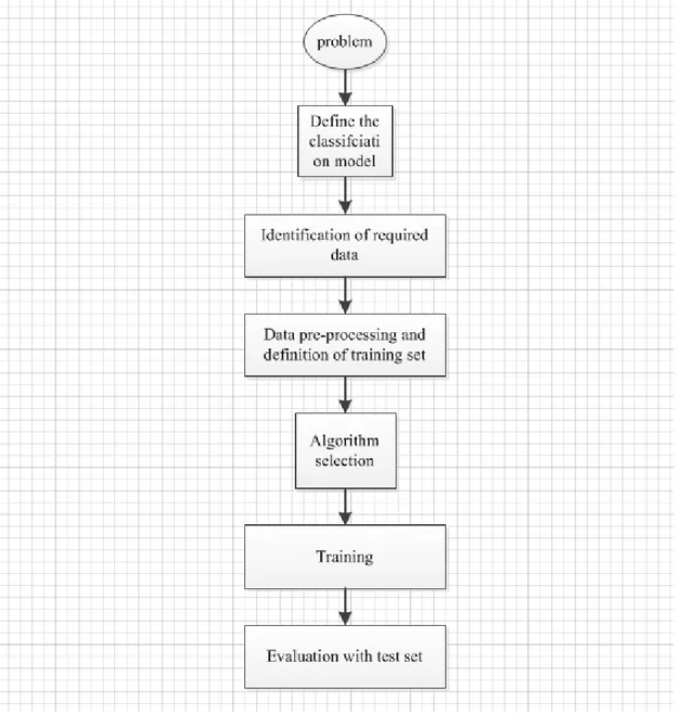
The overview of the supervised ML is illustrated in figure 4-1.

19

Regarding the literature, we found the framework of supervised ML method [3]. As the figure 4-1 shows, there are mainly four steps in the process of supervised ML in our thesis project. The first step is collecting the dataset, the second step includes the data preparation and data pre-processing, the third step includes algorithm selection and training, the last step is evaluation with test set.

 Problem

We first defined our problem that it is to identify the roots of terms by using the classification model.

 Define the classification model

20

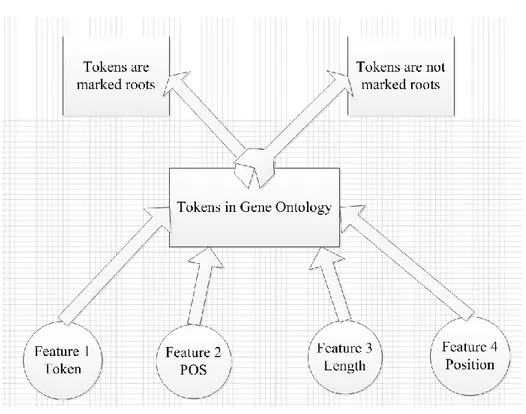
Regarding the literature and the help of our supervisor, we proposed the classification model as the figure 4-2 shown [43]. In figure 4-2, in our classification model, we defined four features: token, POS, length, position. The token means a word or other pares in lexical analysis. For example, for the term ‘transport protein’, the tokens are ‘transport’ and ‘protein’. The POS means POS of each token in its term. The Length means the length of a term. It is the number of tokens in a term. The position means a token’s position in its term. We defined two categories in our classification model. One category is that a token is recognized as root; the other category is that a token is recognized as not root. According to these four features, we used the Naïve Bayes algorithm to calculate the probability for each token as roots of terms. Compare these probabilities of tokens as roots and the biggest one token will be the root of term.

 Identification of required data

We chose the GO as our required data, because the GO was the biggest applications in the biomedical field. It covers different kinds of events in biomedical field.

Data pre-processing and definition of training set

After we decided to choose the GO as our required data, we did some pre-processing. Data pre-processing is an important step in the data mining process. The phrase “garbage in, garbage out” is particular applicable to data mining and machine learning projects. Data-gathering methods are often loosely controlled, resulting in out-of-range values, impossible data combinations, missing values, etc. Analysing data that has not been carefully screened for such problems can produce misleading results. Thus, the representation and quality of data is foremost before running an analysis. According to the classification model, we defined the training dataset.

 Algorithm selection

Regarding reading various of literatures, we chose the Naïve Bayes Algorithm for this thesis project.

21

After defined the training data set and selected the algorithm we would train our test dataset and do the evaluation with test data set. The training process is a classifier process.

In the selections that follow, we will describe step “identification of required data” to step “training and evaluation test set” in detail.

4.2

The development of system

4.2.1 Identification of required data and collecting the dataset

The first step is collecting the dataset. There are two normal cases for collecting the dataset. If an expert is available, then he or she could suggest which field is the most important. If not, then the simplest method is that of “brute-force”, which means measuring everything available in the hope that the informative and relevant features can be isolated [33].

In this master thesis, we combined these two cases for collecting dataset. With the help of our supervisor, she suggested the GO was the most informative ontology in biomedical field. In our literature search, we also found that the GO is the biggest application in text processing in biomedical field. Then we used the “brute-force” method defined the whole GO terms as our original dataset. Finally, we collected all 32464 terms in the GO. The GO version we used is GO-1.2. In this step, our input is GO-1.2 version txt file and output is all the terms of GO.

In this process, we did not consider the synonyms in GO. We only consider main terms.

4.2.2 Data preparation and data processing

4.2.2.1

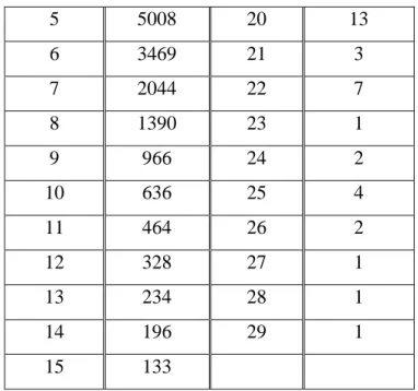
We carefully chose the dataset consider the length of terms. Length Numbers of terms Length Numbers of terms 1 512 16 110 2 4662 17 33 3 11673 18 25 4 6526 19 10

22 5 5008 20 13 6 3469 21 3 7 2044 22 7 8 1390 23 1 9 966 24 2 10 636 25 4 11 464 26 2 12 328 27 1 13 234 28 1 14 196 29 1 15 133

Table 4-3: The number of different lengths of GO terms

As the table 4-3 shown, there are many different lengths of GO terms. The length 3 terms has the most and there are few terms more than length 20. According to the table 4-3 shown, in order to cover the different lengths of terms in suitable dataset, we extracted the terms as array list order in the following proportions: the proportion of the terms length=1 and the numbers of the terms<=100 is 60% and the others are 10%. Because as the table 4-3 shown, the length=1 terms and the numbers of terms <=100 is short compared to other lengths terms. Our dataset should cover different lengths of terms. Finally we got the 4050 terms as our data set. In this step, the input is all the GO terms and the output is dataset with 4050 terms.

In dataset we chose, it covers different lengths of terms. The tokens of these terms have different POS, the same tokens have different positions in each term. It covers all the features we selected.

23

4.2.2.2 Extract the training set

For this step, our task is to get the training set. In machine learning theory, the training dataset should present representative features of dataset. According to the table 4-2, we extracted the training data set from the dataset we defined in 4.2.2.1 in the following proportion: the proportion is 100% that the length of terms is bigger than 18, the proportion is 10% that the length of terms is smaller than 18 . Thus our training set will cover all the different lengths of terms. Then we do the artificial classification for training set.

4.2.2.3 Extract the features of the dataset

For tokenization, we used the space symbol method for dividing the terms and did the further processing under handling some special symbols, i.e. “（”，“）” and “,” We did not handle the other special symbols.

For POS, we proposed an improved method based on the Brill Tagger. Brill Tagger is one POS method has high accuracy [21]. Brill rules are the general form: tag 1→tag 2 IF Condition, where the ‘condition’ tests the preceding and following word tokens, or their tags. For example, in Brill’s notation:

IN NN WDPREVTAG DT while

It would change the tag of word from IN to NN, if the preceding word’s tag is DT (determiner) and the word itself is “while”. Based on the existing rules in Brill Tagger, we developed some new rules based on the English grammars and some new rules based on the specification biomedical data. We also done some improvement for unknown-word algorithm based on Brill Tagger. We added more variables in program and used for while to improve the effecnicy of existing unknown-alforihm in Brill Tagger.

There are some new rules we added:

1. NN VB PREVTAG TO: it means when the TO is in pre-position of NN, then the NN should be changed to VB.

2. NN s fhassuf 1 NNS x means the unknown word was tagged NN, but the word end with “s”, it should change to NNS.

3. VB the fgoodright NN x means the unknown word was tagged VB, if this word is in the right of “The”, it should change to NN.

24

The tokens’ format in dictionary we used is: Token tag 1, tag 2, tag 3... tag n

Tag 1, tag 2…, tag n mean different tagging for each token possible. The tag 1 means the most possible tagging for this token. When the new token arrives, the program will look for the dictionary first. If the token is existed in the dictionary, this token will be marked as tag 1. If the token is not in the dictionary, then will use the unknown-word algorithm based on the rules we defined.

In unknown-word algorithm, first we used the information about word spelling for initialization. For example, the words ending in the letters “s” is most likely a plural noun and the words starting with an uppercase letter word is most likely noun and so on. After initialization and then do the POS tagging according to the rules we defined. For example, for term “Activation Of MARKKK During Sporulation Sensu Saccharomyces”, we got a protein POS tagging for each token according to dictionary, the protein of POS tagging is:

Activation: NN Of: IN MAPKKK: NN During: IN Sporulation: NN Sensu: NN Saccharomyces: NN.

Then we adjusted these results using the rules. For token saccharomyces, it is marked NN, but according to the rules NN s fhassuf 1 NNS x, it should be changed to NNS. Finally the term of POS tagging is:

Activation: NN Of: IN MAPKKK: NN During: IN Sporulation: NN Sensu: NN Saccharomyces: NNS.

We tested our improved POS method for data set and got 89.1% average accuracy. The accuracy means the proportion of the words were marked POS rightly in the whole words were marked POS.

For length, we used the “I” variable to control and count the numbers of tokens. The length is the numbers of tokens for each term.

For position, we used the array to present the different positions of each token in terms. We got all the features of the dataset. It shown table 4-4 in below:

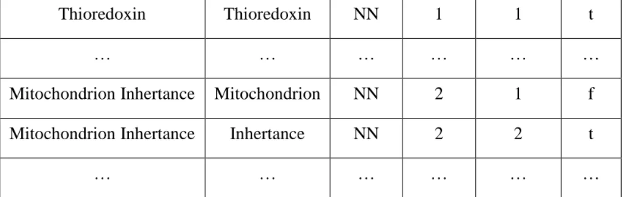
Term Token POS Length Position Root Reproducation Reproduction NN 1 1 t

25

Thioredoxin Thioredoxin NN 1 1 t

… … … …

Mitochondrion Inhertance Mitochondrion NN 2 1 f Mitochondrion Inhertance Inhertance NN 2 2 t

… … … …

Table 4-4: The features of the training set

For example, the term “Reproduction”, the POS NN means reproduction is noun, the length ‘1’ means the term has only one token and the position ‘1’ means the token ‘Reproducation’ is in the first position. In this step, our input is the dataset and the output is the dataset with features.

4.2.3 Algorithm selection and training

The choice of which specific learning algorithm we should use is a critical step. Once preliminary testing is judged to be satisfactory, the classifier (mapping from unlabeled instances to classes) is available for routine use. The classifier’s evaluation is most often based on prediction accuracy. In this master thesis, we chose the Naïve Bayes algorithm. Based on the literature, we found some advantages of Naïve Bayes algorithm. It has the faster speed for learning with respect to numbers of attributes and the numbers of instances, the faster speed of classification, tolerance to missing values are better [18].

Based on the classification model, our target value is given by the following formula in the equation 4-5 based on the equation 2-4 in chapter 2:

) " " | ( ) " " | ( ) " " ( max arg 4 2 i i j 1 } . { t root features P t root token features P t root P T tokens terms token root j     



Equation 4-5: The target formula is based on the Naïve Bayes algorithm [19] There is a description of the formula shown in equation 4-5:

(1) P(root="t"), this is the proportion that the tokens features are “t” in the whole training set token.

26 then 150 50 10 * 5 10 * 4 10 * 3 10 * 2 10 * 1 50 ) " " (        t root P

(2) P(token=A| root="t"), this is the proportion that the tokens features are “t” and token feature=A in the whole tokens are treated as roots in the training set

(3) P(POS=B| root="t"), this is the proportion that the tokens features are “t” and POS feature=B in the whole tokens are treated as roots in the training set.

(4) P(length=C| root="t"), this is the proportion that the tokens features are “t” and length feature=C in the whole tokens are treated as roots in the training set.

(5) P(position=D| root="t"), this is the proportion that the tokens features are “t” and position feature=D in the whole tokens are treated as roots in the training set.

For example, we want to identify the root in the term “endopolyphosphatase activity”, according to our formula:

For endopolyphosphatase, the probability of root is:

) " " | 1 ( ) " " | 2 ( ) " " | " " ( ) " " | " ( ) " " ( t root positon P t root length P t root NN POS P t root osphatase endopolyph token P t root P         

It is based on the equation 4-5.

For activity, the probability of root is:

) " " | 2 ( ) " " | 2 ( ) " " | " " ( ) " " | " " ( ) " " ( t root positon P t root length P t root NN POS P t root activity token P t root P         

There is an example how to calculate the probability for each part. For example,

P(token="activity" | root="t"), it is the proportion that the numbers of activity token

are treated as roots in the training data set. For example, the training data we used contains 453 terms. There are 453 roots in the training data set and in case 70 of roots is “activity”, then we get

453 70 ) |

(tokenactivity roott  P

27

Finally, we got the two probabilities for token ‘activity’ and ‘endopolyhosphatase’, compare these two probabilities, the token activity’s probability is bigger than endopolyphosphatase’s probability and the root will be ‘activity’. There is a special case for P(token="activity" | root="t"), if the token activity is never occurs in the training dataset, the probability will be zero. Then we used the Laplace smoothing for correction this case. If a given class and feature value never occurs together in the training data, we will all one smoothing parameter ‘a’. The ‘a’ is equals one. That means each given class and feature at least occurs one times in the training data. It will be avoid the case of probabiluty zero. In our classification model, there are 453 training terms. There are 453 roots in the training dataset and in case 0 of roots is ‘transport’, we will assume the ‘transport’ occurs one times, and then calculate the probabilities.

4.2.4 Evaluation with test set

In this step, our task is to evaluate the test data set according to cross-validation method. Cross-validation is a technique for assessing how the results of a statistical analysis will generalize an independent data set. It is mainly used in settings where the goal is prediction, and one wants to estimate how accurately a predictive model will perform in practice [32].

In our experiment, we used the improve hold-out method. We divide our data set into two parts. One part training data set, the other one is test dataset. Then divide the test dataset into 9 parts and test each part. Then get the 9 set results and calculate the average accuracy. The test dataset contains some synonyms.

In this step, the input is the 9 test set files, the output is 9 test set files with possibility and 9 test files without probability.

4.2.5 Implementation

For this paper, we used the Myeclipse as our development tool and implemented in Java program. There are 4 mainly parts in our implementation. First part is for selecting dataset, second part is for selecting training dataset, third part is for selecting dataset with features, fourth part is for testing data set.

28

5 Results

This section presents the practical results of our work which we have done during this master thesis. It also states how the objective of this thesis work is reached according to the development process. Once the objective is achieved, the result is ready. The results show how to identify the roots of terms step by step [34].

5.1 Practical Results

In this selection, we explain the results according to the development of process. Below you can review the results:

 Figure 5-1 and Figure 5-2 showed the dataset collected

 Figure 5-3 and Figure 5-4 showed the dataset with figures

 Figure 5-5 showed the training dataset with classified

 Figure 5-6 showed test dataset 1 with probability

 Figure 5-7 showed test dataset 1 without probability

29

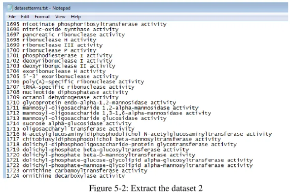
Figure 5-2: Extract the dataset 2

Figure 5-1 and figure 5-2 shows a small subset of data set which contains 4165 GO terms we choose. In machine learning theory, the quality of dataset has the directly effect on the final results. Thus, our dataset should cover all the lengths of terms according to features we choose. As the figure 5-2 shown, we also can know the same token probably have the different positions in different terms. For example, as figure 5-2 shown, for term 1696 ‘nitric-oxide synthase activity’, the token ‘activity’ position is 3 , as figure 5-1 shown, for term 313 ‘lactase activity’, the token ‘activity’ position is 2.

The figure 5-3 shows a small subset of the data set with features. This result is shown we have succeeded extracting all the features we used: token, POS, length, position, and root. For example, as the figure 5-3 shown, for number 1 term ‘reproduction:NN:1:1:T’, NN means reproduction is Noun, the first ‘1’ means the term has one token, the second ‘1’ means the token reproduction’s position is 1. T means ‘reproduction’ was marked root.

30

Figure 5-3: Extract the dataset 1 with features

Figure 5-4: Extract the dataset 2 with features

The figure 5-4 is shown a small subset of training dataset without annotations. As the figure 5-4 shown, the training dataset have not annotated yet. All the terms (length is bigger than 1)’s roots were marked into “f”.

31

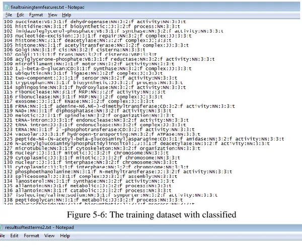
The figure 5-6 is shown our training data set with the annotations. According to the supervised machine learning method, the class should be pre-defined. After extracting the training data set shown in figure 5-4, we classified the training data set and got the training data set with annotations shown in figure 5-6.

As the figure 5-6 shown, for number 101 term ‘histidine:NN:3:1:f biosynthetic:JJ:3:2:f process:NN:3:3:t’, token ‘histidine’ NN means POS was marked NN(noun), ‘3’ means this term has three tokens, ‘1’ means the token ‘histidine’ is in the first position, ‘f’ means the token ‘histidine’ was not marked root.

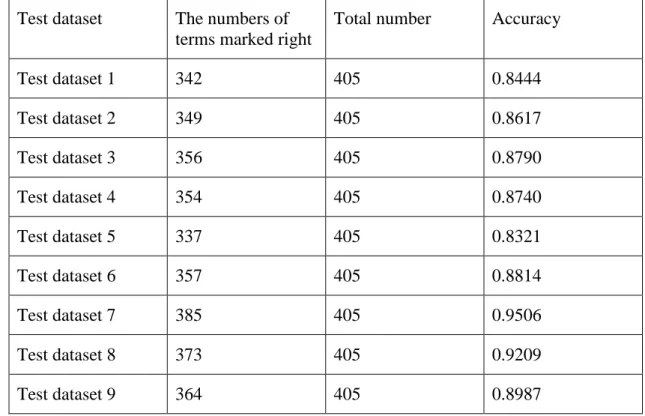
There are 453 terms in our training data set. Then we divide the rest data set into 9 test data set and each test data set has 405 terms. Finally we get 18 test data sets results, 9 test data sets with possibility and the other 9 test data sets without possibility. We also can see the accuracy for each test data set from the result. The accuracy is defined as the proportion that the right numbers of terms marked as roots in test data set. The accuracy is calculated in following equation 5-5:

The right numbers of terms marked as roots Accuracy =

numbers of terms in each test dataset

Equation 5-5: The accuracy calculation formula

Figure 5-7 showed test dataset 1 with probability. For example, in figure 5-7, for term ‘radial: 4.749670099285197E-10 spokehead: 3.9752693418534165E-9 ROOT: spokehead’, spokehead: 3.9752693418534165E-9 means the probability that token ‘spkoehead’ was recognized the roots for this term was 3.9752693418534165E-9. It is bigger than 4.749670099285197E-10. So this token ‘transport’ is the root for this term. Figure 5-8 showed the test dataset 1 without probability. For example, in figure 5-8, for number 114 term ‘guanine nucleotide transport’, the root is transport.

There are some terms were marked wrong roots. For example, in figure 5-8, for number 115 term ‘skeletal system development’, we marked the token ‘system’ into root, but the real root should be ‘development’. Our results not only show the roots of terms effectively, but also can show the Exact Root of terms was marked wrong. The table 5-9 shows the accuracy of 9 sets of test data set. We got 9 test data files without possibility and 9 test data files with possibility and got the 88.25% average accuracy.

32

Figure 5-6: The training dataset with classified

33

Figure 5-8: The final test dataset 1 without possibility

Test dataset The numbers of terms marked right

Total number Accuracy

Test dataset 1 342 405 0.8444 Test dataset 2 349 405 0.8617 Test dataset 3 356 405 0.8790 Test dataset 4 354 405 0.8740 Test dataset 5 337 405 0.8321 Test dataset 6 357 405 0.8814 Test dataset 7 385 405 0.9506 Test dataset 8 373 405 0.9209 Test dataset 9 364 405 0.8987

34

6 Analysis and discussion

6.1

Analysis the results based on the method for

extracting the features

In machine learning methods, the method for extracting the features has the effected on the final results.

For feature tokenization, we used space method in java for tokenization. This method cannot avoid some deviation. It has limitation that avoiding all the special symbols of terms.

For feature POS, we used improved Brill Tagger method. However, this method is not perfect, we cannot avoid some mistakes in using this method. We calculated the numbers of tokens which were marked wrong POS. By accounting, for the training data set we chose, there are 2434 tokens, the numbers of tokens were marked wrong POS were 249, the accuracy is about 0.8971. This accuracy is defined as the proportion that the tokens marked POS rightly in the whole tokens.

35

As the figure 6-1 shown, the italic tokens mean which were marked wrong POS. For example, for term 53 ‘SAGA complex’, the token ‘complex’ was marked JJ and its real POS should be NN.

The quality of method used for tokenization will decide how many tokens we can get in the dataset. For the feature length, it is based on how many tokens we can get. Thus, the method’s quality of tokenization will also have effect on the feature length. For position, we used the array to define the tokens’ position. The array’s length is the numbers of tokens in each term. It is based on how many tokens we got according to the tokenization. Thus, the quality of tokenization also has the effect on the feature position.

Therefore, the method for extracting the features has the effect on the quality and accuracy of classification.

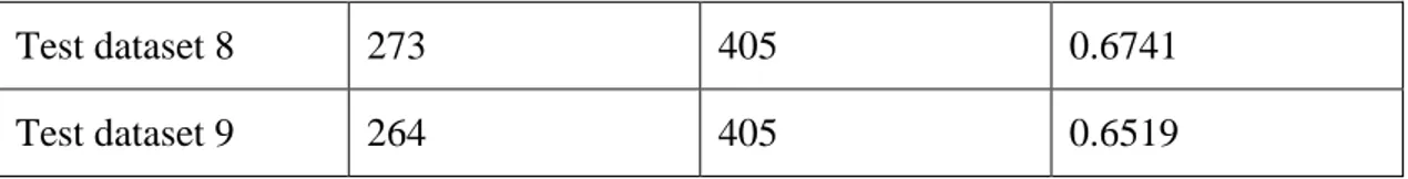
6.2 Analysis the results based on the size of training

data set

As the table 6-2 shown, the training data set has 453 terms. It covers different features mentioned in classification model. If we changed the training data set from 453 terms into 200 terms and the new training data set not covered all the different features, we found the new test data set results have low accuracy. This is indicated that the quality and chose of training data set is important and has a directly effect on the quality of classification model.

Test dataset The numbers of terms marked right

Total number Accuracy

Test dataset 1 242 405 0.5975 Test dataset 2 249 405 0.6148 Test dataset 3 256 405 0.6321 Test dataset 4 254 405 0.6272 Test dataset 5 237 405 0.5852 Test dataset 6 257 405 0.6346 Test dataset 7 285 405 0.7037

36

Test dataset 8 273 405 0.6741 Test dataset 9 264 405 0.6519

Table 6-2: The test data set result with training data with 200 terms

6.3 Analyse the results based on the final test data

result

As the table 5-9 shown, the test data set has got an effective average accuracy 88.25%. But there are still some terms were marked into wrong roots. For test data set 1, there are 63 terms were marked into wrong. By accounting, there are 14 terms were marked into wrong may because the tokens were not in the training dataset. For example, for term ‘protein: 6.964703613691954E-6 deneddylation: 3.96570213123213E-5 ROOT: protein’, the exact root is deneddylation. It may because the token deneddylation is not in the training data set and the training dataset has the limitation of size that it cannot cover all types of terms.

There are 25 terms were marked into wrong may because the tokens were marked into wrong POS. For example, for term ‘transition: 2.894340388125493E-5 pore: 1.894340388125493E-5 complex: 1.79734039127896E-5 ROOT: transition’, the exact root is complex. We marked the JJ for token ‘complex’, the real POS is NN. Therefore we got the wrong root.

There are 24 terms were marked into wrong because of model error. Our classification model for identify the roots is not perfect, it cannot avoid the error. For example, for term ‘urogenital: 0.0 system: 2.0657645123091753E-5 development: 3.45789213212354E-5 ROOT: system’, we checked each token’s POS is right and the exact root is ‘development’. However the token ‘development’ probability is bigger than token ‘system’, but we marked ‘system’ into root. It may because of system error.

Test data set The numbers of terms

marked wrong The numbers of terms marked wrong (Model error maybe) The numbers of terms marked wrong (POS error maybe) The numbers of terms marked wrong (Training set error maybe)

37

Test data set 2 56 11 23 22

Test data set 3 49 9 21 19

Test data set 4 51 10 21 20

Test data set 5 68 17 28 23

Test data set 6 48 10 20 18

Test data set 7 20 5 8 7

Test data set 8 32 8 13 11

Test data set 9 41 11 16 14

Table 6-3: The terms marked wrong in three ways

As the table 6-3 shown, there are three causes that the roots were marked into wrong. Most terms were marked into wrong probably because the wrong POS and training dataset error.

38

7 Conclusion and Future work

The first research question “What is the method for identification of the roots of terms” was finely answered in chapter 2, 4 as well as second question “What general framework is needed regarding support of the method”.

In this master thesis, we determined the method for classification. According to classification model, we divide two categories, one is that token was recognized as roots and the other one is that token was not recognized as roots. Based on the four features, we calculate and compare the probabilities for each token. Finally we identify the roots of each term. This is our theoretical process for how to identify the roots of terms.

This master thesis can be seen as a step towards to analysis of the compositional structure of terms in biomedical field. The proposed general classification model which aims to identify the roots of terms in biomedical field was implemented in GO. The proposed framework of supervised machine learning can be tailored to any biomedical ontology.

Our classification model got the satisfactory results. In particular, we develop an effective POS method based on Brill tagging method. We have succeed in generating a general method for identify the roots of terms in biomedical and implemented in GO.

Our method is depending on the quality of classification model and algorithm for calculating the probability. Following our result, future work could possibly improve our classification model and try to use other algorithm. In our project, we only identify the roots of terms. We will analyse the compositional structure of terms not just roots in the further work. For POS, we will improve our rule-based POS method in future research.

In short, we have succeed in generating a classification model that judging which token is root in GO used the Naïve Bayes algorithm. The model got the effective result. In future work, we will try to use the other field’s data for implemented and use the other algorithms for calculating the probabilities. Then compare the difference to the Naïve Bayes algorithm. Finally we will do the term parsing according to this master thesis.