Operating with Options : A Study of Volatility

J

I

B

S

JÖNKÖPING UNIVERSITY

O p e r a t i n g w i t h O p t i o n s

A Study of Volatility

Master thesis in economics Author: Martin Berntsson Tutors: PhD Johan Klaesson

Master Thesis in Economics

Title: Operating with Options – A Study of Volatility

Author: Martin Berntsson

Tutor: PhD Johan Klaesson and PhD. Candidate Johanna Palmberg

Date: September 2006

Subject terms: Black-Scholes, Volatility, Options, Finance, Strategies

Abstract

In this thesis, I have had the intention to try to explain the importance of having a concep-tion of volatility when one is trading with Opconcep-tions. The purpose has been to investigate if one can learn anything from the history of the volatility and to study if the historical volatil-ity is a better indicator of the future volatilvolatil-ity than the implied volatilvolatil-ity. Additionally, to see if one can make a profit from Options with a different conception of the volatility.

In the thesis, I have used Black, Scholes and Merton’s epoch-making theory on how to price Options, the Black-Scholes formula. From that formula, I have derived the volatility in the OMX index’s Option prices, the implied volatility. I have also used the formula to calculate the true and historical volatility. In order to take advantages from a different con-ception of the future volatility than the markets I have presented a number of different Option strategies.

The conclusions I have been able to draw from OMX index Options in year 2001 is that the implied volatility seems to be better to predict the true volatility than the historical vola-tility. Neither one of them is perfect indicators of the true volatility but the total sums of squares of the implied volatility deviates less from the true volatility than the historical volatility on average.

To conclude the history of the volatility one can establish the fact that the volatility that re-flects in Option prices does not very often correspond with the true volatility. No one have the power or the insight to prognosticate the future volatility perfectly incessantly. Yet, it is the differences in people’s conceptions of the volatility that create the trade with Option and makes it to such an interesting and useful tool.

Magisteruppsats inom Finansiering

Titel: Operating with Options – A Study of Volatility

Författare: Martin Berntsson

Handledare: PhD Johan Klaesson and PhD. Candidate Johanna Palmberg

Datum: September 2006

Ämnesord: Black-Scholes, Volatilitet, Optioner, Finansiering, Strategier

Sammanfatting

I denna uppsats har jag haft intentionen att försöka förklara vikten av att ha en uppfattning av volatilitet när man handlar med Optioner. Syftet har varit att analysera ifall man kan lära sig från volatilitetens historia, och ifall historisk volatilitet är bättre på att indikera framtida volatilitet än marknadens volatilitet, även kallad den implicita volatiliteten. Syftet har även varit att undersöka ifall det går att göra vinst på Optioner om man har en annan uppfatt-ning om den framtida volailiteten.

I uppsatsen har jag använt mig av Black, Scholes and Mertons epokavgörande teori om hur man prissätter Optioner, den så kallade Black-Scholes ekvationen. Från den ekvationen har jag erhålligt volailiteten i OMX index Optioner, den implicita volatiliteten. Black-Scholes ekvationen har likaså använts för att härleda denna faktiska och historiska volaliteten. För att kunna utnyttja en annan uppfattning om den framtida volaliteten än marknadens så har jag presenterat ett antal olika Options strategier.

De slutsatser som jag har kunnat dra från år 2001 OMX index Optioner är att den implicita volaliteten verkar vara bättre på att förutspå den faktiska volaliteten än den historiska vola-tiliteten. Ingen av dem är en perfekt indikator på den faktiska volatiliteten men i genomsnitt så skiljer sig den implicita mindre från den faktiska än den historiska.

För att sammanfatta volalitetens historia så kan man påstå att volatiliteten som reflekteras i Optionspriset sällan stämmer överens med den faktiska volatiliteten. Ingen sitter på Op-tionsmarknaden med en kristallkula och kan förutspå volatiliteten perfekt hela tiden. Sam-tidigt är det just skillnader i volatilitetstro mellan de olika aktörerna i en Optionsaffär som skapar handel och som gör Optioner till ett så användbart och intressant instrument.

Table of Contents

1

Introduction ... 1

2

Options... 4

2.1 Basic Terminology about Options ...4

2.2 Risk with Options ...6

2.3 Strategies with Options ...7

2.3.1 Bull Spreads ...8 2.3.2 Bear Spread...9 2.3.3 Butterfly Spreads ...9 2.3.4 Bottom Straddle ...10 2.3.5 Top Straddle ...11 2.3.6 Bottom Strangle...11 2.3.7 Top Strangle ...12

3

Method ... 14

3.1 The Black-Scholes Formula ...14

3.2 Assumptions about Black-Scholes Formula...15

3.3 Volatility...15

3.4 Selection Process ...16

3.5 Calculate the Volatility ...16

3.6 The Risk-free Interest Rate...17

3.7 Deviation...17

4

Result and Analysis ... 18

5

Conclusions and Further Research ... 25

1

Introduction

The world’s financial market does not only consist of trade with shares as many people might assume, it has for the last 20 years had an increasing trade with derivatives. Deriva-tives can be defined as a financial instrument whose value depends on the values of other assets i.e. price of a share, rate of a bond or the rate of exchange. The most common used derivatives are Options, Futures, Forward contracts and Swaps.

Options are believed to have existed as far back as thousands years ago but more generally, trade with Options is thought to be commonly used first around the seventeen century in Holland. By that time, Option contracts were made with tulip bulb as underlying assets. During the nineteen century and up until today, farmers have used Options to insure that their harvest would be sold for a certain price. It was first in the 1960’s when Option with financial securities as underlying assets started to be traded (OMX Stockholm., 2002). In 1973 when Chicago Board Options Exchange started to trade with Options and introduc-ing standardised contract, it became widely known and used around the world. Today, trade with standardised Forward contracts and Options can be found on many of the world’s financial markets. Nevertheless, all trade with derivatives is not standardised con-tracts, a large part of the trade takes place in the OTC (Over The Counter) market. With an OTC-contract a derivative instrument will be establish as a separate contract between two operators (Hagerud G., 2002).

The difference with Options and other derivatives is that the holder of an Option has the right to exercise the contract whereas the holder of for example Forwards or Futures is ob-ligated to exercise the contract. For this right the holder of an Option has to pay a premium, a form of compensation to the issuer while forwards and futures are costless to enter (Hull J. C., 2006).

Questions that usually comes to mind considering Options are, how Options is priced, un-der what circumstance should one consiun-der to buy call or put options or sell call or put op-tions?

Since 1973 when Black, Scholes and Merton presented their epoch-making theory on how to price Options, brokers, investor and securities trader have used it. To be able to calculate the value, hence the price of an Option by using Black-Scholes theory, one would have to observe or estimate five different variables. These variables are; the price of the underlying asset, the exercise price, the time to maturity, the risk-free interest rate and the volatility of the underlying asset. The share price, the exercise price and the time of maturity could all be observed. For the risk-free interest rate, one usually uses a treasury bond with the same time of maturity as the Option. When it comes to the volatility of the underlying asset, some estimation must be made and it is here the “problem” starts. Black-Scholes assume that the volatility is known and constant. This is a stringent condition to be made on fi-nancial data, especially since one could quite easily prove the opposite (Black and Scholes, 1973).

There are four types of volatility: historical, implied, prognosticated and true (future). His-torical volatility is always a good starting point to prognosticate the future volatility and also to obtain an apprehension if the implied volatility, which the market use to set the Option price, is within a reasonable spread. However, the historical and the implied volatility is of-ten not the same as the future, true volatility.

It is very difficult to make perfect prognostication of the future volatility. Professional op-erators apply very sophisticated statistical models i.e. GARCH-1 and EWMA-models2, some looks at histograms of historical and implied volatility or use “FingerSpitzgefuhl3” or “Guts-feeling3

” to estimate the future volatility. As hard, it is to prognosticate the volatility as hard it is to say which method that is the best one. However, in order to be successful it is important to consider the volatility. To have a conception of the volatility is actually the most crucial thing when trading with Options. Trading with options are the same as trading with risk i.e. to buy or sell risk and it is the differences of trader’s volatility conception that creates the market for Options and that is what makes Options to such a useful and inter-esting financial instrument (OMX Stockholm., 2002).

1.1

Previous Studies

The majority of the previous studies about Options like for example Black and Scholes ar-ticle “The Valuation of Option Contracts and a Test of Markets Efficiency” (1972) and Galai’s article “Tests of Market Efficiency of the Chicago Board Options Exchange” (1977) are written from the perspective of market efficiency. According to efficient market hypothesis, as prices respond only to information available in the market, and, because all market participants are privy to the same information, no one will have the ability to out-profit anyone else. Prices in an efficient market do not become predictable but random and investments strategies are therefore useless. Counter arguments to efficient market hy-pothesis state that consistent pattern are present and investments strategies are therefore a useful tool to beat the market. As Black, Scholes and Galai came to the same conclusion of a non-efficient market, that assumption will be regarded throughout this thesis.

There have also been studies about implied price of Options verses Black & Scholes price of Options. If the implied price has been over- or undervalue regarding to the price derived from Black and Scholes formula. Which of course originate in the differences of estimating the volatility of the underlying asset. Black and Scholes (1972) found that using past data to estimate the volatility caused the formula to overvalue the Options on high volatility assets and undervalue Options on low volatility assets. This thesis will therefore put emphasis on the volatility but from another perspective.

1.2

Purpose

Considering the importance of estimating the volatility when trading with Options, the purpose of this thesis is to investigate if one can learn anything from the history of the volatility. Is the historical volatility when using Black-Scholes assumption of constant vola-tility better to predict the true (future) volavola-tility than the implied volavola-tility? Can anyone make profits with a different conception of the future volatility?

1 _{The GARCH-model is dealing with a non-constant volatility, will not be explained in this thesis.}

2 _{EWMA or exponentially weighted moving average is models that recognize that volatilities are not constant.}

Engle R (1982).

1.3

Outline

This paper has been structured into five parts. After the first introduction chapter, the risk of option and a few suitable strategies will be explained in chapter two. Black-Scholes for-mula with its assumption will be presented in chapter three along with the thesis method. The Method of this thesis analysis is described in chapter four. The result of the analysis in Chapter four will be summed up into conclusions in Chapter five.

2

Options

This chapter will introduce the basic concept about Options, the risk with Options and dif-ferent strategies to use when operators has a difdif-ferent conception of the future volatility.

2.1

Basic Terminology about Options

There are two basic types of Options, call and put Options. A call Option gives the holder the right to buy the underlying asset (i.e. a share) for a predetermined price. A put Option gives the holder the right to sell the underlying asset for a predetermined price.

The seller of a call, also called the writer of the call, is obligated to deliver the underlying as-set at the predetermined price, called striking price or exercise price, on or before the spe-cific date if the holder of the call chooses to exercise it. A call Option is said to be a cov-ered call when the writer owns the asset that might have to be delivcov-ered upon exercise. A call Option is naked when the writer does not hold the underlying asset. Option based on indexes is always naked because the writer is only obligated to pay the differential amount of money if it is exercised and not the index “assets”, this is done of simplicity reason. A put Option is covered if the writer has a short position (agrees to sell) of the underlying as-set. The reason to have cover Options is to get a better return than one thinks the underly-ing asset would yield (Chance D. M., 1995).

An owner or holder of an Option (who is said to take a long position) acquires the Option by paying a premium (also called the Option price) to the writer (who is said to take a short position). If the holder of a call Option decides to exercise the Option, the exercise price is paid to the call writer in exchange for the underlying asset. If the holder of a put Option decides to exercise the Option, the underlying asset is delivered to the put writer in ex-change for the exercise price. Hence, there are four types of using Options, you are either a holder or a writer. The holder can either buy a call or put Option and a writer can either sell a call or a put Option (Chance D. M., 1995).

An individual that has good prospects of the market should take a short position of call Options and/or take a long position of put Options. If the individual has bad prospects of the market he should take a short position of put Options and/or a long position of call Options.

A person who takes a long position of a call/put Option is buying the right to buy/sell the underlying asset to the exercise price. A call Option that has shares as underlying assets will be exercised if the share price at the exercise day is above the exercise price. Because then the value of the Option is positive and allows one to buy the shares to a cheaper price than the market price. A put Option in this case would be worthless and the loss would be the same as the premium (Option price) (Chance D. M., 1995).

If the opposite occurs and the share price at the exercise day was below the exercise price, put Option would be exercised since it would give a positive value. One would than be able to sell the shares to a higher price than the market price. A call Option in this case would be worthless and the loss would be the same as the premium (Chance D. M., 1995).

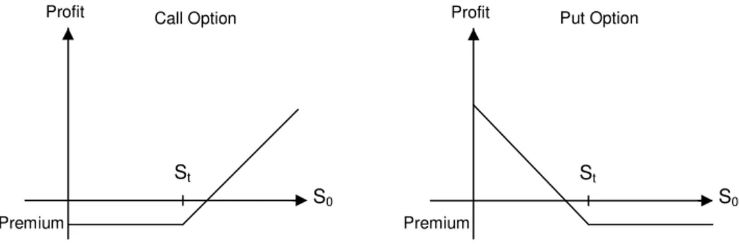
Figure 1 illustrates the profits of call and put Options, upon exercise, for long positions. The exercise of a call Option by its holders involves the purchase of the underlying asset at the St (exercise price).

Figure 1. Profits at exercise for call and put options (long position). Source: (Hull J. C., 2006)

The exercise of a call Option would therefore only occur if the market price of the asset (S0) is at least as great as St. Hence, S0≥ St should hold for a call Option to be exercised and

the profit would than equal S0-(St+Premium). The premium is, as mention earlier, the price

the holder of the Option has to pay (the Option price). The profit possibilities are unlim-ited and the risk is equal to the cost of the premium (Bailey R. E., 2005).

The exercise price of a put Option involves the sale of the underlying asset, by the writer to the holder of the Option at exercise price St. The exercise of a put Option would therefore

only occur if St is at least as great as S0. Hence, St≥ S0 should hold for a put Option to be

exercised and the profit would than equal St-(S0+Premium). The profit possibilities are

equal to the exercise price and the risk is equal to the cost of the premium (Bailey R. E., 2005).

One should bear in mind that this is in absence of any market frictions such as transactions costs incurred from buying or selling Options. If S0-(St+Premium), for a call option, is

smaller than the transaction cost of selling the asset then the Option may be unexercised. On the contrary if the investor wants to hold on to the asset following the exercise day he might be prepared to exercise the Option even if S0-(St+Premium)<0, because it could be

more expensive to buy the asset on the open market (Hull J. C., 2006).

Figure 2 shows the profit from the writer’s perspective, a so called short position of call and put Options. Short position is the opposite to long position, the exercise of a call Op-tion requires the writer to sell the underlying asset to the OpOp-tion holder at St.

Figure 2. Profits at exercise for call and put options (short position). Source: (Hull J. C., 2006)

The Option would only be exercised if S0≥ St and as mention before the writer will only

gain profit when the Option is not exercised. Hence, a writer’s profit equals the premium.

Profit

St Premium

Call Option Profit

Premium St Put Option Profit St Premium Profit St Premium Put Option S0 S0 Call Option S0 S0

The profit possibilities are equal to the premium and the potential risk is in principle unlim-ited (Bailey R. E., 2005).

Exercising a put Option requires the writer to purchase the underlying asset from the Op-tion holder at price St but the Option will only be exercised if St≥ S0. The writers profit

de-pends if the Option is exercised or not, if it is not exercised the writer will gain the pre-mium. The risk for the writer of a put option is equal to (St-S0)-Premium (Bailey R. E.,

2005).

Options are referred to “in-the-money”, “at-the-money” and “out-of-the-money”. An Op-tion that is “in-the-money” would give the holder a positive return if it were exercised im-mediately. An “at-the-money” Option would give the holder zero return and an “out-of-the-money” Option will give the holder a negative return if it were exercised immediately. Hence, a put Option would be “in-the-money” if the underlying price of the asset were above the strike price, if the price were below the strike price it would be “out-of-the-money” and if the price were the same as the strike price the put Option would be an “at-the-money” Option. An Option that remains “out-of-“at-the-money” until the exercise date will not be exercised. It is also therefore an “out-of-the-money” Option is the cheapest one to buy (OMX Stockholm., 2002).

2.2

Risk with Options

It is a difficult task to define risk. Variance of outcomes or volatility has many times been a common substitute for risk in finance. Volatility implies incomplete information and is of-ten used alone as an objective measure of inability to predict outcomes. Inability of predict-ing outcomes is often understood like somethpredict-ing unpleasant and somethpredict-ing that many people tries to avoid. Nerveless’, risk is something that we constantly confronts with, espe-cially when dealing with Options, so one are almost forced to try to define it or at least deal with it (Baird and Thomas, 1985).

Baird and Thomas (1985) thought of risk as a point of departure from two components, uncertainty and exposure of the same uncertainty. They also thought that people had dif-ferent preferences towards risk and that they therefore make difdif-ferent decision when they face the same choice. All information can be used to reduce the uncertainty and by that re-duce the risk in different situations. Some information has less significance in one situation while it has a major significance in another. A conclusion regarding information is how relevant it is to the object that lie behind the decision. While some people can be indiffer-ent towards an outcome of a special evindiffer-ent, others can be deeply influenced. The ones who are not influence by the outcome of the event are not exposed of any risk, that person does only stand in front of uncertainty. Hence, risk is something subjective and very hard to es-timate. Henceforth, the risk will only be considered as incidents that causes measurable economical loss in this thesis, such as movements of the underlying asset (volatility). Risk can be divided into two different categories:

• Nonsystematic risk, also called residual or diversified risk, is the risk that is unique for one company. Examples of this is unfavourable legislation, strikes but above all a company’s fall grounded on i.e. changed of markets preference or new competi-tors (Ross et al., 2005).

• Systematic risk is the same as market risk or risk that is not possible to undiversi-fied. It arises from a correlation between returns from the investment and returns

from the stock market as a whole. Economic collapse, war, interest level and po-litical instability can all be seen as a systematic risk (Ross et al., 2005).

Options are often financial instrument associated with much risk. Many people see it there-fore as an instrument exclusively used by large investors. Options are in them self very volatile instrument and can therefore be full of risk but most of the risk is known. If one buys a put or a call Option the maximum loss if the Option is not exercised will be equal to the premium. If one instead trades as a writer of a call Option and does not hold the un-derlying asset the loss will be uncertain. The holder has obligations and will be claimed to leave security on a reserve account (security margin). What amount the holder has to leave depends on how much the underlying asset changes from day to day until the maturity day. This will cause a liquidity risk, even if one in the end have the right prediction they may be forced to leave the position as a holder due to short term liquidity problems (McMillan L. G., 1992).

The derivative market is a market for redistribution of risks. The one who wants to reduce the risk of owning shares can do that and the one who would like to speculate in the mar-kets with a higher leverage than with shares can also do that. In that sense, the derivative market contributes to a more efficient financial market (Hull J. C., 2006).

There are often said to be three types of operators on the derivative market: speculators, hedgers and arbitrager. A speculator is often a private person or a company who takes high risks to get a high rate of return. The hedger, can be an institution or a fund, is the one who sells the risk to reduce the volatility in the result of the asset. The arbitrary, who often is the market maker, tries to be risk neutral and gain profit from the difference between the bid and ask price. All three types of operators are needed for a successful market. The hedger needs the speculator to be able to reduce the risk and vice versa. In the meanwhile, both groups need the market maker to match the need of the risk relocation (Hull J. C., 2006). Notice that the derivative market is a market where one can both measure and trade the ac-tual risk. Even if the share price is very dependent on the operator’s expectations of the risk, the risk premium will never be shown on the stock market. On the Option market, one can use Black-Scholes formula4

to calculate the implied volatility, which is the meas-urement of how large movements the Option market believe a given underlying asset will have until the maturity day. Hence, if risk is defined as volatility, it is easier to calculate the risk on the Option market than in the stock market and trading with Options should there-fore not be seen as riskier than trading with shares.

2.3

Strategies with Options

There are endless of opportunities to create various Option strategies. A trader can com-bine different Options depending on their prospect of the market and for what purpose he/she wants to trade. There are strategies for those who want to add the possibilities of a higher return on their portfolios but also for those who want to reduce the risk that arise at the stock market. Combinations of different Options and with various maturities can be used for investor that wants to follow their prospects and customise the risk exposure after their own preference. Investor’s often takes advantage of the leverage of Option to reduce

the risk in i.e. an share portfolio with help of a relatively small initial investment (McMillan L. G., 1992).

2.3.1 Bull Spreads

The following three strategies are created by taking positions in two or more Options of the same type. These strategies are called Bull Spreads, Bear Spreads or Butterfly Spreads and are suitable to use for either risk reducing or speculating purposes. For ease of exposi-tion, the Options in these strategies will have shares as underlying assets and the Option will be European.

Bull Spread is one of the most popular types of Spreads, is used by both beginners, and ex-perienced Option trader. The strategy is suitable for investor’s with positive prospects of the market. Bull Spread is easy to create and one will be able to identify the possible profit and possible loss before entering into any agreement. It can be created by taking a long po-sition of a call Option on a share with a certain strike price and taking a short popo-sition of a call Option on the same share with a higher strike price. Both Options should have the same expiration date (McMillan L. G., 1992).

Figure 3 illustrates the strategy where the dotted line represents the profit of the long posi-tion with exercise price E1, the dashed line represents the profit of the short position with

exercise price E2 and the whole strategy’s profit are symbolised by the solid line. The initial

investment (I) equals the premium paid minus the premium received.

Figure 3. Bull Spread created with call Options. Source: (McMillan L. G., 1992).

If the share price (St) is higher than E2 at the exercise date, the profit will be the difference

between E2-(E1+I). If the share price is between E1 and E2 at the exercise date, the profit is

equal to St-(E1+I). If the share price is below E1 at the exercise date, the profit will be

nega-tive and equal to I.

Call Options with a higher exercise price is value less than call Option with a lower exercise price, a Bull Spread created with call Options is therefore required initial investment (I). Bull Spread created with put Options instead of call Options will contribute to a positive cash flow where instead of an initial investment, a security margin is needed. The possibility of profit will be similar to a Bull Spread created with call Options.

Profit

Share price Premium

Premium

2.3.2 Bear Spread

In contrary to Bull Spread, Bear Spread is used when the investor has negative prospects of the market. As with a Bull Spread, a Bear Spread can be created with both call and put Op-tion depending on how the investor’s attitude towards initial investments and margins. In this case, initial investment are required when put Option are used and margins are obliga-tory when put Option are used. Bear Spread can be created by taking a long position of a put Option on a share with a certain strike price and taking a short position of a put Op-tion on the same share with a lower strike price (McMillan L. G., 1992).

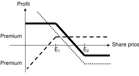
The profit pattern is shown in Figure 4 where the dotted and dashed lines represent the profit from the bought and sold put Options. The solid line symbolise the total profit from the strategy.

Figure 4. Bear Spread created with put Options. Source: (McMillan L. G., 1992).

If the share price (St) is less than E1 at the exercise date, the profit will be the difference

be-tween St-(E2+I). If the share price is between E1 and E2 at the exercise date, the profit is

equal to -(St - E1)-I. The strategy gives a negative profit if the share price is above E2 at the

exercise date.

2.3.3 Butterfly Spreads

Butterfly Spreads are suitable for investors with neutral prospects of the market, where large movement of the share price are unlikely to occur. The strategy involves the investor to take positions in Options with three different exercise prices. i.e. by buying a call Option with a relatively low exercise price, E1, and buying a call Option with a relatively high

exer-cise price, E3, and then selling two call Option with exercise price E2, between E1 and E3.

E2 are usually “at-the-money” (McMillan L. G., 1992).

The two dotted lines in Figure 5 represents the profit of the two purchased call Options and the dashed line represent the profit from the two sold call Options. The solid line symbolise the total profit form the strategy, indicating a profit if the share price is close to E2 but give rise to a small loss if the share price moves in any direction. Hence, the profit

equals to I if the St is below E1 or above E3 and to (St-E1)+(E3-St)-I if St is within E1 and E3

(with the assumption that E2 is in the exact middle of E1 and E3).

Profit

Share price Premium

Premium

Figure 5. Butterfly Spread created with call Options. Source: (McMillan L. G., 1992).

A Butterfly Spread can also be created with put Option and will than result in the same spread as when call Options are used.

2.3.4 Bottom Straddle

The following three strategies, sometimes called combinations, are created by taking posi-tions in both call and put Opposi-tions. Straddles and Strangles are the most popular ones, Straddles and Strangles are divided in two different types, bottom and top, where the top Straddle and top Strangle are the riskiest ones.

Investors who expect large movements on the market irrespective if the movements are positive or negative use Bottom Straddles. To create this strategy one buys call and put Op-tions with the same exercise price and exercise date. This causes high initial investments but in the same time gives the opportunity to yield high returns (Bailey R. E., 2005).

The profit pattern of a Bottom Straddle are shown in Figure 6 where the dotted lines illus-trates the profit from the long position of the call and put Option and where the bold line represent the total profit from the strategy.

Figure 6. Bottom Straddle created with call and put Options. Source: OMX Group.

One can observe that the profit possibilities are more or less unlimited but that it will only occur if the share price moves in any direction, one can also make out from figure 6 that

Profit Share price Premium Premium E1 E2 E3 Premium

Profit

Premium

Premium

E

Share price

the maximum loss will be equal to the initial investment. If St≤E the profit will be (E-St)-I

and if St>E the profit equals to (St-E)-I.

For investors who expect large movements on the market but think that it is more likely to for the share price to either increase or decrease there are two modified Straddles, called Strip and Strap, available. A Strip are created by buying one call Option and selling two put Options with the same exercise price and exercise date. The Strap is created in the opposite way.

2.3.5 Top Straddle

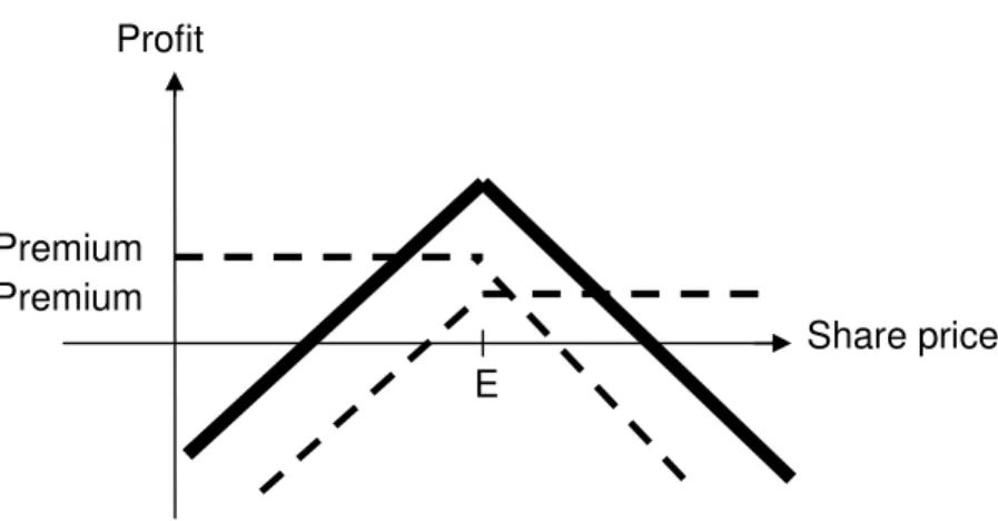
Top Straddle is the exact opposite of Bottom Straddle, created by selling call Options and buying put Options with the same exercise price and exercise date. The strategy is therefore suitable for investors who believe in a neutral future market and wants to gain profit from taking short positions (Hull J. C., 2006).

As shown in Figure 7 the Top Straddle is a highly risky strategy where the risk is unlimited if the share price moves in any direction at the expiration date and where the profit equals the premium from the short position if the share price is close to the exercise price.

Figure 7. Top Straddle created with call and put Options. Source: OMX Group.

2.3.6 Bottom Strangle

A Bottom Strangle is a similar strategy to a Bottom Straddle. The investor expects large movements on the market irrespective if the movements are positive or negative. It can be created by buying call Options with a high exercise price and buying a put Option with a low exercise price. Both Options should have the same exercise date. This causes higher initial investments than for a Bottom Straddle since the premium of a call Option and put Option increases when the exercise price is “in-the-money” compared to “at-the-money” (Bailey R. E., 2005). Profit Share price Premium Premium E

Figure 8. Bottom Strangle created with call and put Options. Source: OMX Group.

Figure 8 compared to Figure 6 indicate that the share price needs to move further for the investor to make a profit. The profit depends on how far apart the exercise prices are. If the share price at the exercise date are lower than E1 the profit equals to (E1-St)-I and if the

share price at the exercise date are higher than E2 the profit equals to (St-E2)-I. Profit will

be equal to the initial investment if the share price is between E1 and E2.

2.3.7 Top Strangle

A Top Strangle is a similar strategy to a Top Straddle but with the advantage of an accep-tance of larger movement of the share price. It is still a very risky strategy, which involves an unlimited potential loss, but it will yield a higher profit if it is successful because of a higher premium (Hull J. C., 2006).

Figure 9. Top Strangle created with call and put Options. Source: OMX Group.

As can be seen in figure 9 the profit from a Top Strangle is the opposite from a Bottom Strangle. As long as the share price stays within E1 and E2 a profit will yield. This strategy

can be appropriate for an investor who expects that large share price moves are unlikely and want to make profit from selling Options.

To sum up, the previous strategies are very useful for traders with different prospect and different risk preferences. Bull and Bear Spreads are for traders who have a positive or ne-gative prospect but prefer a smaller risk (cheaper premium) than they had been exposed of if they only bought call or put Options. For the reduction of the risk they have to give up

Profit Share price Premium Premium E1 E2 Premium Premium Profit Share price E 1 E2

some potential profit, they face a limit of profit that they would not have if they only bought call or put Options. Butterfly Spread is for traders with a neutral prospective, where the potential risk and profit are relatively small.

Bottom Straddle and Strangle suits investors who expect large movements on the market irrespective if the movements are positive or negative. A Bottom Straddle requires a higher initial investment than a Bottom Strangle but a Bottom Strangle requires larger movements of the underlying assets price to yield a profit than a Bottom Straddle. Top Straddle and Strangle is for investors with neutral prospects of the market, where large movement of the share price are unlikely to occur. The risk of these strategies are unlimited, the profit for a Top Straddle are higher than for a Top Strangle but a Top Straddle is at same time much more sensitive to price changes.

There are some downsides with these strategies even if they seem very attractive to use. For example if the general view of the market is that there will be a big change in a share price soon, the Option price will reflect that view and the investors will face an Option price that are significant more expensive than if the general view were otherwise. This relationship will affect the likelihood for one to receive profit from any given strategy and one should therefore only trade with Option when their own view differ from the general view5

.

3

Method

In 1973, Black, Scholes and Merton presented their epoch-making theory on how to price European call and put Options and since then brokers, investor and securities trader have used it. This chapter will go through how the Black-Scholes model for valuing European call and put Option is derived. It will also present some statistical definitions along with the method used in this thesis.

3.1

The Black-Scholes Formula

Black-Scholes pricing formula requires five variables, where three are directly observable: the current price of the underlying asset, the exercise price and the Options time to matur-ity. A fourth variable, the risk-free interest rate is needed to determine the present value of the exercise price. It is not directly observable but it is easily approximated by a treasury bond with the same time of maturity as the Option. Hence, one can call it effectively ob-servable. The only variable that is not observable is the underlying assets price volatility. Volatility is the standard deviation of the rate of change in the underlying asset price until the Option expires. It can obviously not be observed so investors use several techniques to estimate it (Black and Scholes, 1973).

The Black-Scholes formula for prices at time zero of an European call and put Option on a non-dividend paying share are:

) ( ) ( 1 2 0N d Ee N d S C = − −rT and P Ee N( d2) S0N( d1) rT − − − = − Where

C and P= Theoretical call and put price S0= Current share price

E= Exercise price

e= Natural logarithm (2.71828) r= risk-free interest rate T= Years to maturity

N(d)= Cumulative normal distribution function for a standardised normal distribution

T T r E S d σ σ /2) ( ) / ln( 0 2 1 + + = T d T T r E S d σ σ σ − = − + = ₁ 2 0 2 ) 2 / ( ) / ln(

σ

As can be seen from the Black-Scholes formula is that a high volatility (large price move-ments) results in a high Option price and a low volatility results in a low Option price.

3.2

Assumptions about Black-Scholes Formula

As most models, Black-Scholes pricing formula is based on a number of simplifying as-sumptions. If these assumption holds, the model should be adopted however this thesis will discuss and show how the model could be used even if some of the assumptions are fairly violated.

• Constant risk-free interest rate: Black-Scholes pricing formula assumes that the risk-free interest rate is known and constant through time. In reality there are no such thing as risk-free interest rate, therefore treasury bonds with the same time of maturity as the Option are used to represent it. Consequently, one could say that it is known although it is not constant over time. During periods of rapidly changing interest rates, rates are often subject to change, thereby violating this assumption. However, Merton (1973) constructed a model that allows one to relax this assump-tion. Due to simplicity reason that model will not be implied in this thesis even if the interest rate of the treasury bond might change.

• The share pays no dividends: A quite stringent assumption compared to the real world, studies with shares that have dividends will therefore have to make a neces-sary adjustment6

that needs to be done in order for the Black-Scholes model to still be applicable.

• Constant volatility: Black-Scholes pricing formula assumes that the volatility (standard deviation) of the rate of change in the underlying asset’s price is known and constant. Constant volatility or homoskedasticity is a very stringent assumption regarding financial data.

• European Option: Black-Scholes pricing formula assumes that the Option being priced is an European Option, that is, it can only be exercised at maturity. Euro-pean Option will therefore be used in this thesis analysis.

• No transaction cost: Black-Scholes pricing formula assumes that there are no transactions costs in buying or selling Options or the underlying asset. This is an assumption that will be used in this thesis because there is not enough reason to complicate the empirical part with any transactions costs, especially when the ef-fects are small.

• No penalties to short selling: A seller that does not own the underlying asset will simply accept the price of the asset from a buyer. Today this is a matter of course, everyone that takes a short position must leave a security margin except in the OTC.

3.3

Volatility

The main thread that runs through this thesis is about the volatility, particularly the need of having a conception of it. So let us try to break it down!

6 _{See Chance Don M. (1995) for adjustments of known dividends and Gemmill G. (1993) for adjustments of}

As mention in the introduction, there are four types of volatility: historical, implied, prog-nosticated and true (future). Historical volatility is simply how the price of an asset has moved relatively to the mean price throughout the history. The implied is referred to the volatility that is included within the Option price and the prognosticated is the volatility predicted by individuals. Future volatility is basically the true volatility, the actually move-ment of the assets price. The implied and the prognosticated volatility are the two more important volatilities, only if they differ one should trade with Options.

To estimate the volatility one studies the price of the underlying asset for a certain period. It can be derived from the following formula (Chance D. M., 1995):

1 ) ( 2 1 − − Σ = = = n u u Volatility i n i σ 3.3.1 Where

σ = The standard deviation of the underlying asset price i

u = The logarithmical price change from the previous observation

u= The average logarithmical percentage price change

n= Number of observations

It is difficult to decide an appropriate value for n. More data generally lead to more accu-racy if one believes the data to be stationary. Financial data are often far from stationary in first level, and as mention earlier in this thesis, constant volatility is therefore a too strin-gent assumption. Hence, if one acknowledges that σ does change over time and that too old data might not be relevant for predicting the future volatility, one would be forced to chose a value of n, themselves. Gemmill (1993) suggests that 110 observations ought to be used, whereas Chance (1995) suggests 60 observations. An often-used rule of thumb is to set n equal to the number of days of maturity of the Option, a rule that would not be pos-sible to use for Options with one or two years of maturity. The rule is therefore an indica-tion why traders might have to use more sophisticated methods when calculating the vola-tility.

3.4

Selection Process

As mentioned earlier in the introduction and in this chapter there is two variables, the vola-tility and the risk-free interest rate, that cannot be observed and has to be calculated for one to be able to use the Black Scholes formula. The three other variables can easily be ob-served. The data used to calculate the subsequent results are collected from Stockholms-börsen (OMX group) and from The Bank of Sweden and range from 2001 to 2002.

3.5

Calculate the Volatility

In order to calculate the volatility, irrespective if it is the historical or the true (future) the same technique from equation 3.3.1 has been used. However, one crucial difference has been made. When calculating the historical volatility one has to decide how many observa-tions that should be used (read about the trade off in chapter 3). This thesis follows Don M. Chance (1995) suggestion of 60 observations with the argument that too many observa-tions would not be relevant for any predicobserva-tions. To estimate the true (future) volatility, the

exact amount of observation, from the day that the Option was sold to the maturity day, has been used. In order to make the daily standard deviation (volatility) from equation 3.1 annualized, as Black Scholes formula requires, it has been multiplied by the square root of 250, which is the approximate number of trading days during a year. This has made both the historical and the true (future) volatility comparable with the implied volatility. The im-plied volatility is the standard deviation that constructs the theoretical price (the Black Scholes price) equal to the price the Option are bought and sold (the market price). The process of estimating the implied volatility is iterative and involves a trial-and-error search where different values are tested until the correct price is found.

3.6

The Risk-free Interest Rate

For the risk-free interest rate, one usually uses a treasury bond with the same time of ma-turity as the Option. This is because a treasury bond is the closes one can get to a risk free interest rate. One-month treasury bond with the same expiration date as the Option was chosen for the following computations, this was made to attain the best possible match. In order to make it continuously compounded, the natural logarithm of one plus the annual rate was taken.

3.7

Deviation

For analytical purposes, the following equations are used to measure biasness between true and implied volatility and between true and historical volatility:

Absolute deviation =

(

)

(

)

Mean of total sums of squares =

(

)

n T 2 σ σ − Σ 4.3 Where

σ = Either historical or implied volatility depend on what is presently compared T

σ = True volatility

Minimum, maximum and mean are calculated in the ordinary statistical way from the re-sults of the above equations. Since equation 4.3 gives more significance for large deviations than the mean calculated in equation 4.1 or 4.2 it will be the more decisive tool.

4

Result and Analysis

This part of the thesis will analyse Options with the OMX index as underlying asset. These Options are European, meaning that they can only be exercised on the maturity day, this makes it possible to use the Black Scholes formula. The OMX index is not an asset that one can buy or sell as it is, there is no perfect substitute either so the Option is therefore said to be naked, meaning that the holder is only obligated to pay the differential amount of money if it is exercised and not the index “assets” it self. Dividend is for the same reason excluded. Below one can see how the development of the OMX index.

Figure 10 shows how the OMX index, which is used as the underlying asset, fluctuated in year 2001 and in the beginning of 2002.

20₀₂ /02_/28 20₀₂ /02_/14 20₀₂ /01_/31 20₀₂ /01_/17 20₀₂ /01_/03 20₀₁ /12_/13 20₀₁ /11_/29 20₀₁ /11_/15 20₀₁ /11_/01 20₀₁ /10_/18 20₀₁ /10_/04 20₀₁ /09_/20 20₀₁ /09_/06 20₀₁ /08_/23 20₀₁ /08_/09 20₀₁ /07_/26 20₀₁ /07_/12 20₀₁ /06_/28 20₀₁ /06_/13 20₀₁ /05_/29 20₀₁ /05_/14 20₀₁ /04_/27 20₀₁ /04_/11 20₀₁ /03_/28 20₀₁ /03_/14 20₀₁ /02_/28 20₀₁ /02_/14 20₀₁ /01_/30 20₀₁ /01_/16 20₀₁ /01_/02 1150 1100 1050 1000 950 900 850 800 750 700 650 600

Figure 10. The OMX index price in year 2001, counted in SEK. Source: OMX Group.

Focus will be put on at-the-money call Options traded at Stockholmsbörsen in 2001, as the at-the-money put Option prices are very close to the call price the put Options will be as-sumed to show the same result.

In order to make the analysis as relevant as possible, a selection of Options is made based on the time to maturity. This is to reveal any differences in the biasness of the volatility be-tween Options with different maturity times.

Group 1: Maturity time is between 1 and 30 days Group 2: Maturity time is between 31 and 60 days Group 3: Maturity time is between 61 and 90 days

Figure 11 a-11 b are displayed for the interest of seeing how many Options of the call Op-tion in year 2001 that were exercised and gave a positive profit.

41,7% 58,3% Exercised Not Exercised Exercised Options 29,77% 70,23% Positive Profit Negative Profit Exercised Options with a positive profit

Figure 11 a-11 b. Percent of exercised Options and the percent of them with positive profit for the holder. Source: OMX Group.

Figure 11 a shows the percent of 729 at-the-money Options with the OMX index as under-lying asset that were and were not exercised. Whereas, Figure 11 b shows the percent of the exercised that gave the holder a positive profit. This analysis is not enough to draw any conclusions about the true volatility versus the implied and historical volatility but one can from this get an idea of what position that was more favourable in 2001. If one took a short position in an at-the-money call Option, one would almost have a 60 percent chance that it would not be exercised and one would get the profit equal to the Options premium. If one instead took a long position, one would only have around 12 percents (0.4*0.3) chance to have a positive profit.

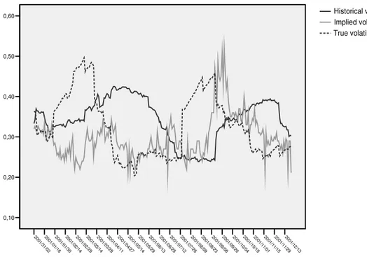
Considering Figure 13 underneath with the implied volatility from Options with maturity less than 30 days versus the true and historical volatility one can see that the implied and true volatility seems to move in at least the same way whereas the historical volatility moves in a less fluctuated way.

20₀₂ /01_/0 1 20₀₁ /12_/1 3 20₀₁ /11_/2 9 20₀₁ /11_/1 4 20₀₁ /10_/3 1 20₀₁ /10_/1 6 20₀₁ /10_/0 2 20₀₁ /09_/1 7 20₀₁ /09_/0 3 20₀₁ /08_/1 7 20₀₁ /08_/0 3 20₀₁ /07_/1 9 20₀₁ /07_/0 5 20₀₁ /06_/2 0 20₀₁ /06_/0 6 20₀₁ /05_/1 8 20₀₁ /05_/0 4 20₀₁ /04_/1 8 20₀₁ /04_/0 2 20₀₁ /03_/1 6 20₀₁ /03_/0 2 20₀₁ /02_/1 5 20₀₁ /02_/0 1 20₀₁ /01_/1 6 20₀₁ /01_/0 2 1,00 0,80 0,60 0,40 0,20 0,00 True volatility Implied volatility Historical volatility

Figure 13. The historical, implied and true volatility in comparison in year 2001 for Options in Group 1. Source: The author’s calculation based on data from OMX Group and Riksbanken.

The historical volatility estimate assumes that, the volatility that has prevailed in the recent past (this case the last 60 days) will continue in the future. As mentioned earlier this is a quite stringent assumption and this together with short time to maturity (less than 30 days) might cause this pattern.

From table 1, one can see that implied volatility deviates on average with a positive 3.35 percent, this means that the market price of at-the-money call Options in 2001 has been overvalued with 3.35 percent on average or in absolute terms with 0.0034.

Table 1 Deviations of implied and true volatility and of historical and true volatility for group 1. Source: OMX Group.

Group 1 N Minimum Maximum Mean

Deviation % Implied _{237 -76 % 108 % 3.35 %}

Deviation absolute Implied _{237 -0.36 0.25 0.0034}

Deviation % Historical _{237 -73 % 132 % -0.95 %}

Deviation absolute Historical _{237 -0.31 0.39 -0.0144}

Valid N (list wise) ₂₃₇

The implied volatility has been undervalued with 76 percent on its lowest moment and have been overvalued with 108 percent at it highest moment. Looking at the historical volatility, one will see an undervalued deviation of minus 0.95 percent. Hence, one can conclude that the historical volatility deviates less than the implied volatility on average for Options with a maturity time less than 30 days.

However, considering the mean of the total sums of squares in table 2, one will obtain a different conclusion where the implied volatility deviates less then the historical. This is be-cause table 2 is calculated by using equation 4.3 and therefore gives larger deviation more significant effect.

Table 2 Mean of total sums of squares of true and implied volatility and of true and historical volatility for group 1. Source: OMX Group.

Group 1 N Mean

Mean of total sums of squares of true andimplied volatility ₂₃₇

0.00635 Mean of total sums of squares of true andhistorical volatility _{237 0.00814}

Valid N (list wise) ₂₃₇

Looking at Figure 14, one will see that either the implied or the historical volatility for group 2 follows the true volatility in a faultless way. The implied volatility in February 2001 was around 0.25 whereas the true volatility was almost around 0.5, indicating that the mar-ket strongly undervalued the volatility at that time. At this time, it would have been better to buy volatility than to sell it i.e. to set up a Bottom Straddle.

20₀₁ /1 2/13 20₀₁ /1 1/29 20₀₁ /1 1/15 20₀₁ /1 1/01 20₀₁ /1 0/18 20₀₁ /1 0/04 20₀₁ /0 9/20 20₀₁ /0 9/06 20₀₁ /0 8/23 20₀₁ /0 8/09 20₀₁ /0 7/26 20₀₁ /0 7/12 20₀₁ /0 6/28 20₀₁ /0 6/13 20₀₁ /0 5/29 20₀₁ /0 5/14 20₀₁ /0 4/27 20₀₁ /0 4/11 20₀₁ /0 3/28 20₀₁ /0 3/14 20₀₁ /0 2/28 20₀₁ /0 2/14 20₀₁ /0 1/30 20₀₁ /0 1/16 20₀₁ /3 1/02 0,60 0,50 0,40 0,30 0,20 0,10 True volatility Implied volatility Historical volatility

Figure 14. The historical, implied and true volatility in comparison in year 2001 for Options in Group 2. Source: The author’s calculation based on data from OMX Group and Riksbanken.

Almost the opposite deviation occurred between the true and historical volatility in May 2001. This is stating that either the implied or the historical volatility would be trustfully in-dicators for Options with a maturity time between 31-60 days.

From Table 3, one can see that this picture is more or less confirmed. The deviation of the implied and the true volatility are on average 12.15 percent, this shows again that the mar-ket has overvalued the volatility.

Table 3 Deviations of implied and true volatility and of historical and true volatility for group 2. Source: OMX Group.

Group 2 N Minimum Maximum Mean

Deviation % Implied _{247 -31 % 117 % 12.15 %}

Deviation absolute Implied _{247 -0.15 0.26 0.0272}

Deviation % Historical _{247 -51 % 89 % -0.91 %}

Deviation absolute Historical _{247 -0.21 0.22 -0.0182}

Valid N (list wise) ₂₄₇

The highest overvalue was with 117 percent which could be seen as a very strong miscon-ception. Historical versus the true volatility is not much better than the implied when one consider the minimum and maximum deviations but if one looks at the average deviation, it is much better (-0.91 percent).

Looking at table 4 one will recognise a lower mean of the total sums of squares of the plied volatility then for the historical volatility. One could therefore conclude that the im-plied volatility is a better indicator of the true volatility then the historical volatility, at least on average when it comes to Options within the maturity group 2.

Table 4 Mean of total sums of squares of true and implied volatility and of true and historical volatility for group 2. Source: OMX Group.

Group 2 N Mean

Mean of total sums of squares of true andimplied volatility ₂₃₇

0.00607 Mean of total sums of squares of true andhistorical volatility _{237 0.00720}

20₀₁ /1 2/1₇ 20₀₁ /1 2/0₃ 20₀₁ /1 1/1₉ 20₀₁ /1 1/0₅ 20₀₁ /1 0/2₂ 20₀₁ /1 0/0₈ 20₀₁ /0 9/2₄ 20₀₁ /0 9/1₁ 20₀₁ /0 8/2₈ 20₀₁ /0 8/1₄ 20₀₁ /0 7/3₁ 20₀₁ /0 7/1₇ 20₀₁ /0 7/0₃ 20₀₁ /0 6/1₈ 20₀₁ /0 6/0₁ 20₀₁ /0 5/1₇ 20₀₁ /0 5/0₃ 20₀₁ /0 4/1₈ 20₀₁ /0 4/0₂ 20₀₁ /0 3/1₉ 20₀₁ /0 3/0₅ 20₀₁ /0 2/1₉ 20₀₁ /0 2/0₅ 20₀₁ /0 1/1₉ 20₀₁ /0 1/0₅ 0,60 0,50 0,40 0,30 0,20 0,10 True volatility Implied volatility Historical volatility

Figure 15. The historical, implied and true volatility in comparison in year 2001 for Options in Group 3. Source: The author’s calculation based on data from OMX Group and Riksbanken.

Considering Figure 15, one can observe that it almost looks like figure 14. Thus, neither the historical nor the implied volatility for group 3 follows the true volatility in a faultless way. An interesting observation is that the historical and the true volatility seem to have an al-most perfect negative correlation.

One can also observe that from September to December the implied volatility has generally overvalued the true volatility, which indicates that selling strategies i.e. a Top Straddle wo-uld have been preferable to use.

Table 5 confirms the above observation of group 3’s pattern of the historical and true vola-tility. Hence, there is a low average deviation of -0.16 percent while the maximum and minimum deviations are large, -0.43 percent and 0.68 percent respectively. Which are both signs of negative correlation.

Table 5 Deviations of implied and true volatility and of historical and true volatility for group 3. Source: OMX Group.

Group 3 N Minimum Maximum Mean

Deviation % Implied _{245 -35 % 112 % 18.17 %}

Deviation absolute Implied _{245 -0.13 0.24 0.0402}

Deviation % Historical _{245 -43 % 68 % -0.16 %}

Deviation absolute Historical _{245 -0.18 0.17 -0.0163}

From Table 5 one can see that implied volatility is once again overvalued, this time with 18,17 percent on average. The minimum deviation for the implied volatility is less than the minimum deviation for the historical volatility. However, it is the opposite for the maxi-mum deviation, 112 percent and 68 percent.

Table 6 Mean of total sums of squares of true and implied volatility and of true and historical volatility for group 3. Source: OMX Group.

Group 3 N Mean

Mean of total sums of squares of true andimplied volatility ₂₃₇

0.00622

Mean of total sums of squares of true andhistorical volatility _{237 0.00684}

Valid N (list wise) ₂₃₇

The historical volatility does not only show signs of a negative correlation, it also has a higher mean of total sums of squares. Hence, implied volatility seems to be a better indica-tor for the true volatility than the hisindica-torical volatility when the maturity time is between 61 and 90 days.

A short summery of this chapter shows that neither the historical nor the implied volatility has been a perfectly good indicator for the true volatility in 2001, regardless time to matur-ity. The historical volatility deviates less as longer the time to maturity is. For group 1 the mean of total sums of squares was 0.00814 for group 2 it was 0.0072 and for group 3 it was as low as 0.0068. This could indicate that the historical volatility is better to predict the true volatility for Options with more extended maturity time. The implied volatility does not show any similar pattern when it comes to different maturity times.

However, the tables of the mean of total sums of squares show an overall lower mean for the implied volatility than the historical volatility. Thus, the implied volatility seems to gives an on average better prediction of the true volatility than the historical volatility, regardless of time to maturity.

5

Conclusions and Further Research

The purpose of this thesis was to investigate if one can learn anything from the history of the volatility. Is the historical volatility when using Black-Scholes assumption of constant volatility better to predict the true (future) volatility than the implied volatility? Can anyone make profit with a different conception of the future volatility?

The main conclusion that can be drawn from this study of Options on the OMX index in year 2001 is that the implied volatility seems to be better to predict the true volatility than the historical volatility. Neither one of them is perfect indicators of the true volatility but the implied volatility deviates less from the true volatility than the historical volatility on av-erage.

From the selection made of the Option with different maturity times one can conclude that the implied volatility is better to predict the true volatility for Options with short time to maturity. From the same selection, one can conclude that opposite condition exist for the historical volatility, even though it is not as low as it is for the implied volatility. Remem-bering what Black and Scholes establish from their study in 1972, that using past data to es-timate the volatility caused the formula to overvalue the Options on high volatility assets and undervalue Options on low volatility assets, one can imagine what variety of effects of Options volatility that could occur with different maturity times. This thesis result is there-fore supporting Black and Scholes conclusions.

First, when one compares the true volatility with the implied volatility one will be able to say if a profit would have been made with a different conception of the future volatility. The maximum deviation between the implied and true volatility were measured to 117 per-cent, this means that the market undervalued the volatility with 117 percent. If a person had had another conception and thought that the market had undervalued the volatility and set up a Bottom Straddle or Bottom Strangle that person would have made a significant profit. The same opportunity of making a major profit could have occurred when the mar-ket strongly overvalued the volatility buy 76 percent but in that case, one would have to create a Top Straddle or a Top Strangle.

To conclude the history of the volatility one can establish the fact that the volatility that re-flects in Option prices does not very often correspond with the true volatility. No one have the power or the insight to prognosticate the future volatility perfectly incessantly. Yet, it is the differences in people’s conceptions of the volatility that create the trade with Option and makes it to such an interesting and useful tool.

A suggestion to further studies would be to make a similar study, but more extensive i.e. using five or six different Options and for a longer period with the purpose of drawing more general conclusions about Options. In addition, one could try to make a more so-phisticated model to calculate the future volatility by using historical data i.e. ARCH- or a GARCH-model, to investigate if those models would diverge more from the implied and the true volatility.

Another suggestion would be to analyse Options outcome, concerning the profit, and in-vestigate if there could be any advantages in taking a certain position. However, to do that one would again need to make an extensive analysis covering at least 10 different Options for a period of 5-10 years.

References

Bailey R. E. (2005) The Economics of Financial Markets, Cambridge University Press, UK

Björk Tomas (1998) Arbitrage Theory in Continuous Time, Oxford University Press inc., New York

Black F. and Scholes M. (1972) “The Valuation of Option Contracts and a Test of Market Efficiency”, Jour-nal of Finance, Vol. 27, May 1972, pp 399-418.

Black F. and Scholes M. (1973) “The Pricing of Options and Corporate liabilities”, Journal of Political Econ-omy, Vol. 81, May/Jun 1973, pp 637-659.

Chance Don M. (1995) An Introduction to Derivatives, 3rd _{edition, The Dryden Press, USA.}

Engle R. (1982) Autoregressive Conditional Heteroscedasticity with Estimates of the Variance of UK Inflation, Economet-rica, 50 (1982), pp 987-1008.

Enders W. (2004) Applied Econometric Time Series, 2nd _{edition, John & Sons Inc, USA}

Fischer, Black and Scholes (1971) “The Pricing of Options and Corporate Liabilities”, The Journal of Political Economy, USA.

Galai Dan (1977) “Tests of Market Efficiency of the Chicago Board Options Exchange”, Journal of Business, Vol. 50, April 1977, pp 167-97.

Gemmill G. (1993) Options Pricing – An International Perspective, McGraw-Hill Book Company, London. Gustaf Hagerud (2002) ”En introduktion om den Svenska finansmarknaden”, SERO, Dreamstone AB,

Stockholm.

Hull John C. (2003) Options Futures and Other Derivatives, 5th _{edition, Princeton Hall, Upper Saddle River, New}

Jersey, USA.

McMillan L. G. (1992) Options as a Strategic Investment, New York Institute of Finance, New York

Merton R (1973) “Theory of Rational Option Pricing”, Bell Journal of Economics and Management Science, Vol. 4, No 1, 1973, pp 141-183.

Ross, Westerfield and Jaffe (2005) Corporate Finance, McGraw-Hill Book Company, New York.

Sandås Patrik (1991) “Pricing of European Bond Options: A Nonparametric test of the Ho-Lee Model”, Working Paper from SHH

Stockholmsbörsen (2003) ”Option – En tidning om dina valmöjligheter på Stockholmsbörsen”, nummer 2, Strokirk Landströms, Stockholm.

Internet References http://www.finansportalen.se/utbildningoptioner.htm, Feb 2006 http://www.se.omxgroup.com, Feb 2006 http://www.se.omxgroup.com/se/publikationer/pdf/Option%201.02_webb.pdf , Mars 2006 http://domino.omgroup.com/www/WebTransaction.nsf/attachments/strategiermedoptioner/$file/Strategi er_for_varje_marknad.pdf, Mars 2006